Cow-Calf Farm Management: Farm survey evidence from
2007
Richard F. Nehring, Derrell Peel, and David Nulph
Prepared for the
Southern Association of Agricultural Economists
2009 Annual Conference
January 31-February3, 2009
Atlanta, Georgia
Key Words:
Cow-calf, performance measures, technical efficiency
January 14, 2009
Richard Nehring is an agricultural economist with the Resource and Rural Economics Division, Economic Research Service, Derrell Peel an agricultural economist at Oklahoma State University, and David Nulph is a geographic information analyst with the Information Services Division
E-mail: rnehring@ers.usda.gov
Postal address: ERS, 1800 M Street NW, Washington, D.C. 20036-5831. The views expressed are the authors’ and do not necessarily represent policies or views of the U.S. Department of Agriculture.
Abstract
This study describes and compares cow-calf operations and assesses their relative competitiveness, developing performance measures for a sample of U.S. farms. We find that larger operations tend to be significantly more scale and technically efficient than smaller
operations. However, we do not find significant differences in net farm returns by size except on medium large operations—showing virtually no net return on farm assets in 2007. While larger operations are clearly more scale and technically efficient and have lower variable costs per cow, off-farm income makes smaller operations competitive as reflected in higher household returns than all size groups--except for very large cow-calf operations.
Background:
Beef cow-calf operations vary considerably in size, available resources, profitability, and the use of technology. Opportunities remain to improve management practices, both production and financial, in many cow-calf operations in major cow-calf states (Beef Cattle Manuel). Beef cattle industry analyst Bill Helming recently outlined eight important trends occurring in the U.S. beef cattle industry that either directly or indirectly affect cow-calf operations: 1) consolidation accelerating due to excess capacity, 2) more direct cattle ownership in feedlots and less custom feeding, 3) cattle placement weights increasing due to high energy prices, 4) feedlot
backgrounding (i.e. providing high energy rations to bigger calves on cow-calf sites in
preparation for shipping at higher weights to feedlots) opportunities on cost-competitive feedlot operations given higher placement weights, 5) feedlot locations moving toward corn production locations, thus putting a greater premium on cutting transportation costs, 6) less flaked corn at the feedlot level and more dry corn and byproducts given high energy prices, 7) increasing domestic and export demand for beef, and 8) brand opportunities with feeding operations and beef packing companies partnering (Feedstuffs November 3, 2008).
In this study, we focus on the consolidation issue using stochastic production frontier (SPF) procedures to estimate the impact of size and off-farm income on competitiveness. We
hypothesize that increasing size and off-farm income from both the operator and the spouse enhance competitiveness.
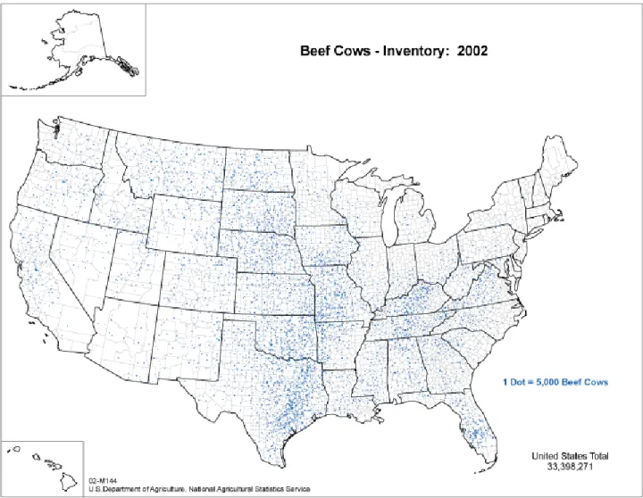
Beef cow-calf production is relatively widespread and economically important in the United States. Figure 1 identifies the number of beef cows in important Agricultural Statistics Districts (ASDs) and Figure 2 characterizes the relative importance of these ASDs in cow-calf production. According to the 2002 Census of Agriculture, close to 800,000 farms held more than 33 million beef cows (Figure 3). Beef cow inventories1 are steady compared to 1997 while farm numbers dropped by about 100,000, suggesting consolidation trends.
Cow-calf operations are located throughout the United States, typically on land not suited or needed for crop production ( http://www.ers.usda.gov/briefing/cattle/Background.htm; Peel). In Figure 4 we see close to half of cow-calf operations are located in ASDs with farms averaging more than 500 acres of pasture. These operations are dependent upon range and pasture forage conditions, which are in turn affected by variations in the average level of rainfall and
temperature for the area. Beef cows harvest forage from grasslands to maintain themselves and raise a calf with little, or no grain input, and are generally on lower priced land as shown in Figure 5. The cow is maintained on pasture year round, as is the calf until it is weaned. If
additional forage is available at weaning, some calves may be retained for additional grazing and growth until the following spring when they are sold. The average beef cow herd is about 50 head, but operations with 100 or more beef cows comprise more than 9 percent of all beef operations (the same as 1997) and 61 percent of the beef cow inventory, compared to 49 percent in 1997. Operations with 50 or fewer head are largely part of multi-enterprises, or are
supplemental to off-farm employment—i.e. hobby farms (USDA/ERS 2001).
Objectives: This study will: 1) identify the important economic and technical characteristics of cow-calf operations by region—Corn Belt, Northern Plains, Appalachia, Southeast, Delta,
Southern Plains, Mountain, and Pacific for the 22 leading cow-calf states (footnote 1), 2) identify characteristics by size—0 to 120 cows2, 121 cows to 300 cows, 301 cows to 500 cows, 501 cows to 1,000 cows and greater than 1000 cows; and 3) calculate farm-level economic performance measures and assess factors influencing scale and technical efficiency in on operations with more than 30 beef cows using a stochastic production frontier approach.
Data Sources and Methods: This analysis is based on information from the recently released 2007 ARMS phase III survey, which collects information on the number of beef cows per farm and on costs and returns on these operations3. The ARMS data source allows a comparison of costs and returns by size and by region. The 2007 ARMS survey contains 3,915 observations on farms that report beef cows. We will also use recently developed regression techniques that allow us to relate several outputs to several inputs in a single equation to develop measures of technical (best practice production techniques) and scale efficiency scores by farm.
Table 1 presents information on cow-calf production by region in the 22 states analyzed. The western regions--Mountain, Pacific, and Southern Plains--account for close to one-third of cow-calf value of production, based on 2007 ARMS survey data, and along with the Northern Plains and Corn Belt dominant cow-calf production.
and commercial operations account for more than 21 percent http://www.aphis.usda.gov/vs/ceah/ncahs/nahms/. In this study we do not differentiate between these operations and commercial cow-calf operations.
2 Size groupings used in the tables were chosen to correspond to actual beef cows—including beef heifers that had calved----per farm and are arbitrary groupings. The SPF estimation also includes all other beef animals on the beef cow farm, and all other livestock on the farm. For example, in Table 2 the group with 30 to 120 beef cows, as defined above, averages 55.5 beef cows, 86.5 beef animals (including beef cows), 9.8 hogs, 0.9 dairy, and 1,744 poultry per farm.
3 States and their designated regions included in this dataset include: NORTHERN PLAINS: KS, NE, ND, SD; DELTA: AR, LA; CORN BELT: IA, MO; APPALACHIA: KY, TN, VA; SOUTHEAST: AL, FL, GA; SOUTHERN PLAINS: OK,TX; MOUNTAIN WEST: AZ, CO, NM, WY; and PACIFIC: CA, OR. These 22 states will be included in the 2008 ARMS Cost of Production Survey.
The comparison of summary data at the regional level shown in Table 1 and Figure 3 indicates that stocking rates (potential pasture acres per cow) are substantially higher and variable costs per cow are significantly lower in the three western regions---compared to the remaining regions. Table 1 also shows that relatively little corn production occurs on cow-calf operations in the western regions, on average. These observations suggest different production technologies in the Western regions compared to the eastern regions. However, to give an overview of the competitiveness by size group in the cow-calf industry, our econometric estimates of performance measures will include all regions. Finally, we chose to focus on cow-calf operations with greater than 30 cows. This allows us to capture performance issues in commercial operations while still including smaller operations that rely on off-farm income (see Figures 6 through 8 identifying the pervasiveness of off-farm income, particularly in the
Southern regions) in addition to sales from cow-calf operations—thus recognizing the bimodal nature of the cow-calf industry from the Census of Agriculture data.
We use stochastic production frontier (SPF) measurement to econometrically estimate the input distance function DI(X,Y,R) where X refers to a vector of inputs, Y refers to a vector of outputs, and R refers to a vector of environmental or shift factors, such as soil texture and size groupings. Approximating this function by a translog functional form to limit a priori restrictions on the relationships among its arguments results in: where i denotes farm, t time period, k,l, outputs, m,n, inputs, and q,r the technical/environmental (including for example age or rented land) variables.
This functional relationship, which embodies a full set of interactions among the X, Y and R arguments of the distance function, can be more compactly written as -ln X 1,it = TL(X/X1,Y,t) =
TL(X*,Y,t)4. We append a symmetric error term, v to equation (1) to account for noise, and also change the notation “- ln Dit” to “u”. The resulting -ln X1 = TL(X*,Y,R) + v - u function (with
the sub-scripts suppressed for notational simplicity) may be estimated by maximum likelihood (ML) methods, to impute the TE measures as the distance from the frontier. For the SPF model
-u thus represents inefficiency; the efficiency scores generated by FRONTIER5 essentially measure exp(-U) = DI(X*,Y,R). This is therefore our measure of technical efficiency.
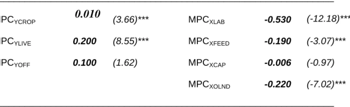
A parametric input distance function approach is used to estimate performance measures, including RTS (returns to scale) and TE (technical efficiency). The input distance function is denoted as DI(X,Y,R), where X refers to inputs, Y to outputs, and R to other farm efficiency determinants. For the analyses, three outputs developed from the ARMS data for cow-calf farms are: YCROP = value of crop production, YLIVE = value of livestock production, and YOFF = off-farm
income. Inputs are: XLAB = labor, XCAP = capital, XFEED = feed and miscellaneous including
fertilizer and fuel, and XOLND = land.
Estimating DI(X,Y,R) requires imposing linear homogeneity in input levels (Färe and Primont), which is accomplished through normalization (Lovell et al.); DI(X,Y, R)/X1 = DI(X/X1,Y, R) =
DI(X*,Y, R). Approximating this function by a translog functional form to limit a priori restrictions on the relationships among its arguments results in:
(2a) ln DIit/X1,it = α0 + Σmαm ln X*mit + .5 ΣmΣnαmn ln X*mit ln X*nit + Σkβk ln Ykit
+ .5 ΣkΣlβkl ln Ykit ln Ylit + ΣqφqRqit + .5 ΣqΣrφqrRqitRrit + ΣkΣmγkm ln Ykit ln X*mit
+ ΣqΣmγqm ln Rqit ln X*mit + ΣkΣqγkq ln Ykit ln Rqit + vit = TL(X*,Y, R) + vit, or
(2b) -ln X1,it= TL(X*,Y, R) + vit - ln D I
it = TL(X*,Y, R) + vit - uit,
4 By definition, linear homogeneity implies that DI(ωX,Y,R) = ωDI(X,Y, R) for any ω>0; so if ω is set arbitrarily at 1/X1, DI(X,Y, R)/X1 = DI(X/X1,Y, R).
5 We used Tim Coelli’s FRONTIER package for the SPF estimation, and computed the measures and t-statistics for measures using PC-TSP.
where i denotes farm; t the time period; k,l the outputs; m,n the inputs; and q,r the R variables. We specify XOLND as land, so the function is specified on a per-acre basis, consistent with much
of the literature on farm production in terms of yields.
The distance from the frontier, -ln DIitis explicitly characterized as the technical inefficiency error-uit. As in Battese and Coelli,we use maximum likelihood (ML) methods to
estimate (2b) as an error components model. The one-sided error term uit is a nonnegative
random variable independently distributed with truncation at zero of the N(mit,σu 2
) distribution,
wheremit=Ritδ, Ritis a vector of farm efficiency determinants (assumed here to be the factors in
the R vector), and δ is a vector of estimable parameters. The random error componentvitis assumed to be independently and identically distributed, N(0,σv
2). More precisely, we estimate a household model with three outputs, crops, livestock, and off-farm income, (measured as earned income relating to wages, agricultural and other rents, and earnings from another business— passive income such as pensions and social security, interest income etc is not included), and four inputs—labor, miscellaneous expenses, capital, and land.
This function is estimated using SPF techniques. Technical efficiency is characterized assuming a radial contraction of inputs to the frontier (constant input composition). The econometric model includes two error terms to represent the distance from the frontier: a random (white noise) error term,vit, assumed to be normally distributed, and a one-sided error
term, uit, assumed to be distributed as a half normal.
The productivity impacts (marginal productive contributions, MPC) of outputs or inputs can be estimated from this model by the first order elasticities, MPCm = -εDI,Ym = -∂ln D
I
(X,Y,R)/∂ln
Ym = εX1,Ym and MPCk = -εDI,X*m = -∂ln D I
(X,Y,R)/∂ln X*k = εX1,X*k. MPCm indicates the increase in overall input use when output expands (and so should be positive, like a marginal cost or output
elasticity measure), and MPCk indicates the shadow value (Färe and Primont) of the kth input
relative to X1 (and so should be negative, like the slope of an isoquant). Similarly, the marginal
productive contributions of structural factors, including soil texture (TEXT), water holding capacity (WATHCA), and urban influences as measured by Nehring et al. (Popacc), can be measured through the elasticities, MPCRq = -εDI,Rq = -∂ln D
I
(X,Y,R)/∂Rq = εX1,Rq . If εX1,Rq <0, an increased Rq implies that less input is required to produce a given output, which implies
enhanced productivity, and vice versa.7
Scale economies (SE) are calculated as the combined contribution of the M outputs Ym, or
the scale elasticity SE = -εDI,Y = -Σm∂ln D I
(X,Y,R)/∂ln Ym = εX1,Y. That is, the sum of the input
elasticities, ∑m∂ln X1/∂ln Ym, indicates the overall input-output relationship and thus returns to
scale. The extent of scale economies is thus implied by the short-fall of SE from 1; if SE<1, inputs do not increase proportionately with output levels, implying increasing returns to scale. Finally, technical efficiency (TE) “scores” are estimated as TE = exp(-uit.). The impact of
changes in Rq on technical efficiency can also be measured by the corresponding
δcoefficient in the inefficiency specification for -uit.
It is assumed that the inefficiency effects are independently distributed, and uit arise
by truncation (at zero) of the normal distribution with meanμit, and variance σ 2
, where the
mean ofμitis defined by
(3) μit= δ0 + δ1 (Popaccit) +δ2 ln (OPLABORit) + δ3ln (SPLABORit) + δ4ln (TOTAUit)
In equation (3), variables are measured as follows: Popaccit , is an index measured as the
operator hours worked off farm, SPLABORit represents hours of spouse hours worked off
farm, and TOTAU measures the total number of animal units on the farm. Theδ1
-parameter, measuring the effect of urbanization on the inefficiency model in equation (3), is expected to have a negative effect on the size of the inefficiency effects. That is, higher urbanization is negatively related to technical efficiency. The sign on theδ2 –parameter, theδ3 –parameter, and theδ4 –parameter, measuring the impacts of labor and total animal units, is less clear. Evidence in Fernandez et al. suggests that operator hours worked off farm are negatively related to technical efficiency—the argument being that off-farm work by the operator in particular is inimical to best practice farming on managerially intensive dairy operations. Evidence in Kompas relating to dairy farms suggests that total animal units are positively related to technical efficiency.
Stochastic Frontier Results
More than one-half of the estimated coefficients from the input distance function are significant as shown in Table 3, including the own price on labor, and the own cross price effects for crops, livestock, and off-farm income. All of the measures of outputs and inputs have the expected signs, positive for outputs and negative for inputs, as shown in Table 4. All are significant or marginally significant except for capital. Among the inefficiency effects, we find that operator off-farm hours are positively associated with higher technical efficiency—spouse off-farm hours are only marginally significant, but tend to suggest the notion that spouse hours off-farm also boost technical efficiency. And, we also find that operations with more animal units (including all species) are more technically efficient than operations with smaller livestock populations.
Conclusions
We find that larger operations tend to be significantly more scale and technically efficient than smaller operations. However, we do not find significant differences in net farm returns by size except on medium large operations—which showed virtually no net return on farm assets in 2007. While larger operations are clearly more scale and technically efficient and have lower variable costs per cow, off-farm income makes smaller operations competitive as reflected in higher household returns than all size groups except for very large cow-calf operations. In future research the availability of more detailed cost of production information will facilitate identifying competitiveness by region and size.
References
Beef Cattle Manuel, “Chapter 1. Beef Industry Overview for Oklahoma,” Damona Doye and David Lalman, Oklahoma State University, Stillwater, Oklahoma, 2004.
Battese, G. E., and T. J. Coelli. "A Model for Technical Inefficiency Effects in a Stochastic Frontier Production Function for Panel Data." Empirical Economics 20(1995):325-332. Coelli, T. "A Guide to FRONTIER Version 4.1: A Computer Program for Stochastic Frontier Production and Cost Function Estimation." mimeo, Department of Econometrics, University of New England, Armidale, 1996.
Coelli, T., and G. Battese. "Identification of Factors Which Influence the Technical Inefficiency of Indian Farmers." Australian Journal of Agricultural Economics 40(1996):103-28.
Dubman, R.W. Variance Estimation with USDA’s Farm Costs and Returns Surveys and Agricultural Resource Management Study Surveys. Washington DC: U.S. Department of Agriculture, Economic Research Service Staff Paper AGES 00-01, 2000.
Farell, M.J., The Measurement of Productive Efficiency, Journal of the Royal Statistical Society, series A, General, 120 (3). 1957.
Färe, R., and D. Primont. 1995. Multi-Output Production and Duality: Theory and Applications. Kluwer Academic Publishers: Boston.
Feedstuffs, “Cattle market outlook shows some promise,” Minnetonka, Minnesota, November 3, 2008.
Fernandez, Jorge, Richard F. Nehring, and Ken Erickson, “Off-farm Work and Economic Performance of Crop and Livestock Farms.” Paper presented at the annual meetings of SAEA in Mobile, Alabama, February, 2007
Kompas, Tom., and Tuong Nhu Che. “Technology Choice and Efficiency on Australian Dairy Farms.” Journal of Agricultural and Resource Economics 50,1(2006): 65-83.
Lovell, C.A.K., S. Richardson, P. Travers and L.L. Wood. 1994. “Resources and Functionings: A New View of Inequality in Australia”, in Models and Measurement of Welfare
and Inequality,(W. Eichhorn, ed.), Berlin: Springer-Verlag Press.
Morrison-Paul, Catherine, Richard Nehring, David Banker and Agapi Somwaru. “Are Traditional Farms History?” Journal of Productivity Analysis, 22 (2004): 185-205.
Nehring, R., C. Barnard, D. Banker and V. Breneman, “Urban Influence on Costs of Production in the Corn Belt,” American Journal of Agricultural Economics 88, 4 (2006): 930-946.
Comparison of Intensive and Pasture-Based Systems,” Paper presented at the annual SAEA meetings in Mobile, Alabama, February 4-7, 2007.
Peel, Darrell S, “Beef Cattle Growing and Backgrounding Programs,” Vet Clin Food Anim Pracs 19 (2003): 365-385.
U.S. Department of Agriculture, Economic Research Service (USDA/ERS). Characteristics and Production Costs of U.S. Cow-Calf Operations. Statistical Bulletin Number 974-3, Washington DC, November, 2001.
U.S. Department of Agriculture, Economic Research Service (USDA/ERS). Agricultural Resource Management Survey, Phase III 2007. Washington DC, 2008.
U.S. Department of Agriculture, Economic Research Service (USDA/ERS). Briefing room.
http://www.ers.usda.gov/briefing/cattle/Background.htm. Washington DC, 2008.
U.S. Department of Agriculture, Economic Research Service (USDA/NASS). U.S. Census of Agriculture, 1997 and 2002. Washington DC.
USDA, APHIS, Part III: Reference of 1997 Beef Cow-Calf Production Management and Disease Control, National Animal Health Monitoring System, January 1998.
Table1. Cost and Production Means and Statistics by Region all observations in the 22 most important cow-calf states, 2007
Item Corn Belt
Northern Plains
Appalachia Southeast Delta
Southern Plains Mountain
Pacific Number of Observations 654 931 262 657 390 709 162 150 Percent of farms 14.0 12.4 15.7 10.4 6.7 31.4 5.0 4.2 Percent of value of production 2 17.2 27.7 7.1 9.7 7.9 17.0 9.1 4.4 Percent of pasture acres 2 4.3 16.8 2.9 3.2 2.1 35.0 31.0 4.8 Percent of corn acres 2 33.3 49.2 5.1 1.7 0.5 7.1 3.0 1.0 Percent of hay acres 2 13.7 30.4 12.4 3.5 4.6 21.1 11.1 3.1
Beef Cows per Farm
45.1 BCGH 91.1 ACDEFGH 27.8ABDEFGH 40.2BCFGH 43.4BCGH 50.5BCDG 111.9ABCDEFHI 61.2ABCDG Net Return on
Assets Farm (%)
2.7 JBDEF 4.8 ACDEFH 1.8BDEF 0.7ABCG 0.4ABCG 0.5 2.7 DEF 1.7B
Net Return on Assets All In (%)
6.2 DH 7.7 DH 8.3DH 4.7ABCEF 7.4DH 8.1DH 5.4 4.4ABCEF
Variable Cost per Cow $
1,343BCFGH 1,077ACDEFGH 1,159AFGH 1,345FBFGH 1,411BFGH 768ABCDE 663ABCDE 775ABCDE
Land price ($/acre) 2,484 BCDFG 861 ACDEFH 3,354 ABEFGH 4,102 ABEFGH 2,233 BCDEFG 1,194 ABCDEGH 696 ACDEFH 2,053 BCDFG
Off-farm income/ total Income (%)
26.8BCDEF 15.6ACDEFH 55.7ABCDGH 38.8ABCFG 50.1ABGH 52.6ABCDGH 26.4CDEF 31.8BCEF
Contracts/total production (%)
21.5CDE 16.7CDE 49.2ABEF 60.3CDE 76.0ABCDFGH 14.0CDE 28.0DE 39.3E
Operator hrs off-farm
493CEF 538CF 836ABGH 658G 690AG 805 ABGH 363CDEF 587CF
Spouse hours off-farm 467B 617ACEFH 436B 428 399B 488B 753H 317B FORAGE INTENSITY Potential pasture acres/cow
2.60BDFGH 4.91ACDEFG 2.99BDEFGH 3.304ABCFGH 2.95BCFGH 8.14 ABCDEG 21.53ABCDEFH 7.23ACDEG
Purchased feed/ total costs
18.5DEH 20.2DEH 21.4DEH 35.3ABCEF 53.0ABCDFGH 19.3DEH 31.2E 36.0ABCEF
Hay yield (tons/ac) 2.35CH 2.05EFH 1.86ADEFH 2.57C 2.46BCH 2.59BC 2.17H 3.44ABCEG
______________________________________________________________________________________________________________________________________ _
= Appalachia, D = Southeast, E = Delta, F = Southern Plains, G = Mountain, H =Pacific.
Table 2. Economic performance by size groupings, 2007
Item 30 to 120 Beef Cows 121 to 300 Beef Cows 301 to 500 Beef Cows 501 to 1000 Beef Cows Greater than 1000 Beef Cows Number of Observations 1,059 996 313 145 99 Percent of farms 66.0 26.9 4.8 1.3 0.9 Percent of value of production 2 31.7 33.9 12.3 5.6 16.6
Percent of pasture acres 2 22.5 28.2 19.9 12.2 17.3
Percent of corn acres 2 40.0 39.6 10.7 4.2 5.5
Percent of hay acres 2 39.0 38.8 9.6 5.3 7.2
Beef Cows per Farm 55.5 BCDE 154.3ACDE 325.4ABDE 592.6ABCE 1425.1ABCD
Net Return on Assets Farm (%)
2.3 2.5D 2.4 0.8B 5.1
Net Return on Assets All In (%)
7.9BCD 4.8A 4.2A 2.5A 6.9
Returns to Scale 0.284BCDE 0.344ADE 0.376AE 0.410AB 0.422ABC
Efficiency score 0.765D 0.783E 0.791A 0.803 0.811AB
Variable Cost per Cow $ 1,094BCDE 801ACD 592AB 552AB 652A
Land price ($/acre) 1,839 BCDE 1,244ACDE 795AB 619AB 651AB
Off-farm income/ total Income (%)
44.3BCDE 19.0ACE 11.4ABE 10.8AE 0.9ABCD
Contracts/total production (%)
32.2BD 24.5AD 24.2D 3.5ABCE 35.9D
Operator hrs off-farm 653BCE 416ACE 211AB 394 107AB
Spouse hours off-farm 541 540 372A 366 L
FORAGE INTENSITY Potential pasture acres/cow 5.91C 6.23C 9.27AB 10.76 6.88 Purchased feed/ total costs 22.1CE 25.9E 32.7AE 27.2E 54.6ABCD
Wheat yield (bu/ac) 30.00B 33.86AC 24.97BE 30.00 36.32C
____________________________________________________________________________________________________________________________________________ _
Source: Authors’ analysis of USDA Agricultural Resource Management Survey USDA (2007). a. The t-statistics are based on 2,582 observations using weighting techniques described in Dubman. A through J indicate significant differences in means across columns with A = cow-calf operations with 30 to 120 cows, B = cow-calf operations with 121 to 300 cows, C = cow-calf operations with 301 to 500 cows, D = cow-calf operations with 501 to 1000 cows, and E =
Table 3. Input Distance Function Parameter Estimates, 2007 Cow-calf
_____________________________________________________________________________________ Variable Parameter t-test Parameter t-test Parameter t-test Parameter t-test ______________________________________________________________________ α0 10.164 (11.45)*** αXLAB -0.581 (-24.01)*** αXFEED -0.166 (-4.14)**** αXCAP -0.051 (-1.63) βYCROP -0.008 (-0.22) βYLIVE -0.259 (-1.73) βYOFF -0.048 (-0.82) βYCROP,YCROP 0.016 (9.69)*** βYLIVE,YLIVE 0.031 (5.12)*** βYOFF,YOFF 0.022 (5.92)** βYCROP,YLIVE -0.013 (-4.82)*** βYCROP,YOFF -0.003 (-3.31)** βYLIVE,YOFF -0.018 (-7.22)*** γYLIVE,TEXT 0.003 (0.58) γYLIVE,WATHCAP -0.005 (-1.23) γYCROP,URBAN 0.001 (0.93) αXLAB,XLAB 0.060 (4.07)*** αXFEED,XFEED 0.005 (0.55) αXCAP,XCAP -0.001 (-0.13) αXLAB,XFEED -0.046 (-3.45)*** αXLAB,XCAP -0.027 (-3.04)** αXFEED,XCAP 0.019 (2.04)* αXPASSDUM 0.114 (2.41)** αXSMALL 0.207 (4.02)*** αXMEDIUM 0.248 (3.24)** αXLARGE 0.146 (1.19) δINEFF EFFECTS -4.670 (-1.71) δPOPACC -0.050 (-0.09) δOPABOR -0.002 (-2.77)** δSPLABOR -0.001 (-1.42) δTOTAU -0.002 (-6.55)** δ2 2.134 (1.93)* γ 0.920 (18.00)*** Log-likelihood -152,955 ________________________________________________________________________________________________________ Notes: *** Significance at the 1% level (t=2.977). ** Significance at the 5% level (t=2.145). and * Significance at the 10%
level (t=1.761) .
Source: USDA Agricultural Resource Management Study. USDA (2007).
Table 4: MPC's for outputs and inputs (t-statistics in parentheses) _________________________________________________________________ MPCYCROP 0.010 (3.66)*** MPCXLAB -0.530 (-12.18)*** MPCYLIVE 0.200 (8.55)*** MPCXFEED -0.190 (-3.07)*** MPCYOFF 0.100 (1.62) MPCXCAP -0.006 (-0.97) MPCXOLND -0.220 (-7.02)*** _________________________________________________________________
Notes: *** Significance at the 1% level (t=2.977). ** Significance at the 5% level (t=2.145). and * Significance at the 10% level (t=1.761) .
Source: USDA Agricultural Resource Management Study. USDA (2007).
Figure 1. Average Number of Beef Cows per Farm by ASD (Agricultural Statistics District), based on 2007 ARMS phase III survey data.
Figure 2. Percent value of Production by ASD relative to the entire sample (value of all farm outputs on all cow-calf operations in an ASD—3% in central California, e.g.-- relative to all production in the sample— percentages in the table sum to a 100), based on 2007 ARMS phase III survey data.
.
Figure 4. Average Pasture Potential (acres) per farm by ASD, (only beef cow-calf Operations), where Pasture Potential acres are equal to acres operated less harvested crop acres, based on 2007 ARMS phase III survey data.
Figure 5. Average Price of Land Per Acre by ASD, based on 2007
Figure 6. Percent of earned income relative to total income by ASD, based on 2007 ARMS phase III survey data, (on cow-calf operations).
Figure 7. Operator hours worked off-farm, average per farm by ASD, based on 2007 ARMS phase III survey data (on cow-calf operations).
Figure 8. Spouse hours worked off-farm, average per farm by ASD, based on 2007 ARMS phase III survey data (on cow-calf opeations).