University of Liège Faculty of Applied Sciences
Department of Electrical Engineering & Computer Science Montefiore Institute
PhD Thesis in Engineering Sciences
E X P L O I T I N G R A N D O M P R O J E C T I O N S A N D S PA R S I T Y W I T H R A N D O M F O R E S T S A N D G R A D I E N T B O O S T I N G M E T H O D S
Application to multi-label and multi-output learning, random forest model compression and leveraging input sparsity
a r nau d j o ly
a d v i s o r: l o u i s w e h e n k e l c o-a d v i s o r: p i e r r e g e u r t s
A R N A U D J O LY A L L R I G H T S R E S E R V E D
J U R Y M E M B E R S
DamienErnst, Professor at the Université de Liège (President); LouisWehenkel, Professor at the Université de Liège (Advisor); PierreGeurts, Professor at the Université de Liège (Co-Advisor); QuentinLouveaux, Professor at Université de Liège;
AshwinIttoo, Professor at the Université de Liège;
Grigorios Tsoumakas, Professor at the Aristotle University of Thessaloniki;
CelineVens, Professor at the Katholieke Universiteit Leuven;
Within machine learning, the supervised learning field aims at model-ing the input-output relationship of a system, from past observations of its behavior. Decision trees characterize the input-output relation-ship through a series of nestedif−then−elsequestions, the testing nodes, leading to a set of predictions, the leaf nodes. Several of such trees are often combined together for state-of-the-art performance: random forest ensembles average the predictions of randomized de-cision trees trained independently in parallel, while tree boosting ensembles train decision trees sequentially to refine the predictions made by the previous ones.
The emergence of new applications requires scalable supervised learning algorithms in terms of computational power and memory space with respect to the number of inputs, outputs, and observa-tions without sacrificing accuracy. In this thesis, we identify three main areas where decision tree methods could be improved for which we provide and evaluate original algorithmic solutions: (i) learning over high dimensional output spaces, (ii) learning with large sample datasets and stringent memory constraints at prediction time and (iii) learning over high dimensional sparse input spaces.
A first approach to solvelearning tasks with a high dimensional output space, called binary relevance or single target, is to train one decision tree ensemble per output. However, it completely neglects the po-tential correlations existing between the outputs. An alternative ap-proach called multi-output decision trees fits a single decision tree ensemble targeting simultaneously all the outputs, assuming that all outputs are correlated. Nevertheless, both approaches have (i) exactly the same computational complexity and (ii) target extreme output correlation structures. In our first contribution, we show how to com-bine random projection of the output space, a dimensionality reduc-tion method, with the random forest algorithm decreasing the learn-ing time complexity. The accuracy is preserved, and may even be im-proved by reaching a different bias-variance tradeoff. In our second contribution, we first formally adapt the gradient boosting ensem-ble method to output supervised learning tasks such as multi-output regression and multi-label classification. We then propose to combine single random projections of the output space with gradient boosting on such tasks to adapt automatically to the output correla-tion structure.
The random forest algorithm often generates large ensembles of complex models thanks to the availability of a large number of obser-vations. However, the space complexity of such models, proportional
to their total number of nodes, is often prohibitive, and therefore these modes are not well suited under stringent memory constraints at prediction time. In our third contribution, we propose to compress these ensembles by solving a `1-based regularization problem over the set of indicator functions defined by all their nodes.
Some supervised learning tasks have a high dimensional but sparse input space, where each observation has only a few of the input vari-ables that have non zero values. Standard decision tree implementa-tions are not well adapted to treat sparse input spaces, unlike other supervised learning techniques such as support vector machines or linear models. In our fourth contribution, we show how to exploit al-gorithmically the input space sparsity within decision tree methods. Our implementation yields a significant speed up both on synthetic and real datasets, while leading to exactly the same model. It also re-duces the required memory to grow such models by exploiting sparse instead of dense memory storage for the input matrix.
Parmi les techniques d’apprentissage automatique, l’apprentissage supervisé vise à modéliser les relations entrée-sortie d’un système, à partir d’observations de son fonctionnement. Les arbres de déci-sion caractérisent cette relation entrée-sortie à partir d’un ensemble hiérarchique de questions appelées les noeuds tests amenant à une prédiction, les noeuds feuilles. Plusieurs de ces arbres sont souvent combinés ensemble afin d’atteindre les performances de l’état de l’art: les ensembles de forêts aléatoires calculent la moyenne des prédic-tions d’arbres de décision randomisés, entraînés indépendamment et en parallèle alors que les ensembles d’arbres de boosting entraînent des arbres de décision séquentiellement, améliorant ainsi les prédic-tions faites par les précédents modèles de l’ensemble.
L’apparition de nouvelles applications requiert des algorithmes d’apprentissage supervisé efficaces en terme de puissance de calcul et d’espace mémoire par rapport au nombre d’entrées, de sorties, et d’observations sans sacrifier la précision du modèle. Dans cette thèse, nous avons identifié trois domaines principaux où les méthodes d’arbres de décision peuvent être améliorées pour lequel nous four-nissons et évaluons des solutions algorithmiques originales: (i) ap-prentissage sur des espaces de sortie de haute dimension, (ii) appren-tissage avec de grands ensembles d’échantillons et des contraintes mémoires strictes au moment de la prédiction et (iii) apprentissage sur des espaces d’entrée creux de haute dimension.
Une première approche pour résoudre des tâches d’apprentissage avec un espace de sortie de haute dimension, appelée «binary relevance» ou «single target», est l’apprentissage d’un ensemble d’arbres de décision par sortie. Toutefois, cette approche néglige complètement les corrélations potentiellement existantes entre les sorties. Une ap-proche alternative, appelée «arbre de décision multi-sorties», est l’apprentissage d’un seul ensemble d’arbres de décision pour toutes les sorties, faisant l’hypothèse que toutes les sorties sont corrélées. Cependant, les deux approches ont (i) exactement la même complex-ité en temps de calcul et (ii) visent des structures de corrélation de sorties extrêmes. Dans notre première contribution, nous montrons comment combiner des projections aléatoires (une méthode de ré-duction de dimensionnalité) de l’espace de sortie avec l’algorithme des forêts aléatoires diminuant la complexité en temps de calcul de la phase d’apprentissage. La précision est préservée, et peut même être améliorée en atteignant un compromis biais-variance différent. Dans notre seconde contribution, nous adaptons d’abord formelle-ment la méthode d’ensemble «gradient boosting» à la régression
multi-sorties et à la classification multi-labels. Nous proposons en-suite de combiner une seule projection aléatoire de l’espace de sortie avec l’algorithme de «gradient boosting» sur de telles tâches afin de s’adapter automatiquement à la structure des corrélations existant en-tre les sorties.
Les algorithmes de forêts aléatoires génèrent souvent de grands ensembles de modèles complexes grâce à la disponibilité d’un grand nombre d’observations. Toutefois, la complexité mémoire, proportion-nelle au nombre total de noeuds, de tels modèles est souvent pro-hibitive, et donc ces modèles ne sont pas adaptés à des contraintes mémoires fortes lors de la phase de prédiction. Dans notre troisième con-tribution, nous proposons de compresser ces ensembles en résolvant un problème de régularisation basé sur la norme `1 sur l’ensemble des fonctions indicatrices défini par tous leurs noeuds.
Certaines tâches d’apprentissage supervisé ont un espace d’entrée de haute dimension mais creux, où chaque observation possède seule-ment quelques variables d’entrée avec une valeur non-nulle. Les im-plémentations standards des arbres de décision ne sont pas adaptées pour traiter des espaces d’entrée creux, contrairement à d’autres tech-niques d’apprentissage supervisé telles que les machines à vecteurs de support ou les modèles linéaires. Dans notre quatrième contribu-tion, nous montrons comment exploiter algorithmiquement le creux de l’espace d’entrée avec les méthodes d’arbres de décision. Notre implémentation diminue significativement le temps de calcul sur des ensembles de données synthétiques et réelles, tout en fournissant ex-actement le même modèle. Cela permet aussi de réduire la mémoire nécessaire pour apprendre de tels modèles en exploitant des méth-odes de stockage appropriées pour la matrice des entrées.
This PhD thesis started with the trust granted by Prof. Louis We-henkel, joined soon after by Prof. Pierre Geurts. I would like to express my sincere gratitude for their continuous encouragements, guidance and support. I have without doubt benefitted from their motivations, patience and knowledge. Our insightful discussions and interactions definitely moved the thesis forward.
I would like to thank the University of Liège, the FRS-FNRS, Belgium, the EU Network of Excellence PASCAL2, and the IUAP DYSCO, initiated by the Belgian State, Science Policy Office to have funded this research. Computational resources have been provided by the Consortium des Équipements de Calcul Intensif (CÉCI), funded by the Fonds de la Recherche Scientifique de Belgique (F.R.S.-FNRS) under Grant No.2.5020.11.
The presented research would not have been the same without my co-authors (here in alphabetic order): Jean-Michel Begon, Math-ieu Blondel, Lars Buitinck, Pierre Damas, Céline Delierneux, Damien Ernst, Hedayati Fares, Alexandre Gramfort, Pierre Geurts, André Gothot, Olivier Grisel, Jaques Grobler, Alexandre Hego, Bryan Holt, Justine Huart, Vincent François-Lavet, Nathalie Layios, Robert Lay-ton, Christelle Lecut, Gilles Louppe, Andreas Mueller, Vlad Niculae, Cécile Oury, Panagiotis Papadimitriou, Fabian Pedregosa, Peter Pret-tenhofer, Zixiao Aaron Qiu, François Schnitzler, Antonio Sutera, Jake Vanderplas, Gael Varoquaux, and Louis Wehenkel.
I would like to thank the members of the jury, who take interests in my work, and took the time to read this dissertation.
Diane Zander and Sophie Cimino have been of an invaluable help with all the administrative procedures. I would like to thank them for their patience and availability. I would also like to thank David Col-ignon and Alain Empain for their helpfulness about anything related to super-computers.
I would like to thank my colleagues from the Montefiore Institute, Department of Electrical Engineering and Computer Science from the University of Liège, whom have created a pleasant, rich and stim-ulating environment (in alphabetic order): Samir Azrour, Tom Bar-bette, Julien Beckers, Jean-Michel Begon, Kyrylo Bessonov, Hamid Soleimani Bidgoli, Vincent Botta, Kridsadakorn Chaichoompu, Célia Châtel, Julien Confetti, Mathilde De Becker, Renaud Detry, Damien Ernst, Ramouna Fouladi, Florence Fonteneau, Raphaël Fonteneau, Vincent François-Lavet, Damien Gérard, Quentin Gemine, Pierre Geurts, Samuel Hiard, Renaud Hoyoux, Fabien Heuze, Van Anh Huynh-Thu, Efthymios Karangelos, Philippe Latour, Gilles Louppe,
Francis Maes, Alejandro Marcos Alvarez, Benjamin Laugraud, An-toine Lejeune, Raphael Liégeois, Quentin Louveaux, Isabelle Mainz, Raphael Marée, Sébastien Mathieu, Axel Mathei, Romain Mormont, Frédéric Olivier, Julien Osmalsky, Sébastien Pierard, Zixiao Aaron Qiu, Loïc Rollus, Marie Schrynemackers, Oliver Stern, Benjamin Stévens, Antonio Sutera, David Taralla, François Van Lishout, Rémy Vandaele, Philippe Vanderbemden, and Marie Wehenkel.
I would like to thank the scikit-learn community who has shared with me their passion about computer science, machine learning and Python. By contributing to this open source project, I have learnt much since my first contribution.
I also offer my regards and blessing to all the people near and dear to my heart for their continuous support, and to all of those who supported in any respect during the completion of this project.
1 i n t r o d u c t i o n 1 1.1 Publications 3 1.2 Outline 4 i b a c k g r o u n d 6 2 s u p e r v i s e d l e a r n i n g 7 2.1 Introduction 8
2.2 Classes of supervised learning algorithms 11 2.2.1 Linear models 12
2.2.2 (Deep) Artificial neural networks 15 2.2.3 Neighbors based methods 16 2.2.4 Decision tree models 17
2.2.5 From single to multiple output models 18 2.3 Evaluation of model prediction performance 23 2.4 Criteria to assess model performance 26
2.4.1 Metrics for binary classification 27 2.4.2 Metrics for multi-class classification 31 2.4.3 Metrics for multi-label classification and
rank-ing 32
2.4.4 Regression metrics 36 2.5 Hyper-parameter optimization 38 2.6 Unsupervised projection methods 40
2.6.1 Principal components analysis 41 2.6.2 Random projection 43
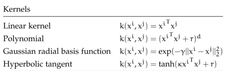
2.6.3 Kernel functions 43 3 d e c i s i o n t r e e s 46
3.1 Decision tree model 48 3.2 Growing decision trees 50
3.2.1 Search among node splitting rules 51 3.2.2 Leaf labelling rules 55
3.2.3 Stop splitting criterion 55 3.3 Right decision tree size 57 3.4 Decision tree interpretation 58 3.5 Multi-output decision trees 60
4 b i a s-va r i a n c e a n d e n s e m b l e m e t h o d s 63 4.1 Bias-variance error decomposition 64 4.2 Averaging ensembles 66
4.2.1 Variance reduction 67
4.2.2 Generic randomization induction
meth-ods 71
4.2.3 Randomized forest model 73 4.3 Boosting ensembles 74
c o n t e n t s xi
4.3.1 Adaboost and variants 76 4.3.2 Functional gradient boosting 79
ii l e a r n i n g i n c o m p r e s s e d s pa c e t h r o u g h r a n d o m p r o j e c t i o n s 84
5 r a n d o m p r o j e c t i o n s o f t h e o u t p u t s pa c e 85 5.1 Methods 87
5.1.1 Multi-output regression trees in randomly pro-jected output spaces 87
5.1.2 Exploitation in the context of tree
ensem-bles 90
5.2 Bias/variance analysis 91 5.2.1 Single random trees. 92
5.2.2 Ensembles of trandom trees. 94 5.3 Experiments 95
5.3.1 Effect of the size q of the Gaussian output
space 95
5.3.2 Systematic analysis over24datasets 96 5.3.3 Input vs output space randomization 100 5.3.4 Alternative output dimension reduction
tech-niques 101
5.3.5 Learning stage computing times 104 5.4 Conclusions 104
6 r a n d o m o u t p u t s pa c e p r o j e c t i o n s f o r g r a d i e n t b o o s t i n g 106
6.1 Introduction 106
6.2 Gradient boosting with multiple outputs 108
6.2.1 Standard extension of gradient boosting to multi-output tasks 108
6.2.2 Adapting to the correlation structure in the output-space 111
6.2.3 Effect of random projections 114 6.2.4 Convergence whenM→∞ 120 6.3 Experiments 121
6.3.1 Experimental protocol 121
6.3.2 Experiments on synthetic datasets with known output correlation structures 123
6.3.3 Effect of random projection 130
6.3.4 Systematic analysis over real world datasets 136 6.4 Conclusions 143 iii e x p l o i t i n g s pa r s i t y f o r g r o w i n g a n d c o m p r e s s -i n g d e c -i s -i o n t r e e s 145 7 `1-b a s e d c o m p r e s s i o n o f r a n d o m f o r e s t m o d -e l s 146
7.1 Compressing tree ensembles by `1-norm regulariza-tion 147
7.2 Empirical analysis 149
7.2.1 Overall performances 150
7.2.2 Effect of the regularization parametert. 151 7.2.3 Influence of the Extra-Tree meta parameters
nmin andM. 152
7.3 Conclusion 153
8 e x p l o i t i n g i n p u t s pa r s i t y w i t h d e c i s i o n t r e e 154
8.1 Tree growing 155
8.1.1 Standard node splitting algorithm 155 8.1.2 Splitting rules search on sparse data 157 8.1.3 Partitioning sparse data 163
8.2 Tree prediction 164 8.3 Experiments 165
8.3.1 Effect of the input space density on synthetic datasets 166
8.3.2 Effect of the input space density on real datasets 167
8.3.3 Algorithm comparison on20newsgroup 169 8.4 Conclusion 172
9 c o n c l u s i o n s 173 9.1 Conclusions 173
9.2 Perspectives and future works 175
9.2.1 Learning in compressed space through random projections 175
9.2.2 Growing and compressing decision trees 176 9.2.3 Learning in high dimensional and sparse
input-output spaces 177 iv a p p e n d i x 179 a d e s c r i p t i o n o f t h e d ata s e t s 180 a.1 Synthetic datasets 180 a.2 Regression datasset 180 a.3 Multi-label dataset 180
a.4 Multi-output regression datasets 181 b i b l i o g r a p h y 184
1
I N T R O D U C T I O N
Progress in information technology enables the acquisition and stor-age of growing amounts of rich data in many domains including science (biology, high-energy physics, astronomy, etc.), engineering (energy, transportation, production processes, etc.), and society (en-vironment, commerce, etc.). Connected objects, such as smartphones, connected sensors or intelligent houses, are now able to record videos, images, audio signals, object localizations, temperatures, social inter-actions of the user through a social network, phone calls or user to computer program interactions such as voice help assistant or web search queries. The accumulating datasets come in various forms such as images, videos, time-series of measurements, recorded trans-actions, text etc. WEB technology often allows one to share locally acquired datasets, and numerical simulation often allows one to gen-erate low cost datasets on demand. Opportunities exist thus for com-bining datasets from different sources to search for generic knowl-edge and enable robust decision.
All these rich datasets are of little use without the availability of au-tomatic procedures able to extract relevant information from them in a principled way. In this context, the field of machine learning aims at developing theory and algorithmic solutions for the extraction of syn-thetic patterns of information from all kinds of datasets, so as to help us to better understand the underlying systems generating these data and hence to take better decisions for their control or exploitation.
Among the machine learning tasks, supervised learning aims at modeling a system by observing its behavior through samples of pairs of inputs and outputs. The objective of the generated model is to predict with high accuracy the outputs of the system given pre-viously unseen inputs. A genomic application of supervised learning would be to model how a DNA sequence, a biological code, is linked to some genetic diseases. The samples used to fit the model are the input-output pairs obtained by sequencing the genome, the inputs, of patients with known medical records for the studied genetic diseases, the outputs. The objective is here twofold: (i) to understand how the DNA sequence influences the appearing of the studied genetic dis-eases and (ii) to use the predictive models to infer the probability of contracting the genetic disease.
The emergence of new applications, such as image annotation, per-sonalized advertising or3D image segmentation, leads to high dimen-sional data with a large number of inputs and outputs. It requires
scalable supervised learning algorithms in terms of computational power and memory space without sacrificing accuracy.
Decision trees (Breiman et al., 1984) are supervised learning mod-els organized in the form of a hierarchical set of questions each one typically based on one input variable leading to a prediction. Used in isolation, trees are generally not competitive in terms of accuracy, but when combined into ensembles (Breiman,2001;Friedman,2001), they yield state-of-the-art performances on standard benchmarks ( Caru-ana et al.,2008;Fernández-Delgado et al.,2014;Madjarov et al.,2012). They however suffer from several limitations that make them not al-ways suited to address modern applications of machine learning tech-niques in particular involving high dimensional input and output spaces.
In this thesis, we identify three main areas where random forest methods could be improved and for which we provide and evalu-ate original algorithmic solutions: (i) learning over high dimensional output spaces, (ii) learning with large sample datasets and stringent memory constraints at prediction time and (iii) learning over high di-mensional sparse input spaces. We discuss each one of these solutions in the following paragraphs.
h i g h d i m e n s i o na l o u t p u t s pa c e s New applications of ma-chine learning have multiple output variables, potentially in very high number (Agrawal et al., 2013; Dekel and Shamir, 2010), asso-ciated to the same set of input variables. A first approach to address such multi-output tasks is the so-called binary relevance / single tar-get method (Spyromitros-Xioufis et al., 2016; Tsoumakas et al.,2009), which separately fits one decision tree ensemble for each output vari-able, assuming that the different output variables are independent. A second approach called multi-output decision trees (Blockeel et al., 2000; Geurts et al., 2006b; Kocev et al., 2013) fits a single decision tree ensemble targeting simultaneously all the outputs, assuming that all outputs are correlated. However in practice, (i) the computational complexity is the same for both approaches and (ii) we have often nei-ther of these two extreme output correlation structures. As our first contribution, we show how to make random forest faster by exploit-ing random projections (a dimensionality reduction technique) of the output space. As a second contribution, we show how to combine gradient boosting of tree ensembles with single random projections of the output space to automatically adapt to a wide variety of corre-lation structures.
m e m o r y c o n s t r a i n t s o n m o d e l s i z e Even with a large num-ber of training samples n, random forest ensembles have good com-putational complexity (O(nlogn)) and are easily parallelizable lead-ing to the generation of very large ensembles. However, the resultlead-ing
1.1 p u b l i c at i o n s 3
models are big as the model complexity is proportional to the num-ber of samplesnand the ensemble size. As our third contribution, we propose to compress these tree ensembles by solving an appropriate optimization problem.
h i g h d i m e n s i o na l s pa r s e i n p u t s pa c e s Some supervised learning tasks have very high dimensional input spaces, but only a few variables have non zero values for each sample. The input space is said to be “sparse”. Instances of such tasks can be found in text-based supervised learning, where each sample is often mapped to a vector of variables corresponding to the (frequency of) occurrence of all words (or multigrams) present in the dataset. The problem is sparse as the size of the text is small compared to the number of possible words (or multigrams). Standard decision tree implementa-tions are not well adapted to treat sparse input spaces, unlike models such as support vector machines (Cortes and Vapnik,1995;Scholkopf
and Smola,2001) or linear models (Bottou,2012). Decision tree imple-mentations are indeed treating these sparse variables as dense ones raising the memory needed. The computational complexity also does not depend upon the fraction of non zero values. As a fourth contri-bution, we propose an efficient decision tree implementation to treat supervised learning tasks with sparse input spaces.
1.1 p u b l i c at i o n s
This dissertation features several publications about random forest algorithms:
• (Joly et al., 2014) A. Joly, P. Geurts, and L. Wehenkel. Random
forests with random projections of the output space for high dimen-sional multi-label classification. In Machine Learning and Knowl-edge Discovery in Databases, pages 607–622. Springer Berlin Heidelberg,2014.
• (Joly et al., 2012) A. Joly, F. Schnitzler, P. Geurts, and L. We-henkel.L1-based compression of random forest models.In European Symposium on Artificial Neural Networks, Computational In-telligence and Machine Learning,2012.
• (Buitinck et al.,2013) L. Buitinck, G. Louppe, M. Blondel, F. Pe-dregosa, A. Mueller, O. Grisel, V. Niculae, P. Prettenhofer, A. Gramfort, J. Grobler, R. Layton, J. Vanderplas, A. Joly, B. Holt, and G. Varoquaux.Api design for machine learning software: experi-ences from the scikit-learn project. arXiv preprint arXiv:1309.0238, 2013.
• H. Fares, A. Joly, and P. Papadimitriou.Scalable Learning of Tree-Based Models on Sparsely Representable Data.
Some collaborations were made during the thesis, but are not dis-cussed within this manuscript:
• (Sutera et al., 2014) A. Sutera, A. Joly, V. François-Lavet, Z. A. Qiu, G. Louppe, D. Ernst, and P. Geurts.Simple connectome infer-ence from partial correlation statistics in calcium imaging.In JMLR: Workshop and Conference Proceedings, pages1–12,2014. • (Delierneux et al., 2015a) C. Delierneux, N. Layios, A. Hego, J.
Huart, A. Joly, P. Geurts, P. Damas, C. Lecut, A. Gothot, and C. Oury. Elevated basal levels of circulating activated platelets predict icu-acquired sepsis and mortality: a prospective study.Critical Care, 19(Suppl1):P29,2015a.
• (Delierneux et al., 2015b) C. Delierneux, N. Layios, A. Hego, J. Huart, A. Joly, P. Geurts, P. Damas, C. Lecut, A. Gothot, and C. Oury.Prospective analysis of platelet activation markers to predict severe infection and mortality in intensive care units. In journal of thrombosis and haemostasis, volume13, pages651–651.
• (Begon et al.,2016) J.-M. Begon, A. Joly, and P. Geurts.Joint
learn-ing and prunlearn-ing of decision forests. In Belgian-Dutch Conference On Machine Learning,2016.
The following article has been submitted:
• C. Delierneux, N. Layios, A. Hego, J. Huart, C. Gosset, C. Lecut, N. Maes, P. Geurts, A. Joly, P. Lancellotti, P. Damas, A. Gothot, and C. Oury. Incremental value of platelet markers to clinical vari-ables for sepsis prediction in intensive care unit patients: a prospective pilot study.
1.2 o u t l i n e
In Part iof this thesis, we start by introducing in Chapter 2 the key concepts about supervised learning: (i) what are the most popular supervised learning models, (ii) how to assess the prediction perfor-mance of a supervised learning model and (iii) how to optimize the hyper-parameters of theses models. We also present some unsuper-vised projection methods, such as random projections, which trans-form the original space to another one. We describe more in detail the decision tree model classes in Chapter 3. More specifically, we describe the methodology to grow and to prune such trees. We also show how to adapt decision tree growing and prediction algorithms to multi-output tasks. In Chapter 4, we show why and how to com-bine models into ensembles either by learning models independently with averaging methods or sequentially with boosting methods.
1.2 o u t l i n e 5
In Partii, we first show how to grow an ensemble of decision trees on very high dimensional output spaces by projecting the original out-put space onto a random sub-space of lower dimension. In Chapter5, it turns out that for random forest models, an averaging ensemble of decision trees, the learning time complexity can be reduced without affecting the prediction performance. Furthermore, it may lead to ac-curacy improvement (Joly et al., 2014). In Chapter 6, we propose to combine random projections of the output space and the gradient tree boosting algorithm, while reducing learning time and automatically adapting to any output correlation structure.
In Part iii, we leverage sparsity in the context of decision tree en-sembles. In Chapter7, we exploit sparsifying optimization algorithms to compress random forest models while retaining their prediction performances (Joly et al., 2012). In Chapter 8, we show how to lever-age input sparsity to speed up decision tree induction.
During the thesis, I made significant contributions to the open source scikit-learn project (Buitinck et al.,2013;Pedregosa et al.,2011) and developed my own open source libraries random-output-trees1
, containing the work presented in Chapter 5and Chapter6, and clus-terlib2
, containing the tools to manage jobs on supercomputers.
1 https://github.com/arjoly/random-output-trees 2 https://github.com/arjoly/clusterlib
2
S U P E R V I S E D L E A R N I N G
Outline
In the field of machine learning, supervised learning aims at find-ing the best function which describes the input-output relation of a system only from observations of this relationship. Supervised learn-ing problems can be broadly divided into classification tasks with discrete outputs and into regression tasks with continuous outputs. We first present major supervised learning methods for both classifi-cation and regression. Then, we show how to estimate their perfor-mance and how to optimize the hyper-parameters of these models. We also introduce unsupervised projection techniques used in con-junction with supervised learning methods.
Supervised learning aims at modeling an input-output system from observations of its behavior. The applications of such learning meth-ods encompass a wide variety of tasks and domains ranging from image recognition to medical diagnosis tools. Supervised learning al-gorithms analyze the input-output pairs and learn how to predict the behavior of a system (see Figure 2.1) by observing its responses, de-scribed by output variables y1,. . .,yd, also called targets, to its envi-ronment described by input variables x1,. . .,xp, also called features. The outcome of the supervised learning is a functionfmodeling the behavior of the system.
Inputs
x1,. . .,xp System
Outputs y1,. . .,yd
Figure2.1: Input-output view of a system.
Supervised learning has numerous applications in the multimedia, in biology, in engineering or in the societal domain:
• Identification of digits from photos, such as house number from street photos or digit post code from letters.
• Automatic image annotation such as detecting tumorous cells or identifying people in photos.
• Detection of genetic diseases from DNA screening.
• Disease diagnostic based on clinical and biological data of a patient.
• Automatic text translation from a source language to a target language such as from French to English.
• Automatic voice to text transcription from audio records. • Market price prediction on the basis of economical and
perfor-mance indicators.
We introduce the supervised learning framework in Section2.1. We describe in Section2.2the most common classes of supervised learn-ing models used to map the outputs of the system to its inputs. We introduce how to assess their performances in Section 2.3, how to compare the model predictions to a ground truth in Section 2.4 and how to select the best hyper-parameters of such models in Section2.5. We also show some input space projection methods in Section2.6, of-ten used in combination with supervised learning models improving the computational time and / or the accuracy of the model.
2.1 i n t r o d u c t i o n
The goal of supervised learning is to learn the functionfmapping an input vectorx= (x1,. . .,xp)of a system to a vector of system outputs
y = (y1,. . .,yd), only from observations of input-output pairs. The set of possible input (resp. output) vectors form the input space X (resp. output spaceY).
Once we have identified the input and output variables, we start to collect input-output pairs, also called samples. Table 2.1 displays 5 samples collected from a system with 4 inputs and 3 outputs. We distinguish three types of variables: binary variables taking only two different values, like the variablesx1andy1; categorical variables tak-ing two or more possible values, like variablesx2andy2, and numer-ical variables having numernumer-ical values, like x2, x4 and y3. A binary variable is also a categorical variable. For simplicity, we will assume in the following without loss of generality that binary and categorical variables have been mapped from the set of theirkoriginal values to a set of integers of the same cardinality {0,. . .,k−1}.
Table2.1: A dataset formed of samples of pairs of four inputs and three outputs. x1 x2 x3 x4 y1 y2 y3 0 0.25 A 0.25 True Small 1.8 ? −2 B 3. True Average 1.7 0 3 C 2. False ? 1.65 1 10.7 ? −3. False Big 1.59 1 0. A 2. False Big ?
2.1 i n t r o d u c t i o n 9
When we collect data, some input and/or output values might be missing or unavailable. Tasks with missing input values are said to have missing data. Missing values are marked by a “?” in Table 2.1.
We classify supervised learning tasks into two main families based on their output domains. Classification tasks have either binary out-puts as in disease prediction (y∈{Healthy,sick}) or categorical out-puts as in digits recognition (y ∈ {0,. . .,9}). Regression tasks have numerical outputs (y∈R) such as in house price predictions. A clas-sification task with only one binary output (resp. categorical output) is called a binary classification task (resp. multi-class classification task). A multi-class classification task is assumed to have more than two classes, otherwise it is a binary classification task. In the pres-ence of multiple outputs, we further distinguish multi-label classifi-cation tasks which associate multiple binary output values to each input vector. In the multi-label context, the output variables are also called “labels” and the output vectors are called “label set”. From a modeling perspective, multi-class classification tasks are multi-label classification problems whose labels are mutually exclusive. Table2.2 summarizes the different supervised learning tasks.
Table2.2: The output domain determines the supervised learning task.
Supervised learning task Output domain
Binary classification Y={0,1}
Multi-class classification Y={0,1,. . .,k−1}withk>2 Multi-label classification Y={0,1}dwithd>1
Multi-output multi-class classification Y={0,1,. . .,k−1}d withk > 2,d > 1
Regression Y=R
Multi-output regression Y=Rdwithd>1
We will denote by X an input space, and by Y an output space. We denote byPX,Y the joint (unknown) sampling density over X×Y. Superscript indices (xi,yi) denote (input, output) vectors of an obser-vationi∈{1,. . .,n}. Subscript indices (e.g.xj,yk) denote components of vectors. With these notations supervised learning can be defined as follows:
Supervised learning
Given a learning sample (xi,yi)∈(X×Y)n
i=1 of nobservations in the form of input-output pairs, a supervised learning task is defined as searching for a functionf∗ :X→Yin a hypothesis spaceH ⊂YX
Table2.3: Common losses to measure the discrepancy between a ground truth yand either a prediction or a scorey0. In classification, we assume here that the ground truth yis encoded with{−1,1} val-ues.
Regression loss
Square loss `(y,y0) = 12(y−y0)2 Absolute loss `(y,y0) =|y−y0| Binary classification loss
0-1loss `(y,y0) =1(y6=y0) Hinge loss `(y,y0) =max(0,1−yy0) Logistic loss `(y,y0) =log(1+exp(−2yy0))
that minimizes the expectation of some loss function` :Y×Y→ R+ over the joint distribution of input / output pairs:
f∗=arg min
f∈HEPX,Y{`(f(x),y)}. (
2.1)
The choice of the loss function ` depends on the property of the supervised learning task (see Table 2.3for their definitions):
• In regression (Y = R), we often use the squared loss, except when we want to be robust to the presence of outliers, samples with abnormal output values, where we prefer other losses such as the absolute loss.
• In classification tasks (Y = {0,. . .,k−1}), the reported perfor-mance is commonly the average0−1 loss, called the error rate. However, the model does not often directly minimize the0−1 loss as it leads to non convex and non continuous optimization problems with often high computational cost. Instead, we can relax the multi-class or the binary constraint by optimizing a smoother loss such as the hinge loss or the logistic loss. To get a binary or multi-class prediction, we can threshold the predicted valuef(x).
Figure 2.2 plots several loss discrepancies `(1,y0) whenever the ground truth is y = 1 d as a function of the value y0 predicted by the model. The 0−1 loss is a step function with a discontinuity at y0 =1. The hinge loss has a linear behavior whenevery061and is a constant withy0>1. The logistic loss strongly penalizes any mistake and is zero only if the model is correct with an infinite score. The plot also highlights that we can use regression losses for classification
2.2 c l a s s e s o f s u p e r v i s e d l e a r n i n g a l g o r i t h m s 11
2
2
Predicted value
y
00.0
4.5
Lo
ss
d
is
cr
ep
an
cy
`
(1
,y
0)
0-1 loss
Absolute loss
Hinge loss
Logistic loss
Squared loss
Figure2.2: Loss discrepancies `(1,y0) with y = 1. (Adapted from (Hastie et al.,2009))
tasks. It shows that regression losses penalize any predicted valuey0 different from the ground truth y. However, this is not always the desired behavior. For instance whenever y= 1 (resp.y = 0), regres-sion losses penalize any score greater than y0> 1(resp. smaller than y0 < 0), while the model truly believes that the output is positive (resp. negative). This is often the reason why regression losses are avoided for classification tasks.
2.2 c l a s s e s o f s u p e r v i s e d l e a r n i n g a l g o r i t h m s
Supervised learning aims at finding the best functionfin a hypothe-sis space H to model the input-output function of a system. If there is no restriction on the hypothesis space H, the model f can be any functionf∈YX.
Consider a binary functionfwhich haspbinary inputs. The binary function is uniquely defined by knowing the output values of the 2p possible input vectors. The hypothesis space of all binary functions contains 22p binary functions. If we observe ndifferent input-output pair assignments, there remain 22p−n possible binary functions. For a binary function of p = 5 inputs, we have 225 = 4294967296 possi-ble binary functions. If we observe n = 16 input-output pair assign-ments among the25 =32possible ones, we still have225−16 =65536 possible binary functions. The number of possible functions highly increases with the cardinality of each variable. The hypothesis space will be even larger with a stochastic function, where different output values are possible for each possible input assignment.
By making assumptions on the model class H, we can largely re-duce the size of the hypothesis space. For instance in the previous example, if we assume that 2 out of the5 binary input variables are independent of the output, there remain223=256possible functions.
The correct function would be uniquely identified by observing the8 possible assignments.
Given the data stochasticity, those model classes can directly model the input-output mapping f:X→ Y, but also the conditional proba-bilityP(y|x)and predictions are made through
f(x) =arg min ˆ y∈YEy|x[L(y, ˆy)] =arg minyˆ Z Y L(y, ˆy)dP(y|x). (2.2) We will present some of the most popular model classes: linear models in Section 2.2.1; artificial neural networks in Section 2.2.2 which are inspired from the neurons in the brain; neighbors-based models in Section2.2.3which find the nearest samples in the training set; decision tree based-models in Section2.2.4(and in more details in Chapter3). Note that we introduce ensemble methods in Section2.2.4 and discuss them more deeply in Chapter4.
2.2.1 Linear models
Let us denote byx∈Rp=h
x1 . . . xp iT
a vector of input variables. A linear model ˆfis a model having the following form
ˆ f(x) =β0+ p X j=1 βjxj= h 1 xT i β
where the vectorβ∈R1+pis a concatenation of the interceptβ 0 and the coefficientsβj.
Given a set of n input-output pairs {(xi,yi) ∈ (X,Y)}n
i=1, we re-trieve the coefficient vector β of the linear model by minimizing a loss`: Y× Y→R+: min β n X i=1 `(yi, ˆf(xi)) =min β n X i=1 `(yi,h1 xiTiβ). (2.3)
With the square loss`(y,y0) = 21(y−y0)2, there exists an analytical solution to Equation 2.3 called ordinary least squares. Let us denote by X ∈ Rn×(1+p) the concatenation of the input vectors with a first column ofXfull of ones to model the interceptβ0 and byy∈Rnthe concatenation of the output values. We can now express the sum of squares in matrix notation:
n X i=1 `(y, ˆf(xi)) = 1 2 n X i=1 (yi−fˆ(xi))2 (2.4) = 1 2(y−Xβ) T( y−Xβ) (2.5)
2.2 c l a s s e s o f s u p e r v i s e d l e a r n i n g a l g o r i t h m s 13
The first order differentiation of the sum of squares with respect toβ yields to ∂ ∂β n X i=1 `(y, ˆf(xi)) =XT(y−Xβ). (2.6)
The vector minimizing the square loss is thus
β= (XTX)−1XTy. (2.7)
The solution exists only ifXTXis invertible.
Whenever the number of inputs plus onep+1is greater than the number of samples n, the analytical solution is ill posed as the ma-trix XTX is rank deficient (rank(XTX) < p+1). To ensure a unique solution, we can add a regularization penalty R with a multiplying constantλ∈R+ on the coefficients βof the linear model:
min β n X i=1 L(yi,β0+ p X j=1 βjxij) +λR(β1, . . .,βp). (2.8)
With a`2-norm constraint on the coefficients, we transform the or-dinary least square model into a ridge regression model (Hoerl and Kennard,1970): min β n X i=1 yi−β0− p X j=1 βjxij 2 +λ p X j=1 β2j. (2.9)
One can show (see Section 3.4.1of (Hastie et al., 2009)) that the con-stant λcontrols the maximal value of all coefficients βj in the ridge regression solution.
With a`1-norm constraint (R(β1, . . .,βp) =
Pp
j=1|βj|) on the coef-ficientβ1,. . .,βp, we have the Lasso model (Tibshirani,1996b):
min β n X i=1 yi−β0− p X j=1 βjxij 2 +λ p X j=1 |βj|. (2.10)
Contrarily to the ridge regression, the Lasso has no closed formed analytical solution even though the resulting optimization problem remains convex. However, we gain that the`1-norm penalty sparsifies the coefficientsβj of the linear model. If the constantλtends towards infinity, all the coefficients will be zero βj = 0. While with λ = 0, we have the ordinary least square formulation. Withλmoving from +∞ to 0, we progressively add variables to the linear model with a magnitude Ppj=1|βj| depending on λ. The monotone Lasso (Hastie et al., 2007) further restricts the coefficient to monotonous variation with respect toλand has been shown to perform better whenever the input variables are correlated.
(a)
(b) Original input space (c) Non-linear transformation
Figure2.3: The logistic linear model on the bottom left is unable to find a separating hyperplane. If we fit the linear model on the distance from the center of circle, we separate perfectly both classes as shown in the bottom right.
A combination of the`1-norm and the`2-norm constraints on the coefficients is called an elastic net penalty (Zou and Hastie, 2005). It shares both the property of the Lasso and the ridge regression: sparsely selecting coefficients as in Lasso and considering groups of correlated variables together as in the ridge regression. With a care-ful design of the penalty term R, we can enforce further properties such as selecting variables in groups of pre-defined variables with the group Lasso (Meier et al.,2008;Yuan and Lin,2006) or taking into account the variable locality in the coefficient vector βwhile adding a new variable to the linear model with the fused Lasso (Tibshirani et al.,2005).
By selecting an appropriate loss and penalty term, we have a wide variety of linear models at our disposal with different properties. In regression, an absolute loss leads to the least absolute deviation al-gorithm (Bloomfield and Steiger, 2012) which is robust to outliers. In classification, we can use a logistic loss to model the class prob-ability distribution leading to the logistic regression model. With a hinge loss, we aim at finding a hyperplane which maximizes the sep-arations between the classes leading to the support vector machine algorithm (Cortes and Vapnik,1995).
A linear model can handle non linear problems by applying first a non linear transformation to the input space X. For instance, con-sider the classification task of Figure 2.3awhere each class is located on a concentric circle. Given the non linearity of the problem, we can not find a straight line separating both classes in the cartesian plane
2.2 c l a s s e s o f s u p e r v i s e d l e a r n i n g a l g o r i t h m s 15
as shown in Figure 2.3b. If instead we fit a linear model on the dis-tance from the origin
q x2
1+x22 as illustrated in Figure2.3c, we find a model separating perfectly both classes. We often use linear mod-els in conjunction with kernel functions (presented in Section 2.6.3), which provide a range of ways to achieve non-linear transformations of the input space.
2.2.2 (Deep) Artificial neural networks
An artificial neural network is a statistical model mimicking the struc-ture of the brain and composed of artificial neurons. A neuron, as shown in Figure 2.4a, is composed of three parts: the soma, the cell body, processes the information from its dendrites and transmits its results to other neurons through the axon, a nerve fiber. An artificial neuron follows the same structure (see Figure 2.4b) replacing biolog-ical processing by numerbiolog-ical computations. The basic neuron ( Rosen-blatt,1958) used for supervised learning consists in a linear model of parametersβ∈Rp+1followed by an activation function φ:
ˆ fneuron(x) =φ β0+ p X j=1 βjxj .
The activation function replicates artificially the non linear activa-tion of real neurons. It is a scalar funcactiva-tion such as a hyperbolic tan-gent φ(x) = tanh(x), a sigmoid φ(x) = (1+e−x)−1 or a rectified linear functionφ(x) =max(0,x).
(a) Biological neuron
ˆ y Output φ Σ 1 Inputs β0 x1 β1 x2 β2 (b) Artificial neuron
Figure2.4: A biological neuron (on the left) and an artificial neuron (on the right).
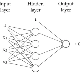
More complex artificial neural networks are often structured into layers of artificial neurons. The inputs of a layer are the input vari-ables or the outputs of the previous layer. Each neuron of the layer has one output. The neural network is divided into three parts as in Figure2.5: the first and last layers are respectively theinput layerand theoutput layer, while the layers in between are thehidden layers. The hidden layer of Figure 2.5 is called a fully connected layer as all the
neurons (here the input variables) from the previous layer are con-nected to each neuron of the layer. Other layer structures exist such as convolutional layers (Krizhevsky et al., 2012; LeCun et al., 2004) which mimic the visual cortex (Hubel and Wiesel,1968). A network is not necessarily feed forward, but can have a more complex topol-ogy for example recurrent neural networks (Boulanger-Lewandowski et al.,2012; Graves et al., 2013) mimic the brain memory by forming internal cycles of neurons. Neural networks with many layers are also known (LeCun et al.,2015) as deep neural networks.
1 x1 x2 x3 1 ˆ y Hidden layer Input layer Output layer
Figure2.5: A neural network with an input layer, a fully connected hidden layer and an output layer.
Artificial neurons form a graph of variables. Through this repre-sentation, we can learn such models by applying gradient based op-timization techniques (Bengio,2012;Glorot and Bengio,2010;LeCun
et al., 2012) to find the coefficient vector associated to each neuron minimizing a given loss function.
2.2.3 Neighbors based methods
Thek-nearest neighbors model is defined by a distance metricdand a set of samples. At learning time, those samples are stored in a database. We predict the output of an unseen sample by aggregat-ing the outputs of thek-nearest samples in the input space according to the distance metricd, withkbeing a user-defined parameter.
More precisely, given a training set (xi,yi)∈(X×Y)n
i=1 and a distance measure d : X×X → R+, an unseen sample with value in the input space x is assigned a prediction through the following procedure:
1. Compute the distancesd(xi,x)in the input space,∀i=1,. . .,n, between the training samplesxiand the input vectorx.
2. Search for theksamples in the training set which have the small-est distance to the vectorx.
2.2 c l a s s e s o f s u p e r v i s e d l e a r n i n g a l g o r i t h m s 17
3. In classification, compute the proportion of samples of each class among these k-nearest neighbors: the final prediction is the class with the highest proportion. This corresponds to a majority vote over the k nearest neighbors. In regression, the prediction is the average output of thek-nearest neighbors. Thek-nearest neighbor method adapts to a wide variety of scenar-ios by selecting or by designing a proper distance metric such as the euclidean distance or the Hamming distance.
2.2.4 Decision tree models
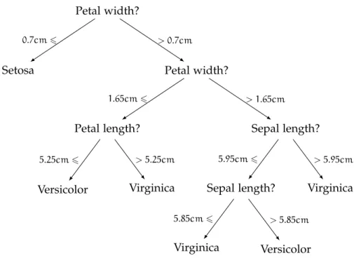
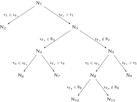
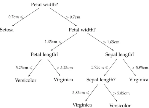
A decision tree model is a hierarchical set of questions leading to a prediction. The internal nodes, also called test nodes, test the value of a feature. In Figure 2.6, the starting node, also called root node, tests whether the feature “Petal width” is bigger or smaller than 0.7cm. According to the answer, you follow either the right branch (> 0.7cm) leading to another test node or the left branch (6 0.7cm) leading to an external node, also called a leaf. To predict an unseen sample, you start at the root node and follow the tree structure until reaching a leaf labelled with a prediction. With the decision tree of Figure2.6, an iris with petal width smaller than0.7cmis an iris Setosa.
Petal width? Setosa 0.7cm6 Petal width? Petal length? Versicolor 5.25cm6 Virginica > 5.25cm 1.65cm6 Sepal length? Sepal length? Virginica 5.85cm6 Versicolor > 5.85cm 5.95cm6 Virginica > 5.95cm > 1.65cm > 0.7cm
Figure2.6: A decision tree classifying iris flowers into its Setosa, Versicolor or Virginica varieties according to the width and length of its petals and sepals.
A classification or a regression tree (Breiman et al., 1984) is built using all the input-output pairs((xi,yi)∈(X×Y))ni=1 as follows: for each test node, the best split(Sr,Sl)of the local subsampleSreaching
the node is chosen among the p input features combined with the selection of an optimal cut point. The best sample split (Sr,Sl) of S minimizes the average reduction of impurity
∆I((yi)i∈S,(yi)i∈Sl,(yi)i∈Sr) =I((yi)i∈S) −| Sl| |S|I((y i) i∈Sl) −| Sr| |S| I((y i) i∈Sr), (2.11) whereIis the impurity of the output such as the entropy in classifica-tion or the variance in regression. The decision tree growth continues until we reach a stopping criterion such as no impurityI((yi)i∈S) =0.
To avoid over-fitting, we can stop earlier the tree growth by adding further stopping criteria such as a maximal depth or a minimal num-ber of samples to split a node.
Instead of a single decision tree, we often train an ensemble of such models:
• Averaging-based ensemble methods grow an ensemble by ran-domizing the tree growth. The random forest method (Breiman, 2001) trains decision trees on bootstrap copies of the training set, i.e. by sampling with replacement from the training dataset, and it randomizes the best split selection by searching this split amongkout of thepfeatures at each nodes (k6p).
• Boosting-based methods (Freund and Schapire,1997;Friedman, 2001) build iteratively a sequence of weak models such as shal-low trees which perform only slightly better than random guess-ing. Each new model refines the prediction of the ensemble by focusing on the wrongly predicted training input-output pairs. We further discuss decision tree models in Chapter3and ensemble methods in Chapter4.
2.2.5 From single to multiple output models
With multiple outputs supervised learning tasks, we have to infer the values of a set of d output variables y1,. . .,yd (instead of a single one) from a set of p input variables x1,. . .,xp. We hope to improve the accuracy and / or computational performance by exploiting the correlation structure between the outputs. There exist two main ap-proaches to solve multiple output tasks: problem transformation pre-sented in Section 2.2.5.1 and algorithm adaptation in Section2.2.5.2. We present here a non exhaustive selection of both approaches. The interested reader will find a broader review of the multi-label litera-ture in (Gibaja and Ventura, 2014; Madjarov et al., 2012; Tsoumakas
et al.,2009;Zhang and Zhou,2014) and of the multi-output regression literature in (Borchani et al.,2015;Spyromitros-Xioufis et al.,2016).
2.2 c l a s s e s o f s u p e r v i s e d l e a r n i n g a l g o r i t h m s 19
2.2.5.1 Problem transformation
The problem transformation approach transforms the original multi-output task into a set of single multi-output tasks. Each of these single output tasks is then solved by classical classifiers or regressors. The possible output correlations are exploited through a careful reformu-lation of the original task.
i n d e p e n d e n t e s t i m at o r s The simplest way to handle multi-output learning is to treat all multi-outputs in an independent way. We break the prediction of the d outputs intod independent single out-put prediction tasks. A model is fitted on each outout-put. At prediction time, we concatenate the predictions of thesedmodels. This is called the binary relevance method (Tsoumakas et al., 2009) in multi-label classification and the single target method (Spyromitros-Xioufis et al., 2016) in multi-output regression. Since we consider the outputs inde-pendently, we neglect the output correlation structure. Some methods may however benefit from sharing identical computations needed for the different outputs. For instance, thek-nearest neighbor method can share the search for the k-nearest neighbors in the input space, and the ordinary linear least squares method can share the computation of (XTX)−1XT in Equation2.7.
e s t i m at o r c h a i n If the outputs are dependent, the model of a single output might benefit from the values of the correlated outputs. In the estimator chain method, we sequentially learn a model for each output by providing the predictions of the previously learnt models as auxiliary inputs. This is called a classifier chain (Read et al.,2011) in classification and a regressor chain (Spyromitros-Xioufis et al., 2016) in regression.
More precisely, the estimator chain method first generates an order o on the outputs for instance based on prior knowledge, the output density, the output variance or at random. Then with the training samples and the output order o, it sequentially learns d estimators: the l-th estimator fol aims at predicting the ol-th output using as inputs the concatenation of the input vectors with the predictions of the models learnt for the l−1 previous outputs. To reduce the model variance, we can generate an ensemble of estimator chains by randomizing the chain order (and / or the underlying base estimator), and then we average their predictions.
In multi-label classification,Cheng et al.(2010) formulates a Bayes optimal classifier chain by modeling the conditional probability of PY|X(y|x). Under the chain rule, we have
PY|X(y|x) =PY 1|X(y1|x) d Y j=2 PY j|X,Y1,...,Yj−1(yj|x,y1,. . .,yj−1). (2.12)
Each estimator of the chain approximates a probability factor of the chain rule decomposition. Using the estimation of PY|X made by the chain and a given loss function`, we can perform Bayes optimal pre-diction:
h∗(x) =arg min
y0 EY|X`(y 0
,y). (2.13)
e r r o r c o r r e c t i n g c o d e s Error correcting codes are techniques from information and coding theory used to properly deliver a mes-sage through a noisy channel. It first codes the original mesmes-sage, and then corrects the errors made during the transmission at decoding time. This idea have been applied to multi-class classification ( Diet-terich and Bakiri;Guruswami and Sahai,1999), multi-label classifica-tion (Cisse et al.,2013;Ferng and Lin,2011;Guo et al.,2008;Hsu et al., 2009;Kajdanowicz and Kazienko,2012; Kapoor et al.,2012;Kouzani
and Nasireding, 2009; Zhang and Schneider,2011) and multi-output regression (Tsoumakas et al., 2014; Yu et al., 2006) tasks by viewing the predictions made by the supervised learning model(s) as a mes-sage transmitted through a noisy channel. It transforms the original task by encoding the output values with a binary error correcting code or output projections. One classifier is then fitted for each bit of the code or output projection. At prediction time, we concatenate the predictions made by each estimator and decode them by solving the inverse problem. Note that the output coding might also have for objective to reduce the dimensionality of the output space (Hsu et al., 2009;Kapoor et al.,2012).
pa i r w i s e c o m pa r i s o n s In multi-label tasks, the ranking by pair-wise comparison approach (Hüllermeier et al.,2008) aims to generate a ranking of the labels by making all the pairwise label comparisons. The original tasks is transformed into d(d−1)/2 binary classifica-tion tasks where we compare if a given label is more likely to ap-pear than another label. The datasets comparing each label pair is obtained by collecting all the samples where only one of the outputs is true, but not both. This approach is similar to the one-versus-one approach (Park and Fürnkranz,2007) in multi-class classification task, however we can not directly transform the ranking into a prediction, i.e. label set. To decrease the prediction time, alternative ranking con-struction schemes have been proposed (Mencia and Fürnkranz,2008;
Mencía and Fürnkranz,2010) requiring less thand(d−1)/2classifier predictions.
The Calibrated label ranking method (Brinker et al., 2006;
Fürnkranz et al., 2008) extends the previous approach by adding a virtual label which will serve as a split point between the true and the false labels. For each label, we add a new tasks using all the samples comparing the labelito the virtual label whose value is the opposite of the labeli. To thed(d−1)/2tasks, we effectively adddtasks.
2.2 c l a s s e s o f s u p e r v i s e d l e a r n i n g a l g o r i t h m s 21
l a b e l p o w e r s e t For multi-label classification tasks, the label power set method (Tsoumakas et al., 2009) encodes each label set in the training set as a class. It transforms the original task into a multi-class classification task. At prediction time, the class predicted by the multi-class classifier is decoded thanks to the one-to-one map-ping of the label power set encoding. The drawback of this approach is to generate a large number of classes due to the large number of possible label sets. Fornsamples anddlabels, the maximal number of classes is max(2d,n). This leads to accuracy issues if some label sets are not well represented in the training set. To alleviate the explo-sion of classes, rakel (Tsoumakas and Vlahavas, 2007) generates an ensemble of multi-class classifiers by subsampling the output space and then applying the label power set transformation.
2.2.5.2 Algorithm adaptation
The algorithm adaptation approach modifies existing supervised learning algorithms to handle multiple output tasks. We show here how to extend the previously presented models classes to multi-output regression and to multi-label classification tasks.
l i n e a r-b a s e d m o d e l s Linear-based models have been adapted to multi-output tasks by reformulated their mathematical formu-lation using multi-output losses and (possibly) regularization con-straints enforcing assumptions on the input-output and the output-output correlation structures. The proposed methods are based for instance on extending least-square regression (Baldassarre et al.,2012;
Breiman and Friedman,1997;Dayal and MacGregor,1997;Evgeniou
et al., 2005; Similä and Tikka, 2007; Zhou and Tao, 2012) (with pos-sibly regularization), canonical correlation analysis (Izenman, 1975;
Van Der Merwe and Zidek, 1980), support vector machine (Elisseeff
and Weston, 2001; Evgeniou and Pontil, 2004; Evgeniou et al., 2005;
Jiang et al., 2008; Xu, 2012), support vector regression (Liu et al., 2009; Sánchez-Fernández et al., 2004; Vazquez and Walter, 2003; Xu
et al., 2013), and conditional random fields (Ghamrawi and
McCal-lum,2005).
(d e e p) a r t i f i c i a l n e u r a l n e t w o r k s Neural networks han-dles multi-output tasks by having one node on the output layer per output variable. The network minimizes a global error function de-fined over all the outputs (Ciarelli et al.,2009;Nam et al.,2014;Specht, 1991; Zhang, 2009; Zhang and Zhou, 2006). The output correlation are taken into account by sharing the input and the hidden layers between all the outputs.
n e a r e s t n e i g h b o r s Thek-nearest neighbors algorithm predicts an unseen sample x by aggregating the output value of the k
near-est neighbors of x. This algorithm is adapted to multi-output tasks by sharing the nearest neighbors search among all outputs. If we just share the search, this is called binary relevance ofk-nearest neighbors in classification and single target ofk-nearest neighbors in regression. Multi-output extensions of thek-nearest neighbors modifies how the output values of the nearest neighbors are aggregated for the pre-dictions for instance it can utilize the maximum a posteriori princi-ple (Cheng and Hüllermeier, 2009; Younes et al., 2011; Zhang and
Zhou,2007) or it can re-interpret the output aggregation as a ranking problem (Brinker and Hüllermeier,2007;Chiang et al.,2012),
d e c i s i o n t r e e s The decision tree model is a hierarchical struc-ture partitioning the input space and associating a prediction to each partition. The growth of the tree structure is done by maximizing the reduction of an impurity measure computed in the output space. When the tree growth is stopped at a leaf, we associate a prediction to this final partition by aggregating the output values of the train-ing samples. We adapt the decision tree algorithm to multi-output tasks in two steps (Blockeel et al.,2000;Clare and King,2001;De’Ath, 2002; Noh et al., 2004;Segal,1992;Vens et al.,2008;Zhang, 1998): (i) multi-output impurity measures are used to grow the structure as the sum over the output space of the entropy or the variance; (ii) the leaf predictions are obtained by computing a constant minimizing a multi-output loss function such as the `2-norm loss in regression or the Hamming loss in classification. We discuss in more details how to adapt the decision tree algorithm to multi-output tasks in Section3.5.
Instead of growing a single decision tree, they are often combined together to improve their generalization performance. Random forest models (Breiman,2001;Geurts et al.,2006a) averages the predictions of several randomized decision trees and has been studied in the con-text of multi-output learning (Joly et al.,2014;Kocev et al.,2007,2013;
Madjarov et al.,2012;Segal and Xiao,2011).
e n s e m b l e s Ensemble methods aggregate the predictions of mul-tiple models into a single one so to improve its generalization perfor-mance. We discuss how the averaging and boosting approaches have been adapted to multi-output supervised learning tasks.
Averaging ensemble methods have been straightforwardly adapted by averaging the prediction of multi-output models. Instead of averag-ing scalar predictions, it averages (Joly et al.,2014;Kocev et al.,2007, 2013; Madjarov et al., 2012; Segal and Xiao, 2011) the vector predic-tions of each model of the ensemble. If the learning algorithm is not inherently multi-output, we could use one the problem transforma-tion techniques as in rakel (Tsoumakas and Vlahavas, 2007), which uses the label power set transformation, or ensemble of estimator chain (Read et al.,2011).
2.3 e va l uat i o n o f m o d e l p r e d i c t i o n p e r f o r m a n c e 23
Boosting ensembles are grown by sequentially adding weak models minimizing a selected loss, such as the Hamming loss (Schapire and Singer, 2000), the ranking loss (Schapire and Singer, 2000), the `2 -norm loss (Geurts et al.,2006b) or any differentiable loss function (see Chapter6).
2.3 e va l uat i o n o f m o d e l p r e d i c t i o n p e r f o r m a n c e
For a given supervised learning modelf trained on a set of samples (xi,yi)∈(X×Y)ni=1, we want a model having good generalization able to predict unseen samples. Otherwise said, the model f should have minimal generalization error over the input-output pair distri-bution, where the generalization error is defined as:
Generalization error=EPX,Y{`(f(x),y)} (2.14) for a given loss function`:Y×Y→R+.
Evaluating Equation2.14is generally unfeasible, except in the rare cases where (i) the input-output distributionPX,Yis fully known and (ii) for restricted classes of models. In practice, neither of these condi-tions are met. However, we still need a principle way to approximate the generalization error.
A first approach to approximate Equation2.14is to evaluate the er-ror of the modelfon the training samplesL= (xi,yi)∈(X×Y)ni=1 leading to the resubstitution error:
Resubstitution error= 1 |L| n X (x,y)∈L `(f(x),y) (2.15)
A model with a high resubstitution error often has a high general-ization error and indeed underfits the data. The linear model shown in Figure2.7aunderfits the data as it is not complex enough to fit the non linear data (here a second degree polynomial). Instead, we can fit a high order polynomial model to have a zero resubstitution error as illustrated in Figure2.7b. This complex model has poor generaliza-tion error as it perfectly fits the noisy samples unable to retrieve the second order parabola. Such overly complex models with zero resub-stitution error and non zero generalization error are said to overfit the data. Since a zero resubstitution error does not imply a low gen-eralization error, it is a poor proxy of the gengen-eralization error.
Since we assess the quality of the model with the training sam-ples, the resubstitution error is optimistic and biased. Furthermore, it favors overly complex models (as depicted in Figure 2.7). To im-prove the approximation of the generalization error, we need to use techniques which avoid to use the training samples for performance evaluation. They are either based on sample partitioning methods, such as hold out methods and cross validation techniques, or sample
True function Model prediction Noisy training samples
(a) Under-fitting (b) Over-fitting
Figure2.7: The linear model on the left figure underfits the training samples, while the high order polynomial model on the right overfits the training samples.
resampling methods, such as bootstrap estimation methods. Since the amount of available data and time are fixed for both the model train-ing and the model assessment, there is a trade-off between (i) the quality of the error estimate, (ii) the number of samples available to learn a model and (iii) the amount of computing time available for the whole process.
The hold out evaluation method splits the samples into a training setLS, also called learning set, and a testing setT Scommonly with a ratio of2/3-1/3. The hold out error is given by
Hold out error= 1 |T S|
X (x,y)∈T S
`(f(x),y). (2.16)
This methods requires a high number of samples as a large part of the data is devoted to the model assessment impeding the model training. If too few samples are allocated to the testing set, the hold out esti-mate becomes unreliable as its confidence intervals widen (Kohavi et al.,1995). Since the hold out error is a random number depending on the sample partition, we can improve the error estimation by (i) generating B random partitions (LSb,T Sb)Bb=1 of the available sam-ples, (ii) fitting a modelfb on each learning set LSb and (iii) averag-ing the performance of theBmodels over their respective testing sets T Sb:
Random subsampling error= 1
B B X b=1 1 |T Sb| X (x,y)∈T Sb `(fb(x),y). (2.17) To improve the data usage efficiency, we can resort to cross-validation methods, also called rotation estimation, which split the samples into k folds {T S1,. . .,T Sk} approximately of the same size. Cross validation methods average the performance of k models
2.3 e va l uat i o n o f m o d e l p r e d i c t i o n p e r f o r m a n c e 25
(fl)kl=1 each tested on one of thek folds and trained using thek−1 remaining folds: CV error= 1 k k X l=1 1 |T Sl| X (x,y)∈T Sl `(fl(x),y). (2.18)
The number of foldskis usually 5or 10. If kis equal to the number of samples (k=n), it is called leave-one-out cross validation.
Given that the folds do not overlap for cross validation methods, we are tempted to assess the performance over the pooled cross val-idation estimates with a givenmetricobtained by concatenating the predictions made by each modelflover each of thek-folds
Pooled CV error=metric(f1(x),y)(x,y)∈T S1_. . ._(fk(x),y)(x,y)∈T Sk
, (2.19) where _ is the concatenation operator. There is no difference for sample-wise losses such as the square loss. However, this is not the case for metrics comparing a whole set of predictions to their ground truth. Depending on the metrics, it has been showed that pooling may or may not biase the error estimation (Airola et al.,2011;Forman and
Scholz,2010;Parker et al.,2007).
We can improve the quality of the estimate by repeating the cross validation procedures overBdifferentk-fold partitions, averaging the performance of the modelsfb,l over each associated testing setT Sb,l:
Repeated CV error= 1 Bk B X b=1 k X l=1 1 |T Sb,l| X (x,y)∈T Sb,l `(fb,l(x),y). (2.20)
If all combinations are tested exhaustively as in the leave-one-out case, it is called complete cross validation. Since it is often too expen-sive (Kohavi et al.,1995), we can instead draw several sets of folds at random.
The bootstrap method (Efron, 1983) draws B bootstrap datasets {B1,. . .,BB}by sampling with replacement nsamples from the origi-nal dataset of size n. Each samples has a probability of 1− (1−n1)n to be selected in a bootstrap which is approximately0.632for largen. A first approach to estimate the error is to train a modelfb on each bootstrap dataset and use the original dataset as a testing set:
Bootstrap error= 1 nB B X b=1 X (x,y)∈Bb `(fb(x),y). (2.21) This leads to over optimistic results, given the overlap between the training and the test data.
A better approach (discussed in Chapter7.11of (Hastie et al.,2009)) is to imitate cross validation methods by fitting on each bootstrap