Super-resolution land cover mapping by deep learning

Super-resolution land cover mapping by deep learning

Feng Ling

_{, Giles Foody}

1. Key Laboratory of Monitoring and Estimate for Environment and Disaster of Hubei Province, Institute of Geodesy and Geophysics, Chinese Academy of Sciences, Wuhan 430077, China

2. Sino-Africa Joint Research Centre, Chinese Academy of Sciences, Wuhan 430077, China

3. School of Geography, University of Nottingham, Nottingham NG7 2RD, U.K.

Super-resolution land cover mapping by deep learning

Abstract: Super-resolution mapping (SRM) is a technique to estimate a fine spatial resolution land cover map from coarse spatial resolution fractional proportion images. SRM is often based explicitly on the use of a spatial pattern model that represents the land cover mosaic at the fine spatial resolution. Recently developed deep learning methods have considerable potential as an alternative approach for SRM, based on learning the spatial pattern of land cover from existing fine resolution data such as land cover maps. This letter proposes a deep learning based SRM algorithm (DeepSRM). A deep convolutional neural network was first trained to estimate a fine resolution indicator image for each class from the coarse resolution fractional image, and all indicator maps were then combined to create the final fine resolution land cover map based on the maximal value strategy. The results of an experiment undertaken with simulated images show that DeepSRM was superior to conventional hard classification and a suite of popular SRM algorithms, yielding the most accurate land cover representation. Consequently, methods such as DeepSRM may help exploit the potential of remote sensing as a source of accurate land cover information.

Keywords: deep learning, convolutional neural network, super-resolution mapping

1. Introduction

The mixed pixel problem has long been recognised as a major constraint to land cover mapping from remotely sensed imagery, especially if acquired at a coarse spatial resolution and/or for the mapping of highly fragmented landscapes. Soft classifications may be used to estimate the land cover class composition of mixed pixels and provide an enhanced representation over that possible from a conventional hard image classification. Super-resolution land cover mapping (SRM) provides a further major enhancement by locating the class fractional components predicted by a soft classification geographically in the area represented by mixed pixels (Atkinson 2009; Foody et al. 2005; Ge et al. 2014; Ling et al. 2010). Consequently, SRM can provide more useful land cover

information than both hard and soft classifications and provides means to address the mixed pixel problem in land cover mapping (Foody 2002).

A model that represents the spatial pattern of land cover at the fine resolution is often explicitly part of a SRM analysis, providing a guide to the spatial distribution of land cover classes within coarse resolution pixels (Ge et al. 2009; Ling et al. 2014). A variety of spatial pattern models have been used. One popular model is the maximal spatial dependence model, with which the fine resolution land cover map with the maximal spatial dependence is considered as the result of the SRM analysis. The spatial dependence can be calculated at the sub-pixel scale (Atkinson 2005), the sub-pixel/pixel scale (Ling et al. 2013; Mertens et al. 2006) and at multiple scales (Ling et al. 2014; Chen et al. 2018). Although these spatial dependence models have been widely used in SRM, they can be oversimplified and may be inadequate for the representation of complex land cover mosaics such as those found in highly fragmented landscapes (Ling et al. 2016) and the quality of the final map is highly influenced by the suitability of the specific model used (Muad and Foody, 2012).

A learning based model, which does not define the spatial pattern of land cover explicitly but aims to learn the spatial pattern of land cover from existing fine resolution land cover maps, may be used in SRM (Ling et al. 2016). The use of a learning based model often assumes that there is a constant relationship between the coarse resolution fraction images and the fine resolution land cover map. Once this relationship is learned from existing data, it can be applied to perform the mapping from the input coarse spatial resolution fraction images to the output fine spatial resolution land cover map in the SRM analysis. Machine learning algorithms, such as back-propagation neural networks (Zhang et al. 2008) and support vector regression (Zhang et al. 2014) have been proposed to as a means to model the relationship. In practice, however, the performance of SRM analysis

based on such machine learning algorithms is limited (Ling et al. 2016), notably by complex non-linear relationships between the coarse and fine resolution data.

Recently, deep learning methods have been shown to have considerable potential in computer vision and the analysis of remotely sensed imagery (Zhang et al. 2016). Deep learning has also been applied in single image super-resolution (SISR) that generates a fine resolution image from a coarse resolution image, and can produce more accurate maps than traditional machine learning approaches (Kim et al. 2016; Dong et al. 2016). Given that SRM is similar in concept to SISR because both need to model the relationship between coarse resolution and fine resolution images, it is expected that SRM can benefit from the use of deep learning methods. The objective of this letter is to propose a novel deep learning based SRM algorithm (DeepSRM) and compare it against popular SRM algorithms in order to explore the potential offered by the concept of deep learning in SRM.

2. Method

2.1 The DeepSRM model

Suppose that coarse resolution fraction images have been estimated from a remotely sensed image by a soft classification. The number of land cover classes is K, and hence there are K fraction images, one for each land cover class. Each fraction image has the size of n×m with a spatial resolution of R. In the SRM analysis, a zoom factor, z, is used to divide a coarse resolution pixel into z×z fine resolution pixels with the spatial resolution of r (R=r×z). Each fine resolution pixel is assumed to be pure and should be assigned a single land cover class label from the set of K land cover classes. Therefore, the SRM may be used to generate a land cover map with the size of (z×n)×(z×m) and the spatial resolution of r.

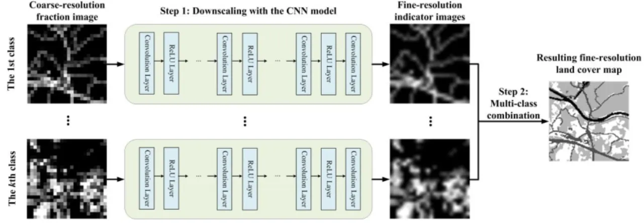
A two-step SRM algorithm (Ling et al. 2013) was used in this letter (Fig. 1). In the first step, for each land cover class, a fine spatial resolution indicator image is estimated by downscaling the coarse resolution fraction image with a convolutional neural network (CNN). In the second step, all of the fine spatial resolution indicator images are combined to generate a fine resolution multi-class land cover map.

2.2 The CNN downscaling model

The objective of the first step of the SRM analysis is downscaling the coarse resolution fraction image to a fine spatial resolution indicator image, in which the pixel’s value is taken to represent the possibility that the fine resolution pixel belongs to a specified land cover class. Here, the network structure of a very deep CNN (Kim, Lee, and Lee 2016) was used for the downscaling. The CNN used comprised 20 layers. The image input layer was followed by the first 2-D convolutional layer that contained 64 filters of size 3×3 and a rectified linear unit layer. The second to the penultimate layers of the CNN were 18 alternating convolutional and rectified linear unit layers. Every convolutional layer contained 64 filters of size 3×3×64, where a filter operated on a 3×3 pixels region across 64 channels. The last layer of the CNN model consisted of a single filter of size 3×3×64.

The CNN model was trained to learn the relationships for the downscaling with a set of training samples. Each training sample consisted of a pair of images that were small extracts taken from the data: a coarse resolution image and its corresponding fine resolution image. These training images had a fixed size that was determined by the structure of the CNN model used, and were often extracted from images simulated from fine resolution land cover maps. The latter depicted K classes and was used to generate K

fine resolution indicator images, one for each land cover class. If the area represented by a pixel belongs to the kth class, the value of this pixel is set to be 1 for the kth indicator image, and 0 for other indicator images. A coarse resolution fraction image for each land

cover class was simulated by spatially degrading the fine resolution indicator images according to the selected zoom factor.

Simulated training samples were used to train the CNN models, one for each land cover class. The simulated coarse resolution fraction image was interpolated to a fine resolution image. Here, the interpolation was achieved by a cubic convolution analysis. Taking the interpolated image as the input, the CNN model was then trained to predict the residual image that depicts the difference between the interpolated image and the actual fine resolution image (Kim, Lee, and Lee 2016).

Once trained, the CNN model was used to downscale the coarse resolution fraction image. The latter was first interpolated to a fine resolution image which was input to the trained CNN model to estimate a residual image. By adding the input interpolated image and the output residual image, a fine resolution indicator image was produced.

2.3 The multi-class combination model

The fine resolution indicator images generated for all land cover classes were combined to produce a fine resolution land cover map. Here, the maximal value rule, which aims to maximize the sum of indicator values of all fine resolution pixels in each coarse resolution pixel, was used to assign the pixel class labels in the fine resolution map.

In each coarse resolution pixel, the maximal value rule can be expressed as the following optimization problem:

Maximize 1 1 ( ) ( ) z z K k k v k E x v p v    



1 if fine pixel is a member of the land cover class ( ) 0 otherwise k v k x v    . (2) Subject to 1 ( ) 1 K k k x v  



1 ( ) z z k k v x v N   



value p v_k( ) for the kth class, and N_k is the number of fine resolution pixels of the kth

class calculated from the fraction images. A linear optimization model was used to find the solution, and a normalization procedure was applied on all fine resolution indicator images to address problems associated with small fractional values in neighbouring pixels (Ling et al. 2013).

3. Experiments

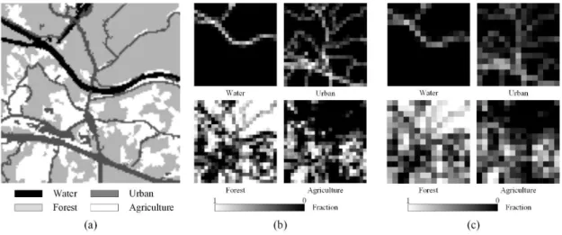
The proposed DeepSRM algorithm was assessed using a data set simulated from the National Land Cover Database 2001 (NLCD 2001), a raster based 16-class land cover map with spatial resolution of 30 m over all 50 states and Puerto Rico across the conterminous United States of America. A small region comprising 120×120 pixels was used with the original 16-class land cover scheme converted to one comprising four general land cover classes: water, urban, forest, and agriculture (Fig. 2a). Two zoom factors, z = 5 and z = 8, were used. At each zoom factor, synthetic coarse fraction images were simulated by averaging the fine resolution pixel values contained within each coarse pixel ( Fig. 2b and 2c).

Using simulated coarse resolution fraction images as input, the DeepSRM algorithm was used to estimate a fine resolution land cover map. To aid evaluation of the approach, a set of other popular mapping methods were also applied to the data: hard classification (HC), the pixel swapping SRM model (PS) (Atkinson 2005), the bilinear interpolation based SRM model (BI) (Ling et al. 2013), the back-projection neutral network based SRM model (BP) (Zhang et al. 2008) and the one step learning SRM model (OSL) (Ling et al. 2016). The accuracy of the fine resolution maps generated from these algorithms

was evaluated by comparing class labels of all pixels in the estimated land cover maps with those of the original fine resolution land cover map. Accuracy was expressed in terms of the percentage of correctly allocated cases or overall accuracy.

The training samples used in the CNN model of the proposed DeepSRM algorithm were generated from 200 subsets of NLCD land cover maps, each comprising an area of 400 × 400 pixels. The training parameters used by Kim et al. (2016) were adopted. Specifically, the mini-batch size was 64, the number of training epochs was 80, the initial learning rate was 0.1 and it was reduced by a factor of 10 every 20 epochs. The training time was approximately 9 hours for each land cover class; the work was undertaken using the Matlab platform running with a NVIDIA X1080 GPU.

4. Results and discussion

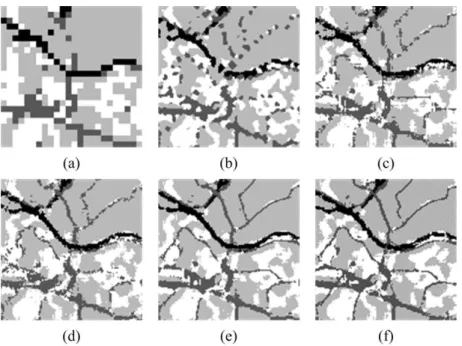
The land cover maps produced by the set of methods are shown in Fig. 3 and Fig. 4. The land cover maps produced by most SRM algorithms were visually superior to those produced by HC which had, as expected, unrealistic jagged boundaries. For all SRM algorithms, the fine resolution land cover maps produced by the algorithms based on the spatial dependence models, PS and BI, were inferior to those produced with the use of learning based algorithms such as BP, OSL, and DeepSRM. For example, with the output from the PS, many linear land cover features are wrongly grouped into round patches, while in the BI results, there were many irregular linear artifacts.

The advantage of the learning based SRM algorithms over the PS and BI arose mainly because they include in the analysis information on the spatial pattern of land cover obtained from the fine resolution land cover maps. The differences between the learning based methods related to the method used to model the relationship between coarse and fine resolution images. For example, the BP approach used a conventional shallow neural network and the OLS method adopted a linear weighted average approach,

while the very deep neural network in DeepSRM had greater ability to model complex non-linear relationships. As a result, the map produced by DeepSRM was superior to that produced by BP and OLS.

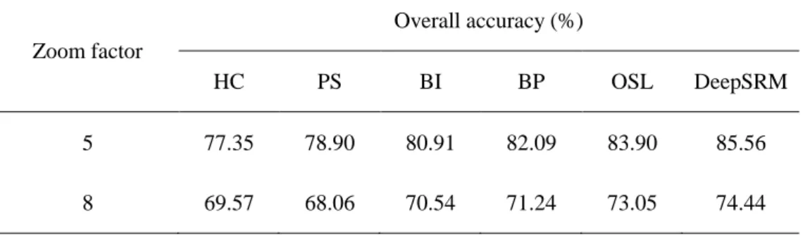
The accuracy of the land cover maps produced by the different methods at both zoom factors are shown in Table 1. At both zoom factors, land cover maps produced by HC, PS and BI were less accurate than those obtained from the learning-based methods of BP, OSL, and DeepSRM. These results highlight that the spatial pattern of land cover learned from the fine resolution land cover maps was superior to the simple representation obtained with the maximal spatial dependence model. Furthermore, the proposed DeepSRM algorithm was superior to the other two learning based SRM algorithms, BP and OSL, yielding the most accurate fine resolution land cover maps. For example, at the zoom factor of 5, the map from DeepSRM was 1.66% and 3.47% more accurate than the maps obtained from the OSL and BP methods respectively. The results highlight the potential of deep learning in a SRM analysis which may help remote sensing achieve more fully its potential as a source of land cover information.

5. Summary and conclusions

This letter proposed the DeepSRM algorithm that aims to use deep learning concepts in SRM. The proposed DeepSRM algorithm is a two-step method. The first step downscales input coarse spatial resolution fraction images to fine spatial resolution indicator images for all land cover classes. This is achieved by training a deep CNN model to represent the non-linear relationship between coarse and fine resolution images. Then, all estimated fine spatial resolution indicator images are combined to produce the resultant land cover map in the second step, by solving an optimization function which is constructed based on the maximal value principle. Experimental results showed that the proposed

DeepSRM algorithm outperformed state-of-the-art SRM algorithms in terms of the accuracy of the maps produced.

Although this letter only provides an initial result, it is believed that deep learning has the potential to further enhance SRM analysis. There are a range of issues that need to be addressed to fully exploit the approach. For example, fraction errors are a major challenge in real-world applications of SRM. The de-noising CNN model has the potential to address this problem, and can be integrated with the super-resolution CNN model. Additionally, it may be possible to refine the method to accommodate for relationships between the classes rather than simply downscaling for each class independently. There is also scope for further research on the CNN model used for image super-resolution and for usefully integrating other data that may be available, perhaps at different spatial and temporal scales, into the analysis.

Acknowledgment

This work was supported in part by the Strategic Priority Research Program of Chinese Academy of Sciences (Grant No. XDA2003030201). We are grateful to the editor and referees for their constructive comments on the original manuscript.

References

Atkinson, P. M. 2005. "Sub-pixel target mapping from soft-classified remotely sensed imagery." Photogrammetric Engineering and Remote Sensing 71 (7):839-846. doi: 10.14358/pers.71.7.839.

Atkinson, P.M. 2009. "Issues of uncertainty in super-resolution mapping and their implications for the design of an inter-comparison study." International Journal of Remote Sensing 30 (20):5293-5308. doi: 10.1080/01431160903131034.

Chen, Y.h., Y. Ge, Y. Chen, Y. Jin, and R. An. 2018. "Subpixel land cover mapping using multiscale spatial dependence." IEEE Transactions on Geoscience and Remote Sensing 56 (9):5097-5106. doi: 10.1109/tgrs.2018.2808410.

Dong, C., C. C. Loy, K. He, and X. Tang. 2016. "Image super-resolution using deep convolutional networks." IEEE Transactions on Pattern Analysis and Machine Intelligence 38 (2):295-307. doi: 10.1109/TPAMI.2015.2439281.

Foody, G. M. 2002. "The role of soft classification techniques in the refinement of estimates of ground control point location." Photogrammetric Engineering and Remote Sensing 68 (9):897-903.

Foody, G. M., A. M. Muslim, and P. M. Atkinson. 2005. "Super-resolution mapping of the waterline from remotely sensed data." International Journal of Remote Sensing 26 (24):5381-5392. doi: 10.1080/01431160500213292.

Ge, Y., S. Li, and V.C. Lakhan, 2009. "Development and testing of a subpixel mapping algorithm." IEEE Trans. Geosci. Remote Sens. 47: 2155-2164. doi: 10.1109/tgrs.2008.2010863.

Ge, Y., Y. H. Chen, S. P. Li, and Y. Jiang. 2014. "Vectorial boundary-based sub-pixel mapping method for remote-sensing imagery." International Journal of Remote Sensing 35 (5):1756-1768. doi: 10.1080/01431161.2014.882034.

Kim, J., J. K. Lee, and K. M. Lee. 2016. "Accurate image super-resolution using very deep convolutional networks." In IEEE Conference on Computer Vision and Pattern Recognition, 1646-1654. doi: 10.1109/cvpr.2016.182.

Ling, F., Y. Du, X. D. Li, W. B. Li, F. Xiao, and Y. H. Zhang. 2013. "Interpolation-based super-resolution land cover mapping." Remote Sensing Letters 4 (7):629-638. doi: 10.1080/2150704x.2013.781284.

Ling, F., Y. Du, X. D. Li, Y. H. Zhang, F. Xiao, S. M. Fang, and W. B. Li. 2014. "Superresolution land cover mapping with multiscale information by fusing local smoothness prior and downscaled coarse fractions." IEEE Transactions on

Geoscience and Remote Sensing 52 (9):5677-5692. doi:

10.1109/tgrs.2013.2291902.

Ling, F., Y. Du, F. Xiao, H.P. Xue, and S.J. Wu. 2010. "Super-resolution land-cover mapping using multiple sub-pixel shifted remotely sensed images." International

Journal of Remote Sensing 31 (19):5023-5040. doi:

10.1080/01431160903252350.

Ling, F., X. D. Li, F. Xiao, and Y. Du. 2014. "Superresolution land cover mapping using spatial regularization." IEEE Transactions on Geoscience and Remote Sensing

52 (7):4424-4439. doi: 10.1109/TGRS.2013.2281992.

Ling, F., Y. H. Zhang, G. M. Foody, X. D. Li, X. H. Zhang, S. M. Fang, W. B. Li, and Y. Du. 2016. "Learning-based superresolution land cover mapping." IEEE Transactions on Geoscience and Remote Sensing 54 (7):3794-3810. doi: 10.1109/tgrs.2016.2527841.

Mertens, K. C., B. De Baets, L. P. C. Verbeke, and R. R. De Wulf. 2006. "A sub-pixel mapping algorithm based on sub-pixel/pixel spatial attraction models."

International Journal of Remote Sensing 27 (15):3293-3310. doi: 10.1080/01431160500497127.

Muad, A.M., and G.M. Foody, 2012. "Impact of land cover patch size on the accuracy of patch area representation in HNN-based super resolution mapping." IEEE Journal of Selected Topics in Applied Earth Observations and Remote Sensing 5(5):1418-1427. doi:10.1109/jstars.2012.2191145.

Zhang, L. P. , K. Wu, Y. F. Zhong, and P. X. Li. 2008. "A new sub-pixel mapping algorithm based on a BP neural network with an observation model."

Neurocomputing 71 (10-12):2046-2054. doi: 10.1016/j.neucom.2007.08.033. Zhang, L., L. Zhang, and B. Du. 2016. "Deep learning for remote sensing data: A

technical tutorial on the state of the art." IEEE Geoscience and Remote Sensing Magazine 4 (2):22-40. doi: 10.1109/MGRS.2016.2540798.

Zhang, Y. H., Y. Du, F. Ling, S. M. Fang, and X. D. Li. 2014. "Example-based super-resolution land cover mapping using support vector regression." IEEE Journal of Selected Topics in Applied Earth Observations and Remote Sensing 7 (4):1271-1283. doi: 10.1109/jstars.2014.2305652.

Table 1. Overall accuracy of land cover maps produced by different methods. Zoom factor Overall accuracy (%) HC PS BI BP OSL DeepSRM 5 77.35 78.90 80.91 82.09 83.90 85.56 8 69.57 68.06 70.54 71.24 73.05 74.44

Figure 1. The flowchart of the proposed deep learning based super-resolution mapping model.

Figure 2. Dataset used in the experiment. (a) is the reference fine resolution land cover map with four classes (120 pixels × 120 pixels); (b) coarse resolution fraction images simulated for the fine resolution land cover map in (a) with zoom factor z=5, and (c) coarse resolution fraction images simulated for the fine resolution land cover map in (a) with zoom factor z=8.

Figure 3. Land cover maps produced by different methods at the zoom factor z=5. (a) HC, (b) PS, (c) BI, (d) BP, (e) OSL, (f) DeepSRM. Refer to Figure 2 for land cover

class legend.

Figure 4. Land cover maps produced by different methods at the zoom factor z=8. (a) HC, (b) PS, (c) BI, (d) BP, (e) OSL, (f) DeepSRM. Refer to Figure 2 for land cover