SERC DISCUSSION PAPER 160
First-Come First-Served:
Identifying the Demand
Effect
of Immigration Inflows on
H
ouse Prices
Rosa Sanchis-Guarner (SERC & Grantham Institute)
This work is part of the research programme of the independent UK Spatial Economics Research Centre funded by a grant from the Economic and Social Research Council (ESRC), Department for Business, Innovation & Skills (BIS) and the Welsh Government. The support of the funders is acknowledged. The views expressed are those of the authors and do not represent the views of the funders.
First-Come First-Served: Identifying the Demand Effect
of Immigration
Inflows on
House Prices
Rosa Sanchis-Guarner*
May 2014
* Spatial Economics Research Centre & The Grantham Research Institute on Climate Change and the Environment, London School of Economics
Abstract
An inflow of immigrants into a region affects house prices in three ways. In the short run, housing demand increases due to the increase in foreign-born population. In the long run, immigrants affect native location decisions and housing supply conditions. Previous research on the effect of immigration on local house prices has argued that the impact of immigrant demand cannot be separated from the demand changes due to native relocation or that the impact of immigrants on native mobility has no consequences on the estimates. In this paper I propose a methodology to pin down the immigrant demand effect. I apply it to Spanish data during the period 2002-2010 and I show that overlooking the impact of immigration on native mobility induces a sizeable bias in the short-run estimates. My results are robust to controlling for changes in housing supply.
Keywords:Immigration, housing markets, instrumental variables
1
Introduction
The study of the local economic impact of immigration has been a very active area of re-search in the last 20 years. Large immigration inflows impact the spatial distribution of pop-ulation within a country. The location choices of the foreign-born directly change the com-position and size of the population residing in a given area. An inflow of immigrants directly increases the population of a region. Immigrants also influence the location decisions of nat-ives, indirectly changing the population size of different locations. Changes in population affect the labour force of an area, and therefore impact not only average wages and employ-ment rates, but also their distribution. Changes in the labour market conditions will, as a result, affect other economic aspects such as productivity, skills composition, and ultimately growth and welfare. Not only do immigrants affect the production factors, they also con-sume amenities and housing services in the places to which they locate and thus influence the spatial equilibrium. As a consequence, the study of the local effects of immigration on housing markets is central to urban economics.
Most of the theoretical and empirical contributions on the study of the impact of immig-ration in receiving regions have originated from the analysis of their labour market effects1. Recently, research has focused on the impact of immigration on a richer set of economic and social outcomes like productivity, crime or consumption (see Ottaviano & Peri, 2013;
Nathan,2013, for recent reviews). A small number of papers have provided evidence on the effect of immigration on (consumption) goods prices (Lach,2007;Cort´es,2008;Zachariadis,
2011). They have mostly found negative effects of an increase of low-skilled immigration on (generally immigrant-labour intensive) goods prices. For a given supply, following an increased in foreign-born population, intensified spatial competition on the consumption of goods, amenities and housing services may push prices up in the short run. In the long run, the sign and size of the impacts does not only depend on the response of the supply of goods but also on any induced relocation of natives following the immigrant inflows. The net effect on prices would therefore be the result of total changes in the demand side (from immigrant and natives) and of changes in the supply side. These supply-demand mechan-isms operate in the analysis of the effects of immigration on house prices. Previous evidence for the US (for exampleSaiz,2003,2007;Ottaviano & Peri,2011) has generally found positive (long-run) impacts of immigration on both rents and prices2.
There are two major challenges when estimating the causal effect of immigration inflows on local house prices. The first one relates to the fact that immigrant location choices and house price dynamics might be driven by the same underlying unobserved factors. An es-timate of the impact of immigrant inflows on average house prices that fails to take this into account will be biased. For example, if immigrants locate in areas where prices are growing slower, coefficients obtained using OLS estimation techniques would be too small. This issue is generally addressed in the literature using instrumental variables, panel data estimates and control variables. The second challenge relates to the interpretation of the es-timates. As noted bySaiz(2007), in the long run we need to take into account not only the
1Hanson(2008),Dustmann et al.(2008),Longhi et al.(2009),Pekkala-Kerr & Kerr(2011) andNathan(2013)
provide recent reviews of the literature.
2Other studies areGreulich et al.(2004), which assesses the impact of immigrant on native renter
house-holds housing consumption opportunities;Stillman & Mar´e(2008), which provide estimates for New Zealand andNathan(2011) which provides estimates for the UK.
impact of immigrants on housing demand but also the changes that immigration inflows in-duce on housing supply, density of housing and native mobility. A well-identified long-run reduced-form estimate is a combination of all these effects. However, the interpretation of the underlying channels is unclear.
The current paper addresses both issues. First, I estimate the long-run effect of immig-ration inflows on average local house prices using a first differences and instrumental vari-ables (IV) approach, adding a large set of area trends and controls. In order to obtain un-biased causal estimates, I construct an improved shift-share instrument that combines his-torical immigrant location patterns with predicted national inflow by country of origin ob-tained from a push-factors gravity model (full details are given in Sections 2.3 and A.2). Next, I propose a methodology to identify the short-run effect of immigration: their direct demand impact on local prices. With this strategy, the estimated coefficient isolates the ef-fect of the increase in the immigrant demand on prices from the efef-fect of immigrations on housing supply and native mobility. This enables a clearer economic interpretation of the estimates. This latter issue has drawn little attention in the literature, where the effect of immigrants on housing supply or native mobility has been studied separately.
The proposed strategy is applied to investigate the impact of the large immigration inflows on house prices using Spanish data. Between 2001 and 2010 both the number of foreign-born residing in Spain and house prices significantly increased, providing a suitable setup to gain further insights on the impact of immigrations on prices. Motivated by the sub-stantial size of the immigration inflows, a number of recent empirical works have analysed the impact of immigration in Spain on various economic outcomes. Most of the papers have focused on the labour market impacts (Bentolila et al.,2008;Carrasco et al.,2008;Gonz´alez & Ortega,2010;Amuedo-Dorantes & de la Rica,2011;Amuedo-Dorantes & Rica,2013), but a number of contributions have studied other aspects like the effect of immigration on output mix (Requena et al., 2009), trade (Peri & Requena, 2010), productivity (Kangasniemi et al.,
2009), or even crime (Alonso-Borrego et al.,2011).
A handful of recent works have also provided some evidence of the impact of immigra-tion on house prices in Spain.Talavull de la Paz(2003) explores their different determinants using a sample of Spanish cities during the period 1989 to 1999. She investigates the role of population and economic activity specialisation as explanatory variables of city price dif-ferentials. She finds that population is strongly significant in explaining house price levels while economic structure does not appear to have any significant effect on house prices.
Sosvilla-Rivero(2008) analyses the effect of immigration during the period 1995-2007 using regional data and assesses the over-valuation of the house prices with respect to economic fundamentals. He finds that almost half of the over-valuation can be attributed to immigra-tion flows, which he interprets as a positive relaimmigra-tionship between immigraimmigra-tion and prices.
Garc´ıa-Montalvo (2010) explores the role of land regulation and immigration on Spanish municipalities during the period 2001 to 2005 but, conversely to the other studies, he finds no effect of immigration inflows using a long-differences IV estimation. Finally, Gonz´alez & Ortega (2013) investigate the impact of immigrant inflows on sale prices and housing construction during the Spanish recent house-boom period. They find substantial positive causal effects of immigration inflows on both outcomes. Their paper is the closest to the present one, but the period of analysis, empirical strategy and research aim is different.
Building upon these contributions, the present paper estimates both the short-run (de-mand driven) and the long-run (after supply and mobility adjustments) impact of
immig-ration on local house prices. I estimate this impact both on sale and rental prices. To obtain the coefficients I exploit a panel dataset for Spanish provinces (NUTS3) for the period 2001-2010. This period of analysis covers a subperiod of high boom (2001-2008) and bust of the housing markets (2008-2010), which provides sufficient variation in the data to adopt a very demanding empirical strategy.
Most existing papers (Saiz,2007;Cort´es,2008;Gonz´alez & Ortega,2013) rely on the exist-ing US evidence3to argue that native area displacement due to immigration is small or not large enough to cancel increased demand stemming from increased area population. Even if natives were displaced by immigrant inflows, the reduction in native demand would be smaller than the increase in foreign-born demand and therefore area demand would in-crease. Finding a positive (long-run) impact of immigration on local house prices is gen-erally interpreted as supportive of no or little native displacement. If the effect on native mobility is small enough, the short-run and the long-run estimate would be of very similar magnitude. Thus, these papers make no distinction between short and long-run adjustments when interpreting their results.
In this paper, I first obtain the impact of immigration inflows on prices by estimating a specification and strategy similar toSaiz(2007). I regress the annual local house price growth on an immigration ratio, which is defined as the total immigrant inflow normalised by the beginning-of-the-year area population. To obtain unbiased causal parameters, I use a shift-share instrument. The estimated elasticities are 1.1% for rental prices and between 2.2 and 3% for sale prices. These coefficients correspond to the long-run effect. I then explicitly test the impact of immigrant inflows on native mobility and, consistently with existing estimates for Spain (Fern´andez-Huertas et al.,2009), I find that immigrants attract natives to areas in which they locate (approximately 6 natives for each 10 foreign-born). Given this finding, I argue that ignoring this effect induces a sizeable bias in the short-run estimates. To identify the impact that is only due to increased immigrant housing demand, I re-estimate the coeffi-cient using solely the variation on population growth which is due to exogenous location of foreign-born. The estimated elasticities using my proposed methodology are 0.7% for rental prices and between 1.4 and 2.1% for sale prices. This implies that the long-run estimates are up to 60% larger when we ignore the relationship between immigration and native location decisions. I furthermore explore the impact that changes in housing supply have on the es-timates and I find that they have very little effect on the coefficients. These results are robust across specifications, to different data sources and to the use of different definitions of the instrument.
By providing a strategy to separate the long and short-run immigration impact, the main contribution of this paper is methodological. My results add to the evidence on the area effects of the recent immigrant wave in Spain. Contrary to existing estimates, I isolate the effect due to direct increases in immigrant local house demand from long-run adjustments affected by changes in local housing supply and native spatial relocation. I also obtain the long-run estimate. The comparison of both coefficients informs us about the role of direct (foreign-born) and indirect (native) demand on increasing local house prices, and on the role of housing construction on mitigating price increases. Finally, I add to previous evidence on the effect of immigration on Spanish housing market by estimating the effect not only for house sale prices but also on rental prices.
The rest of the paper is organised as follows. Section 2describes the empirical strategy: the empirical specification is explained in 2.1, the strategy to identify the effect of foreign-born demand in2.2and the identification strategy in2.3. Descriptive statistics are provided in2.4. Section3discusses the results and the robustness tests. Finally, Section4contains the conclusions and the discussion of the limitations of the analysis.
2
Methodology
2.1
Empirical specification
In order to estimate the causal effect of changes in foreign-born population on the growth of house prices, I use a linear empirical specification similar to Saiz(2007). The 50 Spanish provinces iare the geographical unit of observation, which are grouped into 17 regions r4.
t denotes time periods (years).∆log(hpri,t) is the change of the natural logarithm of house prices in province i during year t, FBin f lowi,t−1/populationi,t−1 is the immigration ratio
duringt−1,λt are time fixed effects,γr are regional fixed effects,Ziis a matrix of province time-invariant attributes and ∆Xi,t−2 is a matrix of province time-varying controls. Finally,
εi,t is the random shock. The empirical equation takes the form:
∆log(hpri,t) = β FBin f lowi,t−1
populationi,t−1
+φ0Zi+δ0∆Xi,t−2+λt+γr+εi,t (1) The independent variable of interest is the immigration ratio: it is defined as the inflow of immigrants into provinceiduring a given period divided by the population in the province initial population)5. The inflow of immigrants duringt−1 is calculated as the change in the foreign-born population between January t−1 and Januaryt . Population int−1 denotes the stock of total residents (natives and foreign-born) at the end of period t−2. Given the nature of housing services, the main specification uses the immigration ratio lagged one period with respect to the changes in prices6.
Using an immigration ratio instead of gross inflows as the measure of “immigration” has three advantages. Firstly, for a given housing stock, the changes in demand affecting house prices depend on the number of immigrants moving into the province (new demand) and on the demand from area residents (existing demand). If we aim to measure the impact of demand from immigrant arrivals, we need to take into account how large new demand is as compared to demand from existing residents. For a given size of the immigrant inflows, the impact of new arrivals on housing demand would be relatively smaller in more populated regions. This would lead to different house price growth dynamics than in less populated regions. Using the ratio over population we can take into account the “relative” size of the immigration inflow, which better captures the effect of immigration on housing demand. Secondly, by using the ratio we also eliminate any unobservables that might equally affect both the numerator (immigration inflow) and the denominator (original province’s popula-tion). As explained in Peri & Sparber (2011), and suggested by Card (2001), standardising
4Provinces correspond to the European NUTS3 and regions to NUTS2. I exclude the African territories due
to their historical particularities and the lack of reliable data.
5The Spanish administrative population data is dated on the 1stof January. Referring to the beginningt−1
is equivalent to referring to the end oft−2.
the immigration inflow by the size of the population allows us to eliminate the spurious correlation between higher inflows and higher price changes. This correlation could arise due to the fact that the average and standard deviation of both variables are likely to be proportional to the total population in the province. Finally, this setup allows us to interpret the coefficient βas an elasticity: a 1% increase in the ratio has a β% effect on the change in prices.
The first differences setting of equation (1) eliminates any unobservable province char-acteristics which might be correlated with the level of house prices and the level of foreign-born population in the province. Time fixed effectsλt control for common shocks affecting the growth of prices of all provinces in Spain in a given year (for example, a tax deduction on mortgage payments, a subsidy to renting or a better financial climate). There could still exist some unobserved factors at the area level which are correlated with the changes in house prices and the changes in foreign-born stocks (numerator of the immigration ratio). Not including these would bias the estimation ofβ. To tackle this issue, first I include region fixed effects γr and regional trends γr ∗t. These fixed effects control for time-invariant re-gional characteristics (or trends) which might affect the price growth and the immigration ratio and which are not common to the whole country. In the most demanding specification I include province fixed effects (γi). These control for unobservables at the province level which are correlated with changes in prices and in the immigration ratio. This specification corresponds to a first differences fixed effects estimation.
Vector Zi contains time-invariant province attributes. These variables control for the fact that provinces with different levels of the time-invariant characteristics might have different growth trends in the house prices levels and in the stocks of foreign-born population. Given that region fixed effects (γr) are also included, the province attributes control for differential growth trends of the provinces around their common regional trend. The vector includes a set of geographical (coast dummy, length of the coastline, surface of the national parks) and weather (average temperature and average rain precipitation in January) characteristics and beginning of the period amenities (number of restaurants and bars in 2000, number of retails shops in 2000, number of doctors in 2000 and a comparative index of the importance of the tourism sector in 2000).
In order to control for the role of housing supply in driving both house price dynamics and immigration inflows I add time-invariant province housing controls. I include the share of developable land in 2000 and a proxy for land regulation (the share of municipalities in the province which had land use plans in 1999). More developable land and regulation could directly affect the rate of construction in the province. Different construction dynamics could drive immigrants to the province as it provides working opportunities and more af-fordable housing. I also account for beginning-of-the-period housing market characteristics that could affect prices and immigrant inflows. These are the proportion of rented prop-erties and the proportion of empty dwellings, both in 2001. Provinces in which renting is more common can have different trends in the growth of supply and attract immigrants differently as these are more likely to rent7. Prices in provinces in which the proportion of unoccupied dwellings is larger could be growing at a slower rate because the supply of homes is effectively higher in these locations. When I use province fixed effects, I control for all time-invariant attributes, soZidrops.
7According to the 2007 National Immigration Survey (Encuesta Nacional de Inmigrantes 2007around 77% of
Vector ∆Xi,t−2 contains time-varying characteristics (in changes). However, if the
vari-ables included inXi,t−2are “bad” controls – variables that could well be outcome variables in
equation (1) (Angrist & Pischke,2009) –, their inclusion would not reduce the omitted vari-able bias. To mitigate the effect of bad controls, I use a lag with respect to the immigration ratio, so the variables are measured one year before the immigrants locate in the province. Hence, I use the changes in the variables during t−2, one period before the inflows (t−1) and two periods before the change in prices (t). I control for the growth in gross domestic output (GDP) and the changes in the unemployment rate. Richer provinces which are grow-ing faster and employgrow-ing more people could be attractgrow-ing more immigrants and thus could also have higher growth in house prices. I also control for changes on the number of credit establishments and on the share of saving banks because they could have affected the avail-ability of credit, which might have pushed sale house prices up by influencing housing tenure decisions (Cu ˜nat & Garicano,2010).
If we believed there is substantial time dependence on both the immigration ratio and on the growth of house prices8, lagging the controls one period with respect to the immigration ratio would not be enough to overcome the problem of bad controls. In this case, we would not be sure whether our control, for example GDP growth, was not directly determined by prospects of future changes in prices and immigration. Given that equation (1) controls for area and time fixed effects, the time-varying controls would only be eliminating the bias induced by annual changes in the province characteristics which are not captured by these fixed effects and which are affecting the change in prices and the change in immigration ratio at the same time. In other words, an annual shock in GDP in province which is not common to all provinces in Spain and which is different from the average growth in the period. These changes are likely to be small, so the reduction in the bias caused by the in-troduction of time-varying controls is likely to be small (which is the case, as explained in Section 3). The empirical results are very robust to the exclusion of∆Xi,t−2, and the
estim-ated β coefficient is very similar with and without time-varying controls. The main results are obtained including time-varying controls, but the qualitative conclusions would remain unaltered if we excluded them.
To carry out the empirical analysis I used data from several sources. Immigrant and population data comes from the Municipal Register (Padr´on Municipal), which keeps an annual record of all registered individuals in a municipality over time regardless of their legal immigration status. This is the most reliable source to study the impact of the size of immigration on area economic outcomes. House sale price data was obtained from Uriel-Jim´enez et al.(2009), who provide an improved version of the Housing Department9 Aver-age Province House Price Index. Data on rental prices was obtained combining data from the Housing Department and the National Institute of Statistics. Finally, data on the controls comes from several sources including the National Institute of Statistics, the Housing De-partment, the 2001 Census and theLa CaixaSpanish Economic Yearbook. Full details on the data sources is provided in SectionA.1in the Appendix. Table1provides summary statistics for these variables.
8The correlation between the immigration ratio and the lagged immigration ratio is 0.60, between
changes/lagged changes in sale prices is 0.76 and changes/lagged changes in rental prices 0.50.
2.2
Identifying the impact of immigrant demand on prices
Foreign-born population inflows, by increasing local population (Card, 2007), have a pos-itive impact on the growth of house prices in the short run, due to increased demand. The economic intuition behind this is a simple demand-supply result. For a given level of popu-lation in a region, after a large immigration inflow, increased competition in housing markets forces both newly arrived immigrants and stayers to bid higher to buy or rent a property. For a given supply, a positive immigration inflow into a region could be translated into an increase in demand of housing services, thus pushing up house prices.
This is the intuition behind the model developed inSaiz(2007). An increases in foreign-born population in a given location raises total population and then pushes demand and prices in the short run. In the long run, we also need to take into account the effect of the changes on housing supply (construction), on housing consumption (density) and on the mobility of natives or previous residents (displacement) on prices. These three channels can be affected by immigration. Unless we directly control for these, an estimate of βin equa-tion (1) would capture the combination of all these mechanisms. The use of instrumental variables and controls yields unbiased estimates of the long-run coefficient. In this section I propose a method to isolate the immigrant demand effect (short-run) from the long-run effect. To do this, we need to consider the three long-run adjustment mechanisms: housing density, housing stock and native mobility. I discuss each of these channels in detail below.
The first one is housing density. Table 2 displays the total population and the number of residential dwellings in the 50 provinces of study for every year between 2001 and 2010. The table shows the ratio of total (private) housing stock over total population10. Housing density remained relatively stable during the period. Even if we cannot draw definitive con-clusions, mainly due to the lack of reliable yearly data on housing vacancies, these numbers suggest that, if anything, intensive construction together with large immigrant inflows kept the ratio of houses/population relatively constant (or even increased it)11. Directly including changes in house density in the regressions is problematic as both population and housing stocks are endogenous to house prices, given how little it changed over the period of ana-lysis, it is unlikely that differences in housing density substantially affected house prices in the long run.
Table2also shows that a large number of new housing units were constructed between 2001 and 2010, almost 5 million (4.45 million if we take into account empty properties). We would expect that increased supply would, at least partially, mitigate the rise in prices caused by the increase in demand. House construction could also be correlated with immig-ration inflows if immigrants locate in areas where house construction is higher (due to job opportunities or more availability of housing). I account for the effect of housing supply on house prices in two ways. Firstly, in the estimation of (1) I include time-invariant province characteristics related to housing supply (geographical and housing market characteristics). As the model is estimated in first differences, these variables control for differential trends correlated to both immigration inflow and house price changes. Including time-varying sup-ply changes in the estimation of equation (1) as an additional control is very problematic,
10Private housing in Spain represents around 90% of the total stock.
11I used empty dwelling data to recalculate the ratio in 2001 and 2011 using only occupied properties. Doing
this, the ratio only increased 3 percentage points during the period (from 0.44 to 0.47), which is less than 0.3% per year.
because even if lagged, housing construction is a “bad” control given that construction is directly affected by immigration12. In Section 3.4, I include time-varying housing supply (log changes in the stock of residential dwellings) as an additional control and deal with the bad control problem using an IV strategy. When I control for housing supply, β does not capture the effect of immigration inflows on housing construction and thus the estimated coefficient is closer to the short-run immigrant demand effect.
The long-run effect of immigration inflows on any local economic outcomes also depends on what the literature has called “native displacement”13. Any estimated area effect of an inflow of immigrants would be the net result of changes in labour supply which stems from the foreign-born inflows plus any changes from natives relocation. The existence of native displacement has been used as an explanation for the lack of robust estimates of the impact of immigration on wages across US labour markets. The relocation of population across regions within a country would hinder the identification of any area-level effects, as the effects would dissipate throughout the country.
Numerous papers have investigated the relationship between immigration and natives displacement14. Most of them assume that immigrants displace natives from the regions they settle in (Card, 2001). However, as noted byOttaviano & Peri (2013), this assumption relies on immigrants and natives being homogenous in labour market characteristics. Im-migrants and natives of similar characteristics (for example low-skilled) would be compet-ing for the same (low-paid) jobs, thus we can expect immigrants to have some displacement effects on natives within narrowly defined labour market. In contrast, recent papers (Peri & Sparber,2009; Manacorda et al., 2012;Peri,2012; Ottaviano et al.,2013) show that, if native and immigrants are imperfect substitutes and specialise in different tasks, immigrants can promote efficient task specialisation and have a productivity-enhancing effect, increasing native wages.
In a recent article,Peri & Sparber(2011) review the existing evidence of native displace-ment in the US and, using simulated data, they assess the relevance of the tests which have been previously performed in the literature. They conclude that, based on the existing meth-ods, there is no robust evidence in favour of the existence of native displacement in the US. The authors suggest to test the native displacement hypothesis using a variation of the test proposed byCard(2007)15. We can use a “native ratio” in the left-hand-side of a specification similar to (1) and estimate:
natives in f lowi,t
populationi,t
=α FBin f lowi,t
populationi,t
+γt+γr+φ0Zi+δ0∆Xi,t−1+εi,t (2) where the variables in the right-hand-side denote the same elements as in equation (1). The sign and size of α captures the relationship between immigration inflows and native
loca-12In particular, Gonz´alez & Ortega(2013) find that immigrants have a positive causal impact on housing
construction.
13This issue gained renewed interest after the publication ofBorjas (2003). This paper criticized regional
immigration studies of the labour market impacts of foreign-born inflows, claiming that the United States (US) works as a single labour market and that the existence of displacement hampers the estimation of regional effects.
14For exampleCard & DiNardo(2000),Card(2001),Hatton & Tani(2005),Borjas(2006),Card(2007),Cort´es
(2008) andMocetti & Porello(2010).
15Card’s specification uses population growth as the left-hand-side variable, which includes both natives
tion. If the estimated α is negative this would indicate that natives are leaving the regions where the immigrants locate: displacement would be complete ifα = −1 or less than pro-portional if−1<α <016.
As in the case of labour markets, native mobility affects the estimation of the effect of immigration on local house prices. For a given population and housing stock in the area, immigration inflows would increase prices through increased housing demand in the short run. In the long run, native location decisions could be affected by the foreign-born inflows. Total housing demand would changes as consequence of total population changes, induced by immigrant and native spatial mobility. Thus, total changes in housing demand in the long run depend on how and if the natives relocate spatially after or at the same time as the immigrants arrive.
Previous authors have assumed that immigrants would displace natives in the housing markets in which they locate (Saiz,2007;Gonz´alez & Ortega,2013). As in the labour market case, this assumes that immigrant and natives are perfect substitutes. If native and immig-rants compete for the same type of housing or jobs or natives dislike immigimmig-rants, an inflow of immigrants could displace natives from a given housing market. If immigrants are het-erogeneous and complementary to natives they might mitigate the displacement effect or even co-locate in the same regions as natives. Some possible explanations are that immig-rants specialise in different tasks than natives (Ottaviano & Peri,2008;Ottaviano et al.,2013), so they do not compete for the same jobs, or that they consume different goods (Mazzolari & Neumark, 2011). Natives could co-locate with immigrants (α > 0) if these are attractive to them because they provide cheaper labour-intense goods (as suggested byCort´es, 2008) or because they generate positive externalities on natives wages or rents (Ottaviano & Peri,
2006,2007).
In his study of the effect of immigration on American rents, Saiz (2007) claims that if native outflows completely off-set immigration inflows, we would expect the increase in housing demand by immigrants to be completely balanced out by a decrease of housing demand from natives. The total (long-run) effect, and parameter β in equation (1), would be zero. If natives leave the area in greater numbers than immigrants enter, β would be negative because it would mean total housing demand (for a given supply) is decreasing. He suggests that finding a positive local effect of immigration in rents allows us to reject the complete native displacement in the labour market. Thus, the long-run coefficient provides indirect evidence of the relationship between immigrant inflows and native location.
As the aim of my paper is to estimate demand effect of immigration on prices, I dir-ectly estimate the effect of immigration inflows on native location decisions. If no causal relationship exists between immigration and native location, we can be quite certain that, conditional on supply, coefficientβin equation (1) is only capturing the effect (increased de-mand from) immigration on prices. In this case, the short and long-run impact would be the same, conditional on changes in housing supply. However, if a sizeable causal relationship exists, we need to be more cautious about the interpretation of the results17. In section3.2,
16As before, the native or foreign-born inflow is defined as the change in numbers duringtwhile population
intrefers to the stock at the beginning of the year (January).
17In their report, Fern´andez-Huertas et al. (2009) provide some non-causal evidence on the relationship
between immigration and native location. They find positive correlations although they claim that the size is negligible and cannot have any considerable impact on the estimation of local effects of immigration.Gonz´alez & Ortega(2013) also argue that native displacement would have no impact on the area level estimates. My results in Section3.2suggest differently.
I estimate the displacement hypothesis with Spanish data. I find substantial causal positive co-location of immigrants and natives. In section3.3, I propose a methodology to pin down the immigration demand effect of immigration on prices (short-run effect). I estimate the ef-fects using solely the variation on population growth which is due to exogenous location of foreign-born. I construct an instrument to predict the location of immigrants based on past ethnic networks. This is explained in the following section.
2.3
Instrumental variables strategy
As detailed in Section 2.1, the first step to achieve correct identification of the effects of immigration on prices is to include area fixed effects. These control for time-invariant unob-servables at the region or province level correlated at the same time with the immigration ratio and the growth in prices. When we include province dummies, the fixed effect es-timator exploits the variation in price changes and immigration inflows within provinces across time around the average changes during the period 2001-2010 (net of common na-tional shocks as time dummies are included). We need a substantial amount of variation to be able to identify the βparameter precisely. Because our period of analysis covers both a period of high growth (2001-2007) and of economic crisis (2008-2010), there is a fair amount of variation in the data to be able to identify the parameter of interests using a demand-ing empirical specification (first differences and includdemand-ing year and area fixed effects and trends).
Nevertheless, even after including area dummies and trends, consistent estimation of β still requires the regressor of interest to be uncorrelated with the time-varying part of the error term (local time-varying shocks affecting price growth and immigrant location at the same time). If this is not the case, we would still be finding inconsistent estimates of the coefficient of interest. There is no prior on the direction of the bias. The estimated β would be upward biased if immigrants are going to provinces with positive shocks or unobserved better economic prospects, while it would be downward biased if, for some reason, immigrants locate in province in which prices are growing slower.
In order to infer causality on the relationship between immigration and house prices growth, I estimate equation (1) using an IV approach. I construct the instrument adopting the “shift-share” methodology, which has extensively been used before, for instance byCard
(2001), Ottaviano & Peri (2006) or Peri(2009). Intuitively, the instrument is constructed by distributing year-to-year national variation of the variable of interest, –the “shift”–, using some rule, –the “share”–, to allocate this magnitude over space. In order to be a good instru-ment, both elements involved in the construction predicted regional yearly inflow must be orthogonal to local shocks related to the outcome variable, conditional on controls.
The most common immigration shift-share instrument exploits the fact that, to take ad-vantage of social and economic established networks, immigrants tend to disproportion-ately locate in areas where immigrants from the same nationality or ethnicity have located before. To predict current location patterns, I use historical location patterns to construct the “share” rule. For the national yearly immigration inflow, I use different approaches (details below). By combining these, I compute predicted local immigrant inflows which are used to construct an IV for the immigration ratio.
The immigration ratio in equation (1) is defined as the immigration inflow duringt−1 divided by total population (foreign-born plus natives) at the beginning oft−1. Denoting
foreign-born population asFBstockwe can express the immigration ratio for provinceias: FBin f lowi,t−1 populationi,t−1 = FBstocki,t−FBstocki,t−1 FBstocki,t−1+nativesi,t−1 = FBin f lowi,t−1 FBstocki,t−1+nativesi,t−1 (3) I construct the instrument followingPeri(2009). I predict the stock of foreign-bornFBstocki,t−1
by year and nationality, and I use this prediction to calculate the immigration inflow of the numerator (calculated as change in the stock) and I also use it in denominator as part of total population.
To impute the yearly immigrant population in each province by nationality of origin, I first calculate, for each province and each nationality, the share of immigrants (over the total number in Spain) that were located in that province in the base year. I denote provinces with
r18, time periods witht, nationalities or ethnic groups withn(N being the total number of nationalities). The base year used as the reference year of “past” location patterns is 1991. A list of the nationalities used (119 groups) appears in TableA.1. It is defined as:
shareni,1991 = FBstock n i,1991 ∑R r FBstocknr,1991 = FBstock n i,1991 FBstocknSpain,1991 (4)
This share is the proportion of immigrants located in a particular province i over the total immigrants from the same nationality located in Spain in 1991.
To obtain yearly predictions of the number of immigrants by nationality n, I multiply expression (4) by the current national stock of immigrants of nationality n. This stock is calculated summing the number of foreign-born of that nationality in all provinces in Spain except i, in year t. I exclude provincei from the summation to avoid using the stock I am trying to instrument for in the construction of the prediction of foreign-born. This stock is province-specific because for each provinceiwe exclude its own immigrant stock:
FBstocknSpain i,t =
∑
Rr6=iFBstocknr,t (5) The imputed foreign-born stock of a specific nationality nin province iat time tis thus calculated allocating yearly total national stocks (5) weighted by its historical share (4):imp FBstockni,t =FBstockSpain in ,t∗sharein,1991 (6)
To calculate the imputed total (all nationalities) foreign-born stock in province iat time
t, I sum (6) across nationalities:
imp FBstocki,t =
∑
N n imp FBstock n i,t (7) I use the change of the imputed total foreign-born population to calculate the imputed total inflow of immigrants (recall that population data is dated 1stJanuary). In order to ob-tain the first instrument for the immigration ratio as defined in expression (3), this imputed inflow is divided by the imputed population (imputed foreign-born plus native stock) inprovinceiat the beginning of the periodt−1. The instrument is constructed as follows:
IV1 imm ratioi,t−1=
(imp FBstocki,t−imp FBstocki,t−1)
imp FBstocki,t−1+nativesi,t−1
= imp FBin f lowi,t−1
imp populationi,t−1
(8) For this instrument to be valid it has to be sufficiently correlated with the immigration ratio but uncorrelated with the local shocks that affect house price variations, conditional on the controls and area and time fixed effects. The relevance of the instrument can be assessed by the value of the F-statistics of the instrument in the first stage of the 2-stage-least-squares (2SLS) regressions, and additionally by using under-identification and weak identification tests.
The exogeneity of the instrument depends on several conditions. Given the way the pre-dicted foreign-born stock (6) is constructed, we need that19:
1. The unobserved factors determining the location of immigrants in one province with respect to another in the base year (1991) is uncorrelated with the relative economic prospects of the two provinces during the period of analysis (2001-2010). In other words, immigrants in 1991 did not locate in Spain in the prospects of future relative growth during the 2001-2010 decade.
2. The only channel through which foreign-born geographical distribution in 1991 (second term in6) affects current changes in house prices is through its influence on shaping the current immigrants location patterns, conditional on controls (exclusion restriction). 3. The total (national) flow of immigrants in a given year (first term in6) has to be
exo-genous to specific province unobservable local shocks.
The choice of the base year determines the validity of conditions (1) and (2) but also the strength of the instrument. If the base year is very close to t, the instrument would be strong but its exogeneity can be questionable. If the base year is very far from t, it is more likely that the instrument is exogenous, but it may not be strong enough. The instrument is computed using data for the 1991 Census (foreign-born by country of nationality). In 1991 there was a sufficient stock of foreign-born in each province from each nationality to assure that our instrument is strong. Conditions (1) and (2) require that, conditional on controls, location choices in the base year are not driven by factors correlated to current changes in house prices (Saiz, 2007). These conditions are quite likely to be valid given that between 1991 and 2001 there was an important economic crisis (1992-1993) followed by economic recovery and growth (from 1997). It is unlikely that 1991 immigrants were able to predict these future shocks (or any other shock not captured in the province nor in the time fixed effects) ten years before our period of analysis starts.
The validity of condition (3) depends on the way the current national stock of immig-rants of nationality n is constructed. First, to avoid using the inflow for that we want to instrument for in our prediction (just scaled by sharein,base), term (5) is defined as the total inflow of immigrants from nationality ncoming to Spain at time tminus the inflow of im-migrants from nationalityncoming to provinceiat timet. Yet, we still require this term to be orthogonal to current local shocks. This assumption may be violated if location in provinces other than i is correlated with unobservable economic conditions of province i at a given
point in time t. This is probable, specially if our spatial units are small and the economic conditions that attract immigrants are spatially correlated. For example, the economic con-dition in “economically big” provinces (like Madrid or Barcelona) could influence the total number of immigrants deciding to come to Spain, even if they end up locating somewhere else (based on their ethnic networks).
To solve this issue, a similar strategy toSaiz(2007) andOrtega & Peri(2009) is adopted. I compute the yearly predicted total stock and inflow by country of origin from the results of a gravity model which depends only on push factors. These predictions replace term (5) in equation (6). Details of this procedure are given in the Appendix (sectionA.2.1). Using the predictions from estimating equation (A.1) in (A.2) to obtain (A.3), I redefine the instrument as:
IV2 imm ratioi,t−1 =
imp pred FBin f lowi,t−1
imp pred FBstocki,t−1+nativesi,t−1
(9) However, there could still exist a final issue with the construction of (9) which might make the instrument invalid. Total population stock, which appears in the denominator, is the result of the sum of the foreign-born (imputed prediction) plus the natives. As discussed in Section 2.2, the number of total natives residing in a given province might depend on the number of foreign-born in the same location or on unobservables correlated with house price growth. For this reason, I use a similar shift-share strategy to compute a prediction for the location of nativesimp nativesi,t−1, based on past location patterns. Details are given in
the Appendix (sectionA.2.2). Replacing the actual native stock by its prediction in equation (9), I finally define the main instrument as:
IVmain imm ratioi,t−1 =
imp pred FBin f lowi,t−1
imp pred FBstocki,t−1+imp nativesi,t−1
(10) I use IVmain ratioi,t−1in the main IV estimation results and different variations of it in the
robustness checks.
2.4
Descriptive statistics
Table1contains summary statistics of all the variables for the 50 provinces over the 9 year period (2002–2010 for the prices and 2001–2009 for the population variables) i.e, for the all the 450 observations of the pooled panel. The mean total change in log (annual growth) for rental prices is 3.3%, while for sale prices is between 6.4 and 7.2%, depending on the source. Average provincial population growth is 1.25%, while the immigration ratio is 1.05%. The table also displays the summary statistics for the province time-invariant attributes and the time-varying controls. The final rows present summary statistics of the variables related to the supply of housing, which are used in Section3.4.
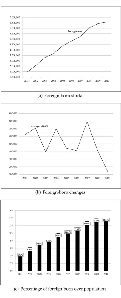
[INSERT TABLE1HERE] [INSERT FIGURE1HERE]
Figure 1 shows the evolution over time of the average stocks (top panel) and inflows (middle panel) of foreign-born and the share of foreign-born over population (bottom panel), between years 2001 and 2010 (long-differences). The share of foreign-born over total popu-lation rose almost 10 percentage points (from 4.8% to 14%) and the number of foreign-born
increased 237% (from 1,950,452 on the 1stJanuary 2001 to 6,579,121 on the 1stJanuary 2010). In every year of the period, the inflows of foreign-born were over 100,000 persons, and the average for the period is over 650,000. The three spikes in the inflows in figure2(b) corres-pond to three events described in Bertoli & Fern´andez-Huertas(2011): the 2000 law which allowed access to municipality public services when registered, the 2004 illegal immigration amnesty and the accession of Romania and Bulgaria to the EU in 2007.
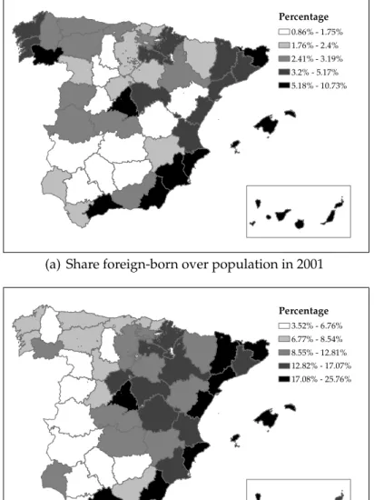
Figures A.1and A.2 in the Appendix display several maps which show the spatial dis-tribution of the stocks of foreign-born, the changes in the stock between 2001 and 2010, the share of foreign-born at the beginning and the end of the period and the total growth of foreign-born population. The different colours represent the 5 quantiles of the values of the mapped variable. The provinces on the coast and Madrid are the ones which have higher levels of immigrants and have received most of the inflows. In 2001 the highest shares of immigrants were also concentrated on the coastal provinces and Madrid, but in 2010 many inner provinces have high shares of immigrants. This is confirmed in the bottom panel of FigureA.2, in which we can observe that the provinces with fewer immigrants in 2001 (top panel inA.1) have been among the ones which have experienced the highest growth rate in the amount of foreign-born population between 2001 and 2010.
[INSERT TABLE2HERE] [INSERT FIGURE2HERE]
The top two panels of Figure 2show the evolution of the average price in Spain for the period of analysis. During the “housing boom” years (2001-2008) housing sale prices rose around 110% (around 16% per year), followed by the construction sector crisis in which average prices decreased around 12% in two years. Rental prices also increased importantly during this period, around one point above the general consumer price index (CPI) during 2001-2010. During the whole period rents raised around 35%20.
Construction of new dwellings also increased greatly during these years; between 2001 and 2010 5,312,245 new dwellings were built. The bottom panel of Figure2shows the evol-ution over time of the total and private housing stocks and Table2displays the total stock of dwellings in Spain during 2001-2010.
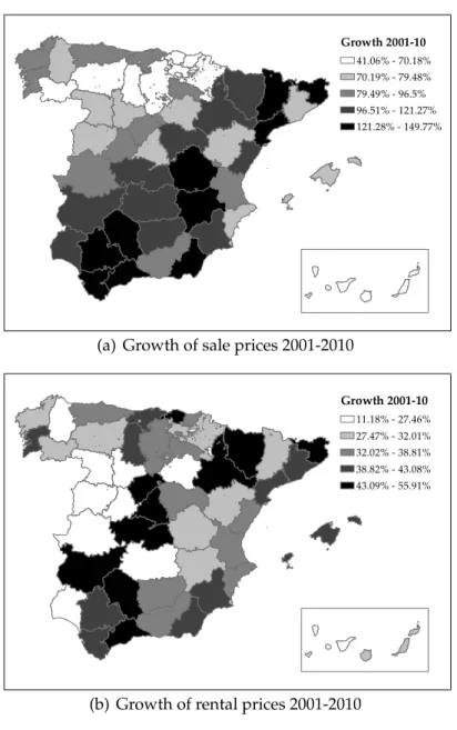
Figure A.3 in the Appendix shows the spatial distribution of the growth of prices and housing stock between 2001 and 2010. Sale prices increased substantially in all provinces. Some inner provinces (close to economic centers like Madrid, Barcelona, Sevilla or Valencia) experienced the highest growth rates in sale prices, probably due to the fact that prices were lower in those provinces in 2001. These seem to be also the locations in which construction has been concentrated, as shown in the bottom panel of the figure.
Most of the growth in prices and construction stopped in 2008 with the global economic crisis and between 2008 and 2010 prices have decreased and construction of new dwellings has virtually stopped, but their levels are still above the average values of the end of the 90s.
20Rental prices are based on the whole stock of properties available for renting (the already rented and the
just rented), and are tightly connected to national CPIs, so the scope for growth is smaller than in the case of sale prices. Conversely, the changes on house prices depend solely on new properties sold. Therefore, one can expect the increase on sale prices to be much more volatile than that of rents.
3
Results
3.1
Effect of immigration on house prices
Table3presents the ordinary-least-squares (OLS) results of the estimation of equation (1), for rental prices (top panel) and for sale prices (bottom panel)21. These results are obtained using data on annual changes on prices during the period 2002-2010 and data on the immigration ratio lagged one period (2001-2009). The number of observations is 450 (50 provinces times 9 years). In all specifications the standard errors are clustered at the province level, to allow for arbitrary correlation of the idiosyncratic shocks for a given province across time, and are robust to heteroskedasticity. All specifications include time dummies to control for national shocks. Different columns show results for different specifications which diverge in the area dummies, the area trends and in the controls that are included (geography, amenities, hous-ing supply and time-varyhous-ing controls). Specifications range from more to less demandhous-ing in terms of data variation: OLS results (column 1) to first differences province fixed effects model (column 7).
[INSERT TABLE3HERE]
The first column of Table 3 shows the results obtained by OLS. This is the simple raw correlation of the two variables (conditional on year dummies). The coefficients are 0.346 for rental prices and 0.588 for sale prices. In columns 2 to 5 I include region (NUTS2) dum-mies (2) and, subsequently, province geography and amenity controls (3), province housing supply controls (4) and province time-varying controls, lagged two periods (5). The coeffi-cient remains very similar for rental prices, but it increases for sale prices. In columns 6 I add region trends. The coefficients for both measures decrease. Column 7 presents the first differences province fixed effect estimates and includes time-varying province controls. This specification controls for province-specific time-invariant unobservables correlated with im-migration inflows and house price growth at the same time. The coefficients are larger than in column 6, but not statistically different from the specification with region dummies and trends (column 5).
The estimated elasticities of the changes in the immigration ratio on log changes of rental prices presented in the top panel of Table3range from 0.35 to 0.28. These magnitudes imply that an increase of the share of foreign-born on the original population of a province of 10% would cause an increase on the rental prices between 3.5% and 2.8% the following year. These numbers are much smaller than previous estimates found bySaiz(2007), which are around 8-10%. A possible explanation is the legal environment in Spain, as compared to the US case. In Spain the standard legal tenancy agreement for privately let properties establishes that the annual increase on the rental price would of the same amount as the change in the national CPI (during a standard contract length of 3 to 5-year)22. Given the existing legal limits to its growth, we can expect the impact of immigration on rental prices to be much more limited in this context23.
21For presentation purposes, I do not report the coefficients for the control variables and the fixed effects.
These results are of course available upon request
22Ley de Arrendamientos Urbanos 29/1994, del 24 de Noviembre de 1994.
23Most of the variation in rental price growth over time stems from newly signed tenancy agreements. The
smaller margin for adjustment of rents is illustrated in Figure2. Rents grow less than prices in the boom years but they also slow down less after 2009.
The bottom panel of Table3displays the results for the effect of immigration on housing sale prices. As expected, The estimates are bigger than in the case of rental prices, and range between 0.6 to 1.18. A 10% increase in the ratio would imply an increase in the sale price of around 12% on the following year. As for the case of the effects on rental prices, these estimates are also belowSaiz(2007) estimates.
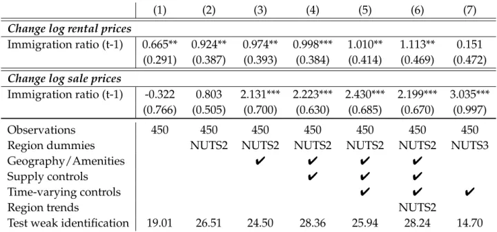
In order to be able to infer causal effects from the estimates of coefficient βin equation (1), I implement the IV strategy explained in section 2.3 and use the immigration ratio as defined in equation (3) to capture the impact of immigration on prices. As explained in sec-tion2.2, in this caseβcorresponds the long-run estimate and captures the combined impact of changes in demand, native location and in housing supply conditions24. Table4presents the results using the instrument as defined in equation (10). The predicted stocks and in-flows of foreign-born by nationality used in the computation ofimp pred FBstocki,t−1come
from the gravity model estimation, in particular from columns 1 and 4 in Table A.2. Year 1991 is used as the base year for the predicted location patterns of both natives and foreign-born. Table4has the same structure as Table3. As previously indicated, time fixed effects are included in all the specifications and the standard errors are clustered at the province level. The tables also display a test of the validity of the instruments (F-stat Kleibergen-Paap).
[INSERT TABLE4HERE]
The top panel of Table4presents the instrumental variable results for changes in rental prices and the bottom one, for changes in sale prices. As before, different columns show specifications with different sets of fixed effects and controls. The preferred specifications are those of columns 6 (which includes region fixed effects and trends) and column 7 (which includes province fixed effects). As expected, the standard errors increase when using in-strumental variables. For both house prices, the estimated effect of immigration inflows is larger than in Table3, in all specifications. This suggests that immigrants are moving, condi-tional on the controls and the area fixed effects, to provinces which are experiencing negative shocks in the growth of rental prices, and therefore the estimates of Table3 are downward biased. In all cases the instrument is strong. The Kleibergen-Paap F-stat is always over 10 and above the Stock-Yogo critical values.
For rental prices, the estimates elasticity in column 6 is around 1.1% and the coefficient is insignificant in column 7. The standard errors of both estimates are very similar but the coefficient decreases substantially when province fixed effects are included. As noted above, this specification is very demanding and, given that rental price growth correlates highly with inflation, it is likely that the province trends absorb most of the variation. For sale prices the elasticities range between 2.2 (column 6) and 3% (column 7). Both coefficients are not statistically different from each other (I reject the null hypothesis that the coefficients are different with a p-value of 0.48). As rental prices are insignificant in column 7, without loss of generality for sale prices, in the following sections I consider the results of column 6 (region dummies and trends) as the baseline.
Previous research has found estimates of positive sign and similar magnitude. The coef-ficients for both house prices are very similar to the IV elasticities estimated bySaiz(2007) and also comparable to the estimates byGonz´alez & Ortega(2013). As discussed above, the estimates obtained in this section do not take into account the relationship between
rant and native location decisions or adjustment of housing supply. They correspond to the causal reduced-form long-run impact. In the next section, I propose and apply a strategy to obtain the short-run (demand) impact on prices. The role of housing supply is explored in section3.4.
3.2
Effect of immigration on natives location
Section2.2discusses the issues related to the interpretation of the coefficient βwhen we do not take into account natives mobility. If immigrants do not affect native location choices, conditional on changes in supply25, βcaptures the effect of increased immigrant demand. However, if immigrants have a substantial effect on native location decisions, the long-run βwould be also affected by local changes in native demand. Depending on the sign of the effect, the short-run estimate would be above or below the long-run one. In order to uncover if this is the case, the first step is to study the relationship between natives and immigrant location decisions. In this Section, I estimate the causal relationship between native location and immigration inflows26.
[INSERT TABLE5HERE]
Table 5 shows the results of the estimation of equation (2). Columns 1 to 3 show the results using regional dummies and province fixed effects and columns 4 to 6 repeat the estimations using instrumental variables (instrument10). As the inflows of natives and im-migrants are contemporaneous, the time-varying controls are lagged one period with re-spect to time t. I find positive significant impacts of immigrant inflow on native inflow in all specifications. As before, when instrumenting the immigration ratio, the coefficients in-crease substantially. My preferred estimates are those of columns 5 and 6. These estimates predict that a for each 100 immigrants locating in a given province in a given year, between 45 and 60 natives located in the same province.
These findings suggest that natives and immigrants are contemporaneously locating in the same provinces. As discussed in section2.2, immigrants and natives might be heterogen-eous in skills levels and tastes. Immigrants might be regarded as complementary to natives and thus positively affect their location decisions. Besides enhancing productivity through improved task specialisation, immigrants might have desirable attibutes for natives. For ex-ample, if natives like ethnic diversity or if immigrants are specializing in producing goods and services which are desirable for natives.
Finding substantial immigrant-native co-location is different from most estimates in the literature27. The IV results Table 5 control for endogenous co-location of natives and im-migrants and thus the effect of imim-migrants on native location can be interpreted as causal.
Fern´andez-Huertas et al. (2009) find a comparable result for a long-differences estimation
25In the results of Section3.3, supply is already taken into account by including of time-invariant
supply-related controls. As shown in Section3.4, when I directly include house construction, the coefficients remain unchanged. For this reason, in the following I refer to the estimate that takes into account native mobility as the short-run effect without loss of generality.
26Other examples where the relationship between natives and immigration is explored are Card(2007),
Stillman & Mar´e(2008) andOrtega & Verdugo(2011) and issues about its estimation are discussed inPeri & Sparber(2011)
27Most of the literature compares immigrants and natives which have comparable occupation or skill levels
from population growth regressed on the immigration ratio for the period 2001-2008. Their prediction is of 11 natives for each 100 immigrants. They argue that this number is suffi-ciently small to have an impact on compensation or reinforcement of the impact of immig-ration inflows on the housing or the labour markets28. I find the size of the co-location to be substantially larger, suggesting that any impact of immigrants had on the housing markets would be amplified by the arrival of natives in the long run. I investigate this possibility in the following subsection.
3.3
Effect of immigration on house prices revisited
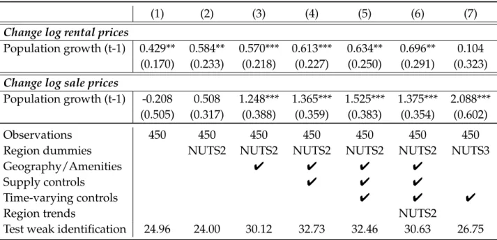
The estimates of the previous section suggest that the estimated coefficient βin equation (1) is captures the effects of increased demand from immigrants plus the increased demand from relocated natives. Here, I apply a methodology to isolate the effect that can be at-tributed to increases in immigration demand only. I use population changes as the main regressor in equation (1) and instrument it with expression (10). The instrument predicts exogenous foreign-born location, conditional on controls and fixed effects. By doing this, the population growth variable only captures the changes in population due to immigrant inflows and thus isolates the impact on house prices that stem from changes in foreign-born demand.
[INSERT TABLE6HERE]
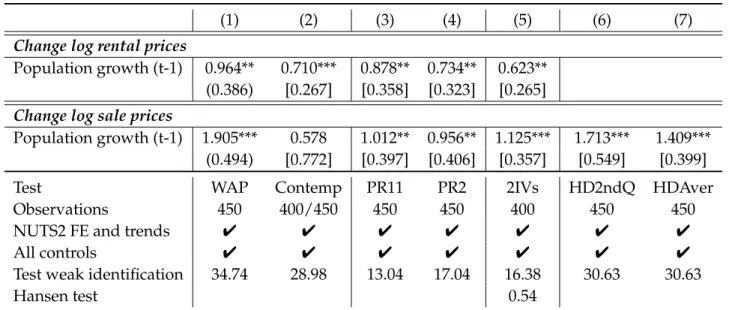
The results of using this strategy are shown in Table6. In this case, parameterβcaptures the causal effect of the growth in total population which is due to immigration inflow, be-cause to estimate the coefficient I only use the variation in population growth which stems from exogenous changes in the immigration ratio. In this setting, we expect the parameter β to be smaller than the one found in column 1, because it would be only capturing the effect of immigration through their effect on population changes. Conditional on controls and fixed effects, and on housing supply in some cases, this procedure separates the effect of foreign-born demand from the total long-run effect of immigration on prices.
The structure of the table is the same as in previous sections. The coefficients show the estimates of regressing population growth in t−1 (defined as changes in total population duringtdivided by population stock at the beginning oft) on log change of house prices. I instrument population growth usingIVmain imm ratioi,t−1as defined in (10). My preferred
specifications are those of columns 6 and 7 which use the most demanding set of area fixed effects and trends. The estimated elasticities in these columns are around 0.7% for rental prices and between 1.4 and 2.1% for sale prices. The coefficients estimated in Table 4 are between 45 and 60% larger, in line with the co-location effect estimated in the native mobility results in Table5. This suggests that, beyond the short-run impact, in the long-run, increased demand from natives has an additional impact on house prices. If we overlook the native-immigrant co-location, we largely overestimate the short-run impact of immigration.
The validity of these results relies on the assumption that, conditional on controls, the immigration instrument only affects prices via its effect on population changes. The
instru-28The difference in the results could be due to the fact that these authors do not use instrumental variables
in their estimation and they use long differences between 2001 and 2008, so they only use 52 observations. In fact, when they perform the estimation at the municipality level, using over 8,000 observations, they find very similar estimates to mine.
ment only aims to predict the location of immigrants, not natives. If the instrument directly affects native location, this assumption would be invalidated. In order for the strategy to be valid, I need to rely on the use of controls and on the fact that in the construction of IV (10) I use a prediction of native location in the denominator. Since the difference between the estimates of Tables4and6is very similar to the co-location effect found in the previous section, it is quite likely that the threats to the identification assumption are not of major relevance.
3.4
The role of housing supply
Depending on the level of housing supply elasticity, increases in housing demand following the immigrant inflows would have different effects on house prices. In this Section, I explore the role played by housing supply on potentially mitigating the increase in prices29. In the previous results, the role of housing supply it is already partially taken into account when I include time-invariant controls in the models to control for differential price growth trends based on some attributes of the provinces related to supply (proportion of rented properties in 2001, proportion of empty houses in 2001, share of developable land in 2000 and regu-latory index in 1999). In this section, I directly investigate the mitigating impact that supply changes might have on house prices by including the growth in the stock of (private) dwell-ings as an additional control variable.
[INSERT TABLE7HERE]
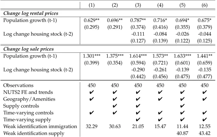
The results are presented in Table 7. I focus on the specification that includes region fixed effects and trends, but the results using province fixed effects are very similar. As my aim is to estimate the impact of immigration demand changes, I present the results using population growth (due to immigration inflows) and not the immigration ratio, in-strumented as explained in section3.3. Column 1 shows the results using region dummies and trends and all the controls except the supply time-invariant controls. In column 2 I introduce these variables to replicate the results from column 6 in Table 6. The coefficient of population growth barely changes when adding these controls. In Column 3 I include the time-varying supply control (log change housing stock in t−2). Now the coefficient of population growth captures the impact of changes in immigrant demand conditional on housing supply changes. The coefficient of population growth increases, suggesting that, if we not take supply changes into account, it is downward biased. The coefficient for housing construction is negative, suggesting that larger increases in supply yield lower increases in house price growth, conditional on changes in immigrant demand. However, it is insignific-ant. In column 4 I explore if the insignificance of the time-varying housing supply coefficient is due to lack of variation when controlling for time-invariant supply characteristics so I ex-clude these from the specification. The results are very similar to those of column 3 and suggest that housing supply growth has not direct effect on house price changes conditional on population growth.
Using the growth of housing stock as an additional control variable in Table 7is highly problematic. Even if lagged two periods with respect to the outcome variable, and one period with respect to the population growth, this variable is likely to be endogenous.
Un-29This analysis applies mostly to the effect on sale prices. The impact of housing construction on rental prices