O R I G I N A L P A P E R
Fast parallel genetic programming: multi-core CPU
versus many-core GPU
Darren M. Chitty
ÓSpringer-Verlag 2012
Abstract Genetic Programming (GP) is a computation-ally intensive technique which is also highly parallel in nature. In recent years, significant performance improve-ments have been achieved over a standard GP CPU-based approach by harnessing the parallel computational power of many-core graphics cards which have hundreds of pro-cessing cores. This enables both fitness cases and candidate solutions to be evaluated in parallel. However, this paper will demonstrate that by fully exploiting a multi-core CPU, similar performance gains can also be achieved. This paper will present a new GP model which demonstrates greater efficiency whilst also exploiting the cache memory. Fur-thermore, the model presented in this paper will utilise Streaming SIMD Extensions to gain further performance improvements. A parallel version of the GP model is also presented which optimises multiple thread execution and cache memory. The results presented will demonstrate that a multi-core CPU implementation of GP can yield perfor-mance levels that match and exceed those of the latest graphics card implementations of GP. Indeed, a perfor-mance gain of up to 420-fold over standard GP is dem-onstrated and a threefold gain over a graphics card implementation.
Keywords Genetic Programming Multi-core CPU Many-core GPU
1 Introduction
Genetic Programming (GP) (Koza 1992) is a well-estab-lished, highly effective machine learning approach. How-ever, a key drawback of the technique is its computational intensity which has been been a limiting factor on the effectiveness of GP for machine learning when considering large problems or datasets. The primary reason behind this computational complexity is that GP is a population-based technique requiring the evaluation of tens of thousands of candidate solutions. Moreover, these candidate solutions need to be evaluated by interpreting them repetitively over a large number of fitness cases.
To address this issue there have many attempts to improve the speed of GP from machine code, sampling and caching subtrees to the exploitation of parallel hardware. However, recently graphics processing units (GPUs) have emerged as a considerable parallel computing resource through hundreds of processing cores providing large-scale parallelism on desktop computing platforms. Subsequently, the primary method of achieving fast GP has concentrated on utilising graphics cards on which considerable speedups in the execution time have been achieved. However, the multi-core CPU is a neglected resource and is capable of achieving similar results. Indeed, Lee et al. (2010) dem-onstrated that many of the speedups cited in the literature for graphics card technology over CPU approaches for a series of computationally intensive algorithms were in fact overstated. The CPU comparison algorithm often did not exploit the full capability of a modern CPU. But, by fully utilising a CPU, in some cases, better performance could be achieved by a CPU approach than that of a graphics card. Little work has been done on improving the execution speed of CPU-based GP by fully harnessing the CPU hardware. However, through the exploitation of the cache D. M. Chitty (&)
Department of Computer Science, University of Bristol, Merchant Venturers Bldg, Woodland Road,
Bristol BS8 1UB, UK
e-mail: [email protected] DOI 10.1007/s00500-012-0862-0
memory, 128 bit registers and the multi-core capabilities of these processors, the performance of GP can be signifi-cantly improved on a CPU. The work presented in this paper will seek to address this issue. Section2will provide an overview of parallel GP focusing on the achievements to date of graphics card-based GP. Section 3 will describe cache memory and how to best exploit it for the purposes of GP introducing a new GP model. Section4will discuss the 128 bit registers on modern CPUs and demonstrate their application to GP. Section 5 will present a well-uti-lised methodology to optimise the cache memory and the re-interpretation of candidate solutions known asblocking and apply this to the new GP model. Section6 will dem-onstrate the use of the multiple cores of a modern CPU for population-parallel GP whilst maintaining optimal perfor-mance from the cache memory. Section 7 will introduce some further enhancements and Sect. 8 will provide a direct comparison between the CPU GP model presented in this paper and the latest graphics card approaches.
2 Background
Genetic Programming can be considered an embarrass-ingly parallel technique. Indeed, the technique is ideally suited to parallel technology in two respects. Firstly, a population of candidate solutions can be evaluated over the set of fitness cases completely independently of each other in parallel, a ‘‘population parallel’’ approach. Secondly, fitness cases can also be considered independently from each other in parallel, a ‘‘data parallel’’ approach. Tufts (1995) used this approach for a parallel implementation of GP. The first implementations of parallel GP utilised the parallel hardware of supercomputers. Juille and Pollack (1996) implemented a Single Instruction Multiple Data (SIMD) model of GP whereby multiple candidate solutions were evaluated in parallel, using a MASPar MP-2 com-puter. Andre and Koza (1996) used a network of trans-puters with a separate population of candidate solutions evolved on each transputer with migration between the populations, an island model. Niwa and Iba (1996) implemented a distributed parallel implementation of GP, also using an island model, executed over a Multiple Instruction Multiple Data (MIMD) parallel system AP-1000 with 32 processors. In fact, the island model, also known as a multi-population model, has been frequently used in parallel GP implementations as the communication between processors in a supercomputer is a considerable bottleneck. Using a separate population per processor means processors can operate for longer in isolation before needing to communicate to other processors thus reducing the communication bottleneck. Ferna´ndez et al. (2003) conducted a review of multi-population techniques
demonstrating both improvements in solution quality and computational effort over single populations. Punch (1998) also reviewed multi-population parallel GP demonstrating that different problems have differing performances from the use of a multi-population GP model. Folino et al. (2003) extended the multi-population model another step by introducing a cellular or grid model whereby popula-tions occupy a grid and can only reproduce with neigh-bouring populations. This means genetic changes will only slowly permutate through the system. Gustafson and Burke (2006) developed a multi-population parallel GP model whereby differing species were identified during the evo-lution process and these were spun off to form their own sub-population.
More specialised hardware in the form of Field Pro-grammable Gate Arrays (FPGAs) have also been harnessed by the GP community to parallelise the process. For instance, Martin (2001) used a special C compiler to run GP on FPGAs whilst Eklund (2003) used an FPGA simu-lator to demonstrate that GP could be run on FPGAs to model sun spot data. The Internet has also been used to facilitate parallel GP by distributing a population of indi-viduals for evaluation across many computers. Chong and Langdon (1999) utilised Java Servlets to distribute genetic programs across the Internet whilst Klein and Spector (2007) used Javascript to harness computers connected to the Internet for the purposes of GP without explicit user knowledge.
Implementations of parallel GP have been relatively few though due to the necessity of access to specialised parallel hardware. However, in recent years parallel hardware has become commonplace in standard desktop computers. In order to continue to achieve improved performance from CPUs, micro-processor manufacturers have used multi-core technology whereby each CPU has a small number of processing cores enabling multiple instructions to be exe-cuted in parallel. Modern CPUs, such as Intel’s i7 pro-cessor, have four processing cores each with the same processing capability of a standard single-core processor. However, multi-core technology has been adopted to a much greater extent by graphics card manufacturers. Consumer demand for realistic graphics within computer games has caused the computational power of Graphical Processing Units (GPU) to increase much more rapidly than the CPU. This has been achieved though the use of a massively parallel architecture whereby there are hundreds of processing cores operating at a low frequency. A GPU is capable of limited MIMD operation using a small number of multi-processors. However, the processing cores are separated into groups under each multi-processor and each group operate in a SIMD manner when executing a kernel. This architecture is well suited to the processing of graphics. However, the computational power of these
GPUs was quickly recognised by the scientific community and a field of research was established known as General Purpose Computation on Graphics Processing Units (GPGPU). This has led to significant gains in the execution speed of many computationally intensive algorithms through the use of these many-core GPUs.
Subsequently, the computational power of GPUs has led to parallel GP being rapidly implemented to take advantage of this technology. Chitty (2007) and Harding and Banzhaf (2007) were the first to develop implemen-tations of GP that operated on graphics card technology. Both authors identified that the greatest computational aspect of GP is the evaluation phase and thus both approaches used the parallelism of the GPU to sequen-tially evaluate candidate solutions on multiple fitness cases simultaneously, a data parallel approach. This provided significant gains in computational speed over a standard GP implementation of up to 95-fold for problems with large numbers of fitness cases. However, for problem instances with few fitness cases a worse performance was observed. Both these approaches used a compiled approach whereby a candidate solution was translated to a GPU program which then operated over all the fitness cases using the inherent parallelism of the stream pro-cessors. Langdon and Banzhaf (2008) later used the RapidMinds toolkit to develop a more traditional inter-preted approach using a stack system. However the computational cost of the interpreter led to only a 12-fold improvement.
In 2006 NVidia developed a GPU toolkit known as the Compute Unified Device Architecture (CUDA) to facilitate the use of GPU technology for general computational tasks. CUDA has since been extensively used to create inter-preted approaches to GP using GPUs. Robilliard et al. (2008) used the toolkit to create an interpreted system known as BlockGP. This approach used a population parallel and data parallel approach whereby candidate solutions were parallelised across the multi-processors of the GPU whilst the fitness cases were parallelised on the stream processors operating under each multi-processor. An 80-fold improvement over a CPU-based approach was demonstrated for a symbolic regression problem. Langdon and Harrison (2008) also used the CUDA system to develop an interpreted GP approach using graphics hard-ware for a bioinformatics problem demonstrating a sig-nificant speedup over a CPU approach. Moreover, Langdon developed a measure for assessing the speed of a GP implementation known as Genetic Programming Opera-tions per Second (GPops). The Langdon approach achieved a speed of 250 million GPops versus a CPU alternative that only ran at 13 million GPops.
The latest interpreter-based approaches to GP on graphics hardware have evolved to exploit to a greater
extent the inherent parallelism available. Robilliard et al. (2009) made improvements to BlockGP with program optimisations and utilisation of GPU fast memory which improved the approach threefold. Using this approach, a maximal speed of 4.7 billion GPops for a sextic regres-sion problem was obtained, an approximate 1609
speedup over a CPU-interpreted approach to GP. Lang-don (2010) used a similar approach with the 37 multi-plexor problem achieving a maximal speed of 254 billion GPops. However, this uses bit-level parallelism as the problem under consideration is a boolean problem. Thus using 32 bit floats an extra 329parallelism is achieved. Thus, for comparison purposes with other classical problems, this actually translates to 8 billion GPops. Harding and Banzhaf (2009) devised a distributed tech-nique whereby 14 computers equipped with graphics cards were utilised to run GP. Each system handled part of the dataset and used a compiled approach whereby a candidate solution was translated into a CUDA kernel. A speed of 2.25 billion GPops was achieved for the full KDDcup dataset and 12.7 billion GPops for the evolution of image filters. Cano et al. (2012) evaluated three dif-fering GP approaches using both a multi-core CPU and two GPUs. The maximal gain achieved was an 8209
speedup over a serial Java CPU approach when consid-ering the Poker dataset. Lewis and Magoulas (2009) interleaved CPU operations with the evaluations on a GPU to achieve a maximum performance gain of 3.8 billion GPops. Maitre et al. (2010) achieved significant speedups even when using small numbers of fitness cases by using efficient hardware scheduling in CUDA. A speedup of up to 2509 is achieved over a serial CPU implementation.
However, the computational power of the CPU has been largely ignored by the GP community. Perhaps this is because modern CPUs can achieve approximately 100 GFlops compared to the latest GPUs which can achieve over 1,000 GFlops, a tenfold improvement. Fully exploit-ing this power is difficult though due to the small amount of fast memory available to each thread of execution. Moreover, branching statements, such as conditional statements in a GP tree, can affect the execution speed due to the SIMD nature of the stream processors operating under each MIMD multi-processor. Finally, a small per-formance limit is the requirement to copy data to and from the GPU. A point also worth noting is that GPU approaches in the literature make comparisons with basic versions of CPU-based GP biasing the speedups demonstrated. The work presented here will address this imbalance. Moreover, the CPU will be shown to be a viable alternative to the massively parallel graphics card technology both matching and exceeding the performance of the GPU implementa-tions of GP.
3 Cache efficient genetic programming 3.1 Cache memory
Originally there was little to choose in terms of computa-tional time between accessing memory or executing instructions on the CPU. Both microchips operated at the same clock frequency. However, in recent years, the clock frequency of processors has increased dramatically whilst the clock frequency of memory has not. This has had the effect of making memory accesses appear much slower in comparison to instruction execution. It is possible to create memory chips with the same clock frequency as CPUs but the resulting product would be highly expensive and hence unviable for modern memory requirements. However, creating small amounts of memory that operate at a similar clock frequency as the CPU is a viable option.
This fast memory is relatively small and hence does not operate in the same manner as conventional memory. Indeed, it is not directly accessible but is instead admin-istered by the processor directly. In essence, this fast memory consists of direct copies of memory locations within the main memory. When a memory location is requested, if it has been copied to the faster memory the access speed will be considerably faster. Since this faster memory consists only of copies of memory locations within the main memory, it is known as cache memory.
Whenever a memory location is requested from the main memory a copy is placed into the cache memory. More-over, it was recognised that in many cases, when a memory location is accessed, the neighbouring memory locations will also shortly be accessed. This is certainly true for a sequential algorithm iterating over an array. Thus to maximise efficient use of cache memory, whenever a memory location is accessed, the contents are copied to the cache along with neighbouring memory locations. The amount of neighbouring memory locations copied to the cache memory equates to thecache linesize. This is typ-ically 64 bytes in size which is the equivalent of 16 single precision floating point values or 8 double precision floating point values. As the cache memory is of limited size, whenever memory locations are copied into the cache, room must be made. Hence, the memory locations whereby the period of time in which they were last accessed is the greatest, are removed to make room for the new values. This is known as a Least Recently Used (LRU) replace-ment strategy.
Modern processors are now generally equipped with hierarchical cache memory whereby there are several lay-ers of cache memory with differing access speeds and size. Indeed, the i7 processor from Intel comes with three hierarchical levels of cache, L1, L2 and L3. L1 is the fastest cache memory but also the smallest with only
64 Kb. L2 is larger in size with 256 Kb but slightly slower than the L1 cache. The L3 cache is the largest at 8 Mb but also the slowest although still considerably faster than accessing main memory. Furthermore, the i7 CPU is a multi-core processor with four cores. Each of these cores has its own L1 and L2 caches but the L3 cache is shared between the four cores. The hierarchical cache model operates by making copies of main memory locations into the L1 cache. If room is required, then copies of memory locations whereby the period of time since they were last accessed is the greatest are moved into the L2 cache. Again, if room is needed in the L2 cache then the same process occurs to move copies of memory locations into the L3 cache. Similarly, if space is required in the L3 cache then copies of memory locations accessed the greatest time ago are removed from the L3 cache memory. Whenever a memory location is requested each cache level is checked in succession for the requested memory location before accessing the slower main memory.
A final aspect of consideration is that the L2 and L3 caches are data only cache memory. However, the L1 cache is divided into both data and instruction-level cache memory. The instruction-level cache contains recently executed instructions in order to reduce the computational time for the fetch execute cycle. Thus repeatedly executing the same instructions will be faster than executing a wide range of instructions. For a detailed look at cache memory, Smith (1982) provides a comprehensive guide to cache memory.
3.2 Modifying GP to exploit cache memory
Traditional GP (Koza 1992) operates by evaluating each candidate solution of a population over a set of fitness cases. In order to achieve this, GP interprets the genetic code of each candidate solution executing the specific instructions required at each stage of the candidate solu-tion. With traditional tree-based GP, candidate solutions are represented as a tree structure whereby results from lower branches form inputs to the higher level branches. Computer systems are not designed to execute programs in a tree form. Thus, in order to evaluate a GP tree, an interpreter must be used to correctly execute the right GP operator at each node of the tree. Moreover, this inter-preter, to be able to correctly evaluate any GP tree, oper-ates in a recursive manner. Furthermore, a stack must be used to store the results of GP operators such that they can be retrieved by GP operators at a higher level in the tree as input arguments.
Using a stack to interpret a GP tree operates in the following manner. Whenever a GP operation is executed, the input arguments to the operator are ‘‘popped’’ off the stack. The result from the GP operator is ‘‘pushed’’ on to
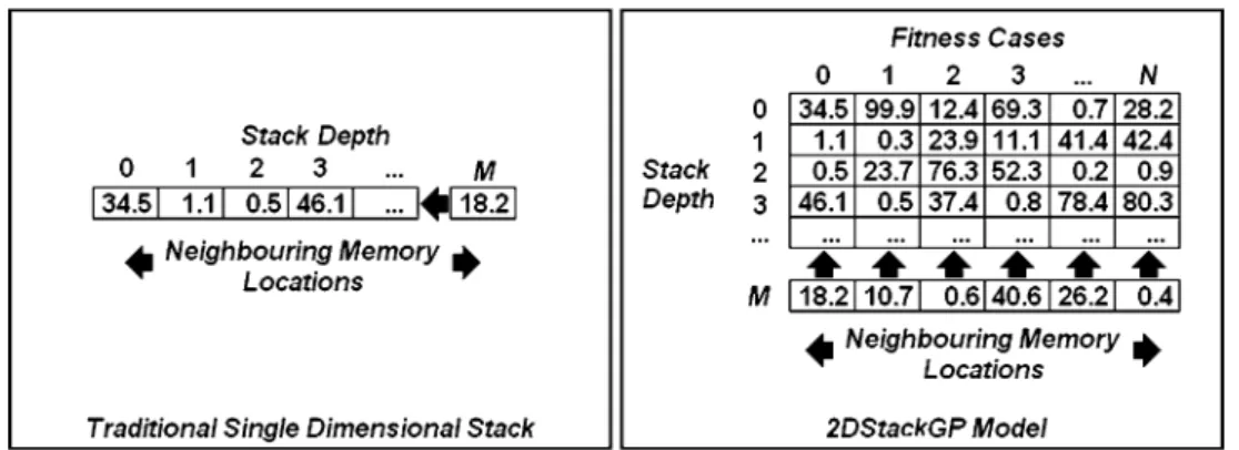
the stack. Terminal values are also ‘‘pushed’’ on to the stack. The stack operates in a Last In First Out (LIFO) model such that the last value ‘‘pushed’’ on to the stack is the first to be ‘‘popped’’ off. This stack is generally represented as a single dimensional array with a pointer to the position of the top of the stack. Figure1provides an illustration of a stack used by traditional GP. A candidate solution needs to be reinterpreted for every fitness case in the set.
However, this method of reinterpreting a candidate solution for each and every fitness case in a sequential manner is both inefficient and does not fully exploit the potential of a CPU’s cache memory. Since each fitness case is considered in isolation, inputs from a given dataset will always need to be retrieved from the slower main memory. Moreover, only limited stack values will be retrieved from the faster cache memory as stack values are retrieved in reverse order. Hence, in some cases, stack values could have been pushed out of the cache.
In order to better exploit the cache memory an alterna-tive model is required. Indeed, since whenever a memory location is accessed, the neighbouring locations are loaded into the cache memory perhaps an iterative approach can be considered. In this model, whenever a GP operator is executed it iterates over all the fitness cases instead of considering a single fitness case. To achieve this, a two-dimensional stack will be necessary in order to store all the results from every fitness case under consideration by a GP operator and also to provide the inputs to subsequent GP operators. Computer memory is one dimensional in nature thus multi-dimensional arrays are represented in memory as a single dimension. Hence, to maximise cache memory utilisation, the first dimension should consist of the maxi-mal depth permissable. The second dimension should consist of the number of fitness cases. Figure1 shows the traditional single dimensional stack and a new 2D stack representation. This demonstrates how the 2D stack is represented in memory and thus how for each level of the
stack, values for each fitness case are neighbours. This may seem a considerable memory overhead. However, using a 32-bit floating point type with a stack of maximum depth of 50 for 100,000 fitness cases will involve only using approximately 19 Mb of main memory, well within mod-ern main memory sizes.
The 2D stack GP model will operate by only interpreting each candidate solution a single time. When a GP operator is required to be executed it will now iterate over all the fitness cases storing the results across the stack. Conse-quently, each GP operator now consists of a for loop iterating over all the fitness cases. Algorithm 1 demon-strates how the GP addition operator will now function within the new GP model. Clearly, the cache memory will now be better exploited as when the first iteration of the for loop occurs, the neighbouring inputs from the stack for fitness case two, three, etc. will be loaded into the cache memory. Thus when the second iteration of thefor loop occurs, the required input values from the stack are already held within the cache memory and thus retrieving these values is considerably faster. In addition to better exploit-ing the cache memory, the same instruction is now exe-cuted repeatedly for every fitness case. Consequently, the instruction level cache in L1 is exploited to maximal effect. Finally, as each candidate solution is only interpreted a single time, a considerable efficiency saving is made. Interpreting programs is computationally costly as it involves many conditional statements and branching. The new GP model presented here will be referred to as 2DStackGP.
Fig. 1 The two differing stack models represented by a single dimensional array and two-dimensional array in memory. With the single dimensional stack, each level is a neighbouring memory location of the last. With the two-dimensional stack model, the stack
values for each fitness case need to be neighbouring memory locations for optimal cache performance. Hence the stack needs to be transposed for this to be the case
It should be stated that this model will only be useful in instances when the same instructions are executed for every fitness case. The types of problems this suits are data processing tasks rather than simulations such as robot planning tasks. Moreover, GP trees with dynamic loops dependant on the data from each fitness case are not suit-able. However, conditionals can be considered as the unnecessary branches can still be interpreted but the results masked. The technique has been used here with tree-based GP but it can be considered that the technique would work equally well with other GP variants whereby GP operators are executed repeatedly for many fitness cases. Moreover, this 2DStackGP model can even be considered at a more general level for any interpreter-based technique which involves processing a large dataset.
3.3 Initial results
In order to properly evaluate the performance of the 2DStackGP model, four standard problems are considered. Two classification problems, a sextic regression problem and a boolean problem.
Sextic polynomial regression problemThis problem is a symbolic regression problem with the aim of establishing a function which best approximates a set of data points. In this case the set of data points is generated by the poly-nomialx6-2x4?x2(Koza1992). The function set used is *, /,?,-,Sin,Cos,Log,Exp. The data point input values are random values within the interval of [-1,?1]. For this problem 100,000 fitness cases are used.
Shuttle classification problemThis problem is a classi-fication problem whereby the goal is to establish a rule that can correctly predict the class of a given set of input values. In this case the data is the NASA Shuttle StatLog (King et al.1995) available from the machine learning repository (Frank and Asuncion 2010). Both the test and training datasets are used providing a total of 58,000 fitness cases. There are 10 classes within the dataset with 75 % belonging to a single class. There are nine input variables for each class. The function set consists of *, /,?,-, [,\,==, AND, OR, IF and the terminal set consists of
X1;. . .;X9;-200.0 to 200.0.
KDDcup intrusion classification problemThis problem is also a classification problem. In this case the dataset is the test data from the KDD Cup 1999 problem (1999) with the aim to correctly classify potential network intrusions. The dataset used is the test data which consists of 494,021 fitness cases with 41 input values. The function set consists of ?, -, *, /, [, \, = =, AND, OR, IF, Sin,Cos, Log,Exp and the terminal set consists of X1. . .X41,
-20,000.0 to 20,000.0. There are 22 classes within the dataset.
Boolean 20-multiplexor problem This is a standard Boolean problem used in GP (Koza 1992). The goal is to establish a rule which takes address bits and data bits and outputs the value of the data bit which the address bits specify. The function set consists of AND, OR, NAND, NOR and the terminal set consists of A0-A3, D0-D15. Every potential option is considered such that there are 220 fitness cases which is 1,048,576. However, in real terms this can be reduced as bit-level parallelism can be utilised such that each bit of a 32-bit variable represents a differing fitness case. Thus, the number of fitness cases are effec-tively reduced to 32,768.
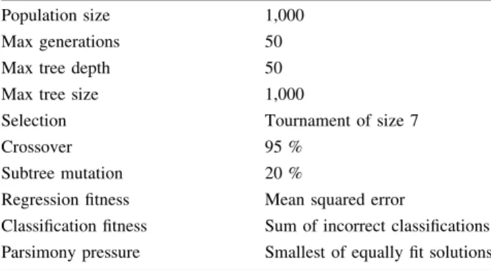
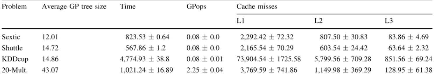
The results in this paper were generated using an i7 2600 Intel processor running at 3.4 GHz with four processor cores each able to run 2 threads of execution indepen-dently. Each of the four cores has an L1 and L2 cache of size 64 Kb and 256 Kb, respectively. There is also an 8 Mb L3 cache which is shared between the four processor cores. The i7 processor has a theoretical floating point perfor-mance of 109 GFlops. The algorithms used were written in C?? and compiled using Microsoft Visual C?? 2010. Table1 provides the GP parameters that were used throughout this work. Each test was averaged over 25 runs. Table2 demonstrates the performance of the standard approach to GP and Table3 the 2DStackGP model. The execution speed of the two approaches is shown in terms of execution time and also billion genetic programming operations per second (GPops). The GPops measure was introduced by Langdon and Harrison (2008) and is calcu-lated by multiplying the total number of nodes of every candidate solution evaluated by the number of fitness cases divided by the execution time in seconds. In addition, Tables2 and3also show the cache misses for each cache level measured in millions. These were obtained by accessing the Model Specific Registers (MSRs) on the i7 processor which can be setup to count events such as cache misses. However, this measure is system wide and as the operating system has many underlying processes the cache miss results are subject to some variance.
Table 1 GP parameters used throughout paper Population size 1,000
Max generations 50
Max tree depth 50
Max tree size 1,000
Selection Tournament of size 7
Crossover 95 %
Subtree mutation 20 %
Regression fitness Mean squared error
Classification fitness Sum of incorrect classifications Parsimony pressure Smallest of equally fit solutions
From Table2it can be seen that the standard technique achieves a speed of 80 million GPops for the standard problems. For the 20 multiplexor problem which uses bit-level parallelism, a rate of 2.25 billion GPops is achieved. From Table3 it is clear that the 2DStackGP model is a considerable improvement. The evaluation of candidate solutions by using a 2D stack to execute each GP operator over all the fitness cases in a single step achieves an approximate speed of 500 million GPops for the standard problems. For the multiplexor problem this rises to 18 billion GPops through bit-level parallelism. Thus an aver-age sevenfold improvement in computational speed over a standard approach to GP is achieved by improving effi-ciency and exploiting the cache memory. This can be observed by analysing the cache misses. The standard approach has considerably more cache misses across all cache levels especially L3 which means the main memory has to be accessed a significantly increased amount which is a time-consuming operation. As a percentage of execu-tion time there is increased variance in the results from the 2DStackGP model but the variance is still low.
3.4 Further reducing the memory overhead
As described in the previous section, a considerable time cost in the execution speed of the GP algorithm is reading and writing to memory. Thus any step that can reduce this overhead will provide a significant increase in computa-tional speed. Currently, terminal values based on the given dataset or constant terminal values are ‘‘pushed’’ onto the
stack for each of the given fitness cases. However, this is not necessary when considering dataset terminal values. Transposing the dataset such that the first dimension con-sists of the dimensions of the dataset and the second dimension the fitness cases will better exploit the cache memory as has been achieved with the stack. Moreover, this transposed dataset now matches the 2D stack repre-sentation in memory. Since the stack is a set of pointers to memory locations, instead of copying the data onto the stack for every fitness case, the stack memory pointer can simply be pointed to the required dimension of the dataset held within the memory. This is a considerable improvement in compu-tational cost when compared to copying each individual value from the dataset onto the stack. Once the terminal dataset input has been effectively ‘‘popped’’ off the stack the original pointer to the stack memory can be restored.
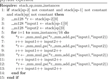
Further improvements can also be achieved when con-sidering constant terminal values as only a single value needs to copied onto the stack. If a level of the stack is labeled as containing a constant value then a GP operator need only use the first element of the given stack level. Clearly, the same constant value is used for all fitness cases. Algorithm2shows an example of the modifications required for the example addition operator. Since there are two inputs to an addition, there are four possible outcomes. Note that the second and third branches do not iterate through one of the stack inputs. If both the inputs are labeled as constant terminals then noforloop is required. A simple single addition is calculated and placed on the stack which is also flagged as a constant. Thus, a further Table 2 The execution timings with standard deviation for a standard GP approach
Problem Average GP tree size Time GPops Cache misses
L1 L2 L3
Sextic 12.01 823.53±0.64 0.08±0.0 2,292.42±72.32 807.50±30.83 83.86±4.69 Shuttle 14.72 567.86±1.2 0.08±0.0 2,165.54±70.29 603.54±24.42 63.64±2.32 KDDcup 14.86 4,774.93±38.8 0.08±0.01 73,904.54±1725.58 5,799.56±709.28 851.56±69.24 20-Mult. 43.07 1,021.24±16.89 2.25±0.04 3,769.59±741.86 1,149.98±369.29 128.95±61.38 Time is measured in seconds, GPops in billions and cache misses are measured in millions
Table 3 The execution timings with standard deviation for the 2DStackGP model
Problem Time GPops Cache misses Overall speedup
L1 L2 L3
Sextic 146.08±0.38 0.42±0.0 710.58±88.28 304.98±25.56 22.20±1.8 5.649 Shuttle 80.68±0.57 0.54±0.0 302.22±53.1 156.47±17.91 11.74±1.86 7.049 KDDcup 628.79±21.78 0.6±0.02 3,193.25±64.14 1,230.26±29.35 392.78±9.07 7.599 20-Mult. 124.66±2.87 18.48±0.41 535.52±27.56 242.12±8.63 17.40±1.32 8.199 Time is measured in seconds, GPops in billions and cache misses are measured in millions
reduction in the memory operations is achieved at the GP operator level as only a single value needs to be loaded from the memory when considering constants.
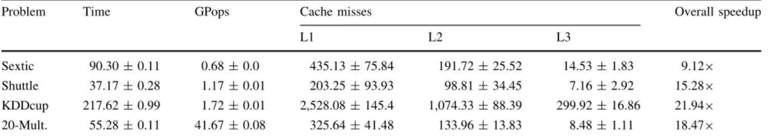
Table4 demonstrates the further improvements in com-putational speed that the dataset and constant value modifi-cations to the 2DStackGP model achieve. Comparing the results of Table4with those from Table3, it can be seen that the number of cache misses across all levels have reduced. This, along with a reduction in computation operations, has translated into a significant improvement on the speed of the evaluation of candidate solution. An average rate of 1.2 billion GPops is now achieved for the standard problem cases and 42 billion GPops for the boolean multiplexor problem. This is an average performance gain of 2.239over the original design of the 2DStackGP model and an average 16.29improvement over the standard GP approach to evaluating candidate solu-tions. The KDDcup problem benefited the most and this is most likely to be due to the large volume of data associated with this problem instance. In addition, the variance as a percentage of execution time for the improved 2DStackGP model is considerably reduced too.
4 Exploiting streaming SIMD extensions for GP Before the advent of multi-core processors Intel developed a limited form of parallelism in order to provide additional computational power. In 1999, Intel introduced processors with a small number of 128 bit registers available on their CPUs. These registers enabled four 32-bit values or two 64-bit values to be placed in these registers. When an instruction is executed on these 128-bit registers a limited level of parallelism can be achieved. This parallelism is known as Single Instruction Multiple Data (SIMD) paral-lelism. Indeed, Intel also made available an instruction set for exploiting these 128-bit registers known as Streaming SIMD Extensions (SSE) (Intel Architecture Software Developer’s Manual Volume 2: Instruction Set Reference 1997).
The SIMD nature of the SSE instruction set ideally suits the 2DStackGP model presented in Sect.3. Recall that each GP operator now iterates over all the fitness cases in a single step. Essentially, this constitutes a single instruction executed over multiple data cases which is a SIMD model. To exploit the SSE instruction set for GP requires each GP operator to load four fitness cases into a 128-bit register and execute an SSE instruction upon the contents of the register. For tradi-tional GP this is not possible using a single dimensional stack.
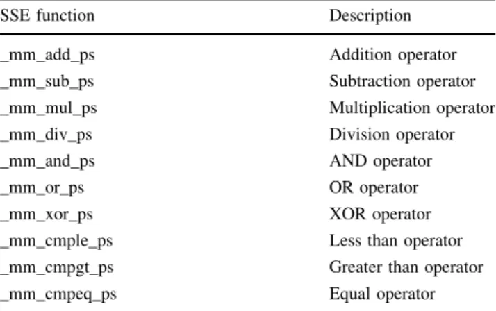
Table5 provides an overview of the SSE instructions that are utilised within this work. The ‘‘ps’’ extension at the end of each function name denotes that the operation in question is parallel scalar, thus it operates on four 32-bit floating point values. Functions that the GP implementation uses but are not available in the SSE instruction set are the trigonometric functionsSin,Cos, Log andExp. For this reason approximations were used throughout this paper such that an SSE version could be constructed. In order to use the SSE instruction set, the declared memory areas such as the stack and the given dataset must be 16-bit aligned. In C?? the _align_calloc function achieves this. Furthermore,
Table 4 The execution timings with standard deviation for the improved 2DStackGP model
Problem Time GPops Cache misses Overall speedup
L1 L2 L3
Sextic 90.30±0.11 0.68±0.0 435.13±75.84 191.72±25.52 14.53±1.83 9.129 Shuttle 37.17±0.28 1.17±0.01 203.25±93.93 98.81±34.45 7.16±2.92 15.289 KDDcup 217.62±0.99 1.72±0.01 2,528.08±145.4 1,074.33±88.39 299.92±16.86 21.949 20-Mult. 55.28±0.11 41.67±0.08 325.64±41.48 133.96±13.83 8.48±1.11 18.479 Time is measured in seconds, GPops in billions and cache misses are measured in millions
declared variables must be of size 128 bits for which the __mm128 variable can be used. Direct casting can be achieved between an array of floats and the __mm128 variable type.
Algorithm3 provides an SSE implementation of the addition GP operator. Note that the actual addition sign has been substituted for the _mm_add_ps SSE func-tion. Also, observe that a direct cast is made from the stack pointer to an__m128SSE variable pointer. Also note that the result is incremented by one at each iter-ation of the for loop, but the loop now only iterates for a quarter of the fitness cases. This is due to the __m128 variable type representing four floating point values. When this variable is incremented it points to the next four 32-bit floating point values held in memory.
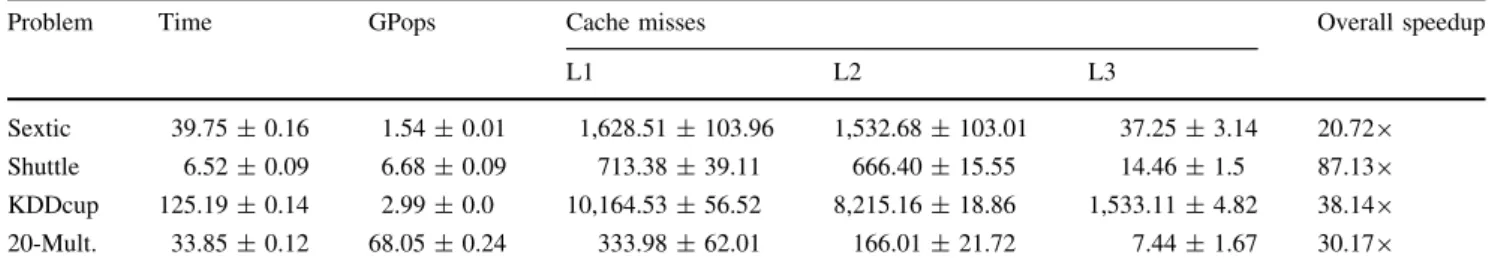
Table6 details the results achieved from utilising the SSE instruction set. The Shuttle classification problem achieved the best performance gain from using the SSE instruction set. The KDDcup and sextic regression problem achieved a slightly lower improvement. A key reason for this is that the SSE instruction set does not provide trigonometric functions. Consequently, approx-imations were used which did not translate efficiently to the SSE instruction set. On average a threefold improvement in execution speed has been achieved over the improved 2DStackGP model described in the previ-ous section. Overall, the SSE 2DStackGP model has now achieved an average 44-fold improvement in execution speed over a standard GP approach. Interestingly, cache misses are significantly higher which effectively can be only attributed to the use of the Intel SSE library. Moreover, the variance in the cache misses as a per-centage of the number of misses, has reduced consider-ably too.
5 Blocking
Although considering the entire set of fitness cases for each GP operator call provides a considerable improvement in the utilisation of the cache memory, further improvements can be made. Up to now only the spatialaspects of cache memory have been considered, the utilisation of neigh-bouring memory locations loaded into the cache. Another aspect to consider is thetemporalaspect of cache memory, the reuse of memory locations in later calculations. With tree-based GP, the output values from GP operators are ‘‘pushed’’ onto the stack to be later reused as an input into a subsequent GP operator. Thus the same stack memory locations will be accessed by a later GP operator, the temporal aspect of cache memory. However, with a large number of fitness cases, the results from the first of the fitness cases will have been pushed out of the cache memory by the time the last fitness cases are considered. Hence, when a subsequent GP operator is called, the stack data needs to be re-accessed from the main memory instead of from the cache. For example, the addition operator uses Table 5 The SSE instructions used in this paper
SSE function Description
_mm_add_ps Addition operator
_mm_sub_ps Subtraction operator
_mm_mul_ps Multiplication operator
_mm_div_ps Division operator
_mm_and_ps AND operator
_mm_or_ps OR operator
_mm_xor_ps XOR operator
_mm_cmple_ps Less than operator _mm_cmpgt_ps Greater than operator
two inputs from the stack and writes results into the stack in the same stack level as the first input. Thus if there are 400,000 fitness cases then this will require 400,0009294 bytes of memory or 3Mb. With the i7 processor this is much more than the available L1 and L2 cache memory.
A well-known optimisation technique known as block-ing (Golub and Loan1989) or tiling (Wolfe1989) has been developed in order to improve the reuse of data held within the cache memory hierarchy, data locality. By improving the reuse of data held within the cache memory the average memory latency will be reduced. Wolf and Lam (1991) developed a data locality optimisation algorithm that improved the cache use of nested loops using tiling, reversal, skewing and code interchange. Lam et al. (1991) discuss the cache performance of blocking algorithms and present several optimisations. The technique of blocking is also commonly found in linear algebra libraries such as LAPACK.
Essentially, blocking consists of a loop of code featuring data reuse operating on only small blocks of a given data set at a single time. The loop only moves on to the next block when no elements of the current block will be required in later computations. There are two steps to applying the blocking technique. Modifying loops which reuse data to enable blocking and then selection of the optimal block size for cache performance. A simple application area of blocking is matrix multiplication. Instead of computing each element of the resulting matrix in a single step, the input matrices are iterated over in small blocks with each element of the resulting matrix gradually built up as each block is considered. This ensures that the data from the input matrices remain in the cache memory longer before having to be reloaded from the main mem-ory. Blocking can significantly improve the execution speed of matrix multiplication (Lam et al.1991).
In general, the optimal block size can be considered to be within the cache line size. Recall that the cache line size is the number of neighbouring memory locations that are copied into the cache each time a memory location in the main memory is accessed. This cache line size is typically 64 bytes in size. Operating with a block size within the cache line size will ensure fewer cache misses are made as
the values held within the cache are fully exploited before they are pushed out of the cache when they are no longer needed. Moreover, this small block size will ensure that the amount of data being used in each block can fit easily into the fastest L1 cache memory.
This blocking technique can also be applied to the 2DStackGP model laid out in the previous sections. Instead of a GP operator considering all the fitness cases in a single step, a limit can be imposed on the maximum number of fitness cases considered in a single evaluation pass of the candidate solution. By using a smaller block of fitness cases, the results from a GP operator will remain within the cache hierarchy and can be reused by a subsequent GP operator without needing to access the main memory. This addresses the temporal aspect of optimal cache memory usage. The evaluation of a candidate solution will be repeated for subsequent blocks until all the fitness cases have been evaluated. Evidently, there is a disadvantage to this approach because as the size of the block decreases, the number of times each candidate solution needs to be reinterpreted increases. Interpretation of programs is known to be a computationally expensive technique. A balance needs to be struck between the conflicting objec-tives of improved cache exploitation and reducing the reinterpretation of candidate solution. Hence, the optimal block size is likely to be greater than the cache line size and finding the optimal block size will necessitate a trial-and-error approach using differing block sizes.
Table7demonstrates the GP performance for a number of block sizes for each problem under consideration. From these results the first observation is that for all problem instances, using a small block size which fits within the cache line size results in poor execution speed. As expec-ted, with a low block size, the candidate solutions need to be reinterpreted much more often when compared with a large block size hence resulting in slower execution speed. Clearly, a balance needs to be struck between the reinter-pretation of the candidate solution and the optimal cache strategy. From the results, this point appears to lie between a block size of 1,600 and 2,400 fitness cases for all the problem instances. However, lower cache misses are observed with smaller block sizes, approximately 256 in Table 6 The execution timings with standard deviation for an SSE implementation of the 2DStackGP model
Problem Time GPops Cache misses Overall speedup
L1 L2 L3
Sextic 39.75±0.16 1.54±0.01 1,628.51±103.96 1,532.68±103.01 37.25±3.14 20.729 Shuttle 6.52±0.09 6.68±0.09 713.38±39.11 666.40±15.55 14.46±1.5 87.139 KDDcup 125.19±0.14 2.99±0.0 10,164.53±56.52 8,215.16±18.86 1,533.11±4.82 38.149 20-Mult. 33.85±0.12 68.05±0.24 333.98±62.01 166.01±21.72 7.44±1.67 30.179 Time is measured in seconds, GPops in billions and cache misses are measured in millions
size. This demonstrates the time penalty associated with interpreting candidate solutions.
The best increase in speed of 33 % occurred with the KDDcup problem and a block size of 2,400 perhaps as it is the largest dataset under consideration both in terms of
dimensionality and number of fitness cases placing greater pressure on the cache memory. Using a block size of 2,400 obtained an average 1.149 speedup in execution speed over the results in Table 6 for all problem instances. An overall average 51-fold improvement is now achieved over Table 7 The execution timings with standard deviation for differing block sizes for each problem case
Problem Block size Time GPops Cache misses Overall speedup
L1 L2 L3 Sextic 16 85.06±0.15 0.72±0 347.03±62.63 99.49±21.22 9.56±1.59 9.689 32 61.99±0.12 0.99±0 348.66±150.8 107.41±62.97 8.02±3.24 13.299 64 48.5±0.29 1.26±0.01 312.81±51.01 79.48±15.8 5.98±1.29 16.989 128 42.5±0.14 1.44±0.01 234.49±61.98 63.2±19.88 4.77±1.48 19.389 256 39.96±0.14 1.53±0.01 192.71±63.67 59.21±20.65 4.14±1.56 20.619 800 39.4±0.12 1.55±0 174.49±61.88 59.29±20.92 4.35±1.86 20.99 1,600 37.29±0.13 1.64±0.01 237.1±69.54 61.15±22.6 4.19±1.93 22.089 2,400 37.31±0.14 1.64±0.01 458.57±66.8 65.42±21.65 4.37±1.6 22.079 3,200 37.56±0.13 1.63±0.01 843.15±72.34 67.97±24.31 4.29±2.16 21.939 4,000 37.89±0.14 1.62±0.01 1325.2±101.35 71.44±22.04 4.54±1.94 21.739 Shuttle 16 38.39±0.18 1.13±0.01 319.42±59.48 61.51±21.63 5.19±1.86 14.799 32 23.02±0.17 1.89±0.01 252.11±57.98 49.87±20.32 3.09±1.61 24.679 64 13.36±0.16 3.26±0.04 250.67±54.86 54.55±20.57 1.96±1.6 42.519 128 9.17±0.1 4.75±0.05 195.21±41.69 55.78±16.79 1.67±1.32 61.929 256 7.49±0.06 5.81±0.04 168.22±29.92 60.55±10.69 1.33±0.76 75.799 800 5.91±0.12 7.36±0.14 202.15±55.7 74.87±21.21 1.64±1.37 96.069 1,600 5.61±0.08 7.76±0.11 271.26±35.81 100.67±13.62 2.04±0.93 101.309 2,400 5.6±0.13 7.78±0.11 354.71±47.51 123.85±16.61 2.17±1.07 101.479 3,200 5.6±0.1 7.77±0.14 442.64±43.89 150.34±15.58 2.01±1.3 101.429 4,000 5.63±0.1 7.73±0.09 498.2±31.24 157.35±11.24 2.17±0.75 100.799 KDDcup 16 379.86±12.57 0.99±0.03 10,542.69±340.81 868.4±135.78 248.12±29.57 12.579 32 228.29±2.53 1.64±0.02 7,620.99±70.63 834.71±23.59 207.85±2.84 20.929 64 156.53±0.48 2.39±0.01 5,418.42±68.18 1,115.14±25.69 206.25±2.39 30.509 128 123.94±0.24 3.02±0.01 3,930.46±56.87 1,043.39±20.35 235.87±8.63 38.539 256 110.25±0.26 3.4±0.01 3,268.24±75.77 1,161.09±52.06 328.53±6.92 43.319 800 97.43±0.22 3.84±0.01 2,971.77±71.39 1,511.19±23.96 658.61±4.33 49.019 1,600 94.33±0.15 3.97±0.01 3,481.81±54.99 1,720.6±25.03 701.87±6.65 50.629 2,400 94.17±0.16 3.98±0.01 4,032.32±57.02 1,935.5±25.37 742.97±3.8 50.719 3,200 95.1±0.25 3.94±0.01 5,126.74±193.39 2,217.17±87.86 778.56±27.74 50.219 4,000 95.66±0.12 3.91±0.01 6125.53±138.77 2,523±39.66 833.6±8.09 49.929 20-Mult. 16 97.91±0.25 23.53±0.06 762.37±77.04 124.68±26.56 11.71±2.9 10.439 32 66.86±1.27 34.45±0.65 569.05±32.67 99.24±9.98 8.03±1.03 15.279 64 50.17±0.47 45.92±0.43 502.64±60.65 86.35±20.89 5.65±1.87 20.369 128 41.94±0.25 54.93±0.36 483.27±61.6 87.34±21.68 5.91±1.86 24.359 256 37.33±0.31 61.72±0.53 402±66.31 81.59±23.18 4.78±1.94 27.369 800 33.95±0.13 67.86±0.28 367.99±64.03 84.03±22.44 4.48±1.95 30.089 1,600 33.5±0.13 68.77±0.28 387.87±64.68 96.22±22.49 5.09±2.08 30.499 2,400 33.33±0.16 69.12±0.33 381.21±77.06 100.44±27.32 4.84±1.95 30.649 3,200 33.5±0.17 68.77±0.36 433.64±72.39 102.51±25.59 4.57±1.91 30.489 4,000 33.65±0.19 68.46±0.39 492.59±67.26 106.9±23.05 4.99±1.7 30.359 Time is measured in seconds, GPops in billions and cache misses are measured in millions
a standard approach to GP. A rate of 69 billion GPops is achieved for the multiplexor problem and an average of 4.5 billion GPops for the other three problem instances. The variance in execution time is relatively steady for all but the smallest of block sizes.
6 Parallel GP using multi-core CPUs
Recently, microprocessor manufacturers have moved to a multiple processing core architecture in order to continue to increase the computational power of their processors. Each core of a multi-core CPU is based upon the 869
architecture and operate in a multiple instruction multiple data (MIMD) manner. Essentially, each core of a CPU can be considered as an independent CPU. To utilise the multiple cores of a CPU is a straightforward process. The CPU will automatically place differing threads of execu-tion on different cores. Thus under the Windows operating system, calling the C??functionCreateThreadwith a pointer to a given function will create a second thread of execution that will execute on a differing processor core to the main thread of execution.
There are two methods in which the parallelism of a multi-core CPU can be exploited for the purposes of standard GP. A data parallel approach and a population parallel approach. Other parallel GP models such as a multi-population approach can be implemented but to retain continuity with the results generated so far, a single population will be used. A data parallel approach was introduced by Tufts (1995) whereby the evaluation of multiple fitness cases operates in parallel with each thread of execution evaluating a subset of the fitness cases. Each candidate solution is evaluated sequentially. The SSE implementation detailed in Sect.4 provided a limited data parallel approach whereby four fitness cases are evaluated in parallel. The alternative population parallel approach operates by multiple candidate solutions being evaluated in parallel by separate threads of execution. The fitness cases for each individual candidate solution are evaluated sequentially. Both parallel approaches applied to the 2DStackGP model will require a separate 2D stack for each thread of execution used. A stack of maximal depth 50 for 8 threads of execution with a block size of 2,400 will only require approximately 3.5 Mb of total memory.
The Intel i7 processor used in this paper, is equipped with four cores. Moreover, each core can operate two threads of execution in parallel using hyper-threading technology. Thus a total of eight parallel threads of exe-cution are required in order to fully exploit the i7 proces-sor. Table8 presents the results for a data parallel approach and Table9 presents the results of a population parallel approach. With each approach the number of
parallel threads of execution are increased steadily to demonstrate the performance gains achieved and the effect on cache misses.
From the results presented in Tables8 and9, it is clear that the population parallel approach provides the best performance. Thedata parallelapproach with eight threads of execution gives an average 186-fold improvement in execution speed with the Shuttle problem yielding a max-imal gain of a 345-fold improvement over a standard GP approach. The average parallel performance gain over the serial results from the previous section is a factor of fourfold. This is less than anticipated as with the hythreading technology, slightly more than a fourfold per-formance gain could have been expected. Thepopulation parallelapproach with eight threads of execution provides an average 216-fold improvement in execution speed with the Shuttle problem again yielding the maximal mance of a 407-fold improvement. The average perfor-mance gain from thepopulation parallelapproach over the serial results of the previous section is a factor of 4.5. Thus the population parallelapproach provides an approximate 16 % performance gain over thedata parallelapproach to parallel GP on a multi-core CPU. A key reason behind this result is that the cache misses are higher for adata parallel approach. This is due to each thread of execution for the data parallelapproach evaluating differing blocks of data. Consequently, as all the levels of cache memory are shared when using eight threads of execution, there is no reuse of memory locations held within the cache between the dif-fering threads. In effect the threads of execution have to operate with less cache memory available leading to higher cache misses.
A second point to be noted is that in all problem instances, for both approaches, eight threads of execution do not provide an eightfold improvement in execution speed over the results in Table7in the previous section. In fact, it is significantly lower than this at only on average a 49improvement for the data parallelapproach and 4.59
for the population parallel approach. The multiplexer problem obtains the greatest improvement with nearly a sixfold improvement. The KDDcup problem has the worst improvement of only a 3.39 improvement. However, for two threads of execution a twofold improvement in exe-cution speed is achieved for all problem instances which is the expected result. Again for three threads, a threefold improvement is achieved except for the KDDcup technique which has a higher cache miss rate. The same is true for four threads although a slightly lower improvement is observed. However, the reduction in improvements in execution speed occurs at five threads of execution. The reason for this is twofold: firstly, the i7 processor has four actual cores and an additional virtual four cores through hyper-threading. Thus a lower level of performance gain
can be expected. Secondly, on one processor core the L1 and L2 cache memory needs to be shared between two threads of execution. Recall that the Intel i7 processor has four cores each with an L1 and L2 cache. This means that when two threads are executing on each core, the L1 and L2 caches are shared. Since the L1 cache has only 32 Kb of memory clearly the number of L1 cache misses will increase sharply. The L1 cache provides the fastest mem-ory access thus L1 cache misses will reduce the execution speed. This will also negate the benefit of an extra thread of execution.
A final aspect of note is that the number of total cache misses (L3 cache misses) is much lower than the single threaded approach in shown in Table7. On the Intel i7 processor, the L3 cache is shared between all the cores. However, this is not a problem since the L3 cache is large,
8 Mb in size. In fact, since all the threads are operating on the same dataset, there is a good probability that another thread has already recently accessed a memory location of the dataset. Consequently, this information will be held in the L3 cache and the thread will not need to access the main memory (a cache miss) thus reducing the overall number of cache misses.
However, even though an excellent performance gain has been achieved with thepopulation parallelapproach to 2DStackGP, improvements can be made. A problem with the multiple threads being used to evaluate candidate solutions in parallel is divergence between the cache blocks being operated on by each thread will increase. Consider two threads, the first evaluating a large candidate solution and the second a small candidate solution. Quickly, the second thread will be evaluating several cache blocks Table 8 The execution timings with standard deviation for increasing numbers of parallel threads for each problem instance for adata parallel approach to GP
Problem Thread count
Time GPops Cache misses Overall
speedup L1 L2 L3 Sextic 2 19.11±0.1 3.21±0.02 422.03±90.17 66.68±28.84 3.34±2.18 43.109 3 12.83±0.14 4.78±0.05 400.71±86.09 59.18±31.87 2.24±2.05 64.29 4 9.7±0.19 6.32±0.13 380.22±66.94 53.92±25.31 1.89±1.76 84.949 5 9.29±0.11 6.59±0.08 549.49±50.34 53.78±19.9 1.81±0.96 88.629 6 8.96±0.14 6.84±0.12 713.95±73.81 61.95±27.68 2.15±1 91.949 7 8.58±0.06 7.14±0.05 829.48±23.09 53.78±7.77 1.99±0.14 95.959 8 8.35±0.07 7.34±0.06 919.66±8.6 59.4±9.05 2.51±0.27 98.639 Shuttle 2 3.01±0.02 14.44±0.11 382.89±24.09 149.54±8.73 1.84±0.54 188.359 3 2.07±0.01 20.99±0.05 374.85±2.17 147.3±0.86 1.81±0.1 273.839 4 1.62±0.01 26.91±0.1 377.67±2.24 147.29±1.07 1.88±0.04 351.129 5 1.66±0.03 26.28±0.54 422.29±13.58 150.54±5.9 2.45±0.3 342.909 6 1.65±0.02 26.32±0.32 450.51±9.82 147.78±3.17 2.78±0.17 343.389 7 1.65±0.01 26.46±0.09 475.77±4.07 145.8±2.02 3.18±0.06 345.29 8 1.65±0.01 26.46±0.1 504.16±4.53 144.97±1.88 3.75±0.08 345.189 KDDcup 2 55.18±0.09 6.79±0.01 3,980.65±49.78 1,732.11±15.76 734.62±2.99 86.539 3 43.13±0.09 8.68±0.02 3,815.23±70.86 1,554.78±30.98 727.93±2.3 110.719 4 38.05±0.18 9.84±0.05 3,734.18±88.53 1,452.98±44.71 700.72±1.94 125.489 5 37.8±0.1 9.91±0.03 4,038.39±76.97 1,430.27±43.08 678.97±1.7 126.329 6 37.34±0.1 10.03±0.02 4,276.72±65.44 1,392.14±35.75 646.85±2.31 127.879 7 36.75±0.06 10.19±0.02 4,373.12±28.35 1,324.37±13.5 611.04±2.25 129.949 8 36.51±0.07 10.25±0.02 4,450.12±32.1 1,285.26±16.2 582.4±1.38 130.779 20-Mult. 2 17.15±0.03 134.36±0.25 349.99±51.5 92.57±18.6 2.89±1.68 59.569 3 11.56±0.07 199.36±1.16 366.63±53.94 94.93±22.53 2.47±1.27 88.389 4 8.75±0.07 263.27±1.93 369.15±40.9 92.71±15.98 2.08±0.8 116.719 5 7.82±0.07 294.65±2.52 599.59±50.82 109.82±22.67 2.45±0.95 130.629 6 7.09±0.03 324.96±1.34 797.76±23 118.55±10.4 2.51±0.41 144.069 7 6.5±0.01 354.15±0.91 956.89±15.41 124.68±4.7 2.68±0.18 1579 8 6.01±0.05 383±3.32 1,047.13±7.54 130.94±5.1 2.79±0.14 169.799 A cache block size of 2,400 is used
ahead of the first thread. Thus there will need to be two differing blocks of data in the L3 cache if the threads are on differing cores. If they are on the same core then there will need to be differing blocks of data held in the L1 and L2 caches. Clearly there will not be room, resulting in a greater number of cache misses slowing the execution speed of the approach.
This divergence between the blocks being evaluated by differing threads needs to be avoided in order to reduce cache misses. An improved blocking population parallel approach to 2DStackGP is to have each thread of execution evaluate differing candidate solutions on the same block of fitness cases. When a thread finishes evaluating a candidate solution on the current block of fitness cases, it then begins evaluating another candidate solution on the same block of
fitness cases. This process continues until all the candidate solutions have been evaluated on the current single block of fitness cases. The process then commences again on the next block of fitness cases. Thus the fitness of candidate solutions is gradually built up rather than evaluated in a single phase. All the threads of execution are now using the same subset of fitness cases which will improve the per-formance of the cache memory. This model will be referred to as Parallel2DStackGP.
From the results presented in Table 10 a significant improvement can be observed from the KDDcup dataset problem. Indeed, a 56 % gain in performance has been achieved over the population paralleltechnique. The rea-son behind this is clear, the level of cache misses has dropped markedly. As expected, by all the threads of Table 9 The execution timings with standard deviation for increasing numbers of parallel threads for each problem instance for apopulation parallelapproach to GP
Problem Thread count Time GPops Cache misses Overall speedup
L1 L2 L3 Sextic 2 18.95±0.27 3.23±0.05 410.17±58.65 48.46±17.9 2.77±1.32 43.469 3 12.75±0.24 4.81±0.1 393.19±49.36 42.08±20.27 1.9±1.5 64.609 4 9.79±0.21 6.26±0.14 381.05±35.27 36.73±15.3 1.5±1.1 84.159 5 9.07±0.21 6.75±0.17 454.41±49.15 39.64±20.34 1.74±1.45 90.769 6 8.52±0.09 7.19±0.07 508.34±29.54 32.59±12.55 1.3±0.86 96.629 7 8.1±0.07 7.56±0.06 558.43±24.39 30.22±8.25 1.2±0.58 101.629 8 7.77±0.15 7.88±0.13 614.58±27.48 30.91±14.18 1.26±0.92 105.969 Shuttle 2 2.83±0 15.39±0.02 327.37±2.9 117.84±1.45 1.64±0.14 200.789 3 1.94±0.01 22.43±0.11 329.41±1.43 117.82±0.63 1.49±0.11 292.599 4 1.52±0.02 28.66±0.34 333.82±2.55 117.08±0.89 1.48±0.04 373.929 5 1.48±0.01 29.47±0.28 364.81±2.58 111.07±0.86 1.46±0.09 384.519 6 1.44±0 30.31±0.11 395.07±5 105.01±0.89 1.43±0.05 395.379 7 1.4±0.01 31±0.18 423.83±5.3 99.68±0.93 1.39±0.04 404.429 8 1.39±0.01 31.25±0.13 446.04±5.44 95.48±1.37 1.35±0.04 407.739 KDDcup 2 51.37±0.15 7.29±0.02 3,787.55±56.02 1,654.43±22.42 693.16±2.99 92.959 3 38.57±0.28 9.71±0.07 3,689.83±63.57 1,470.75±27.74 639.12±2.22 123.799 4 33.19±0.12 11.28±0.06 3,640.27±66.56 1,345.21±35.31 586.55±2.4 143.899 5 31.06±0.13 12.05±0.05 3,713.8±45.65 1,256±27.03 532.68±2.32 153.729 6 29.9±0.1 12.52±0.04 3,827.08±50.37 1,184.69±28.83 476.86±1.05 159.689 7 28.98±0.07 12.92±0.03 3,881.84±42.24 1,113.12±21.59 431.82±1.65 164.789 8 28.31±0.09 13.23±0.05 3,887.91±35.88 1,043.75±27.14 393.73±2.84 168.689 20-Mult. 2 16.46±0.15 139.98±1.26 345.89±62.95 80.78±23.85 2.79±1.67 62.069 3 11.08±0.1 207.84±1.5 336.49±38.84 74.12±17.42 1.99±1.16 92.149 4 8.47±0.15 271.95±4.17 367.47±57.83 81.99±23.81 2.34±1.37 120.569 5 7.44±0.1 309.69±4.33 551.09±52.33 90.39±24.72 2.43±1.39 137.299 6 6.7±0.08 343.93±2.06 720.38±23.63 98.36±12.96 2.38±0.68 152.479 7 6.11±0.06 376.79±3.4 869.79±24.48 109.68±15.4 2.61±0.7 167.049 8 5.66±0.09 407.33±6.14 978.49±17.06 117.19±13.37 2.94±0.99 180.579 A cache block size of 2,400 is used
execution operating on the same block of fitness cases, greater reuse of the data held in the cache has been achieved. For the remaining problem instances there was little performance gain and in fact the Shuttle classification problem experienced a worse performance. However, these problem instances already had few cache misses so would not benefit from the approach. The KDDcup classification problem has a much larger dataset and hence suffered from significantly greater cache misses. Thus, by using this approach, a significant improvement in performance can be achieved for larger problem instances. An average perfor-mance gain of 4.99 is achieved over the serial cache blocking results of the previous section. The average overall performance gain over standard CPU-based GP now stands at a 233-fold improvement.
7 Further performance gains
Some final improvements can be made to the efficient implementation of GP on a multi-core CPU. The first of these is known as loop unwinding or unrolling (Dongarra and Hinds1979). This technique effectively increases the number of instructions within a loop and reduces the number of iterations of the loop. Clearly, the benefit of this is to reduce the number of loop operations such as testing for loop termination and incrementing variables. Moreover, increasing the statements within a loop enables improved out of order execution by the processor. However, a downside to this technique is that the binary size is increased and this can lead to problems fitting the code into the instruction level cache resulting in a reduction in Table 10 The execution timings with standard deviation for the improvedpopulation parallelapproach for increasing numbers of parallel threads for each problem instance
Problem Thread count Time GPops Cache misses Overall speedup
L1 L2 L3 Sextic 2 18.82±0.1 3.26±0.02 439.44±83.38 30.55±27.71 2.65±1.97 43.769 3 12.67±0.15 4.83±0.06 423.71±77.49 26.01±28.08 1.99±1.98 64.999 4 9.57±0.16 6.4±0.11 407.6±52.18 19.2±19.28 1.4±1.2 86.079 5 9.03±0.12 6.79±0.09 424.85±50.25 24.28±19.1 1.56±0.99 91.249 6 8.52±0.1 7.19±0.09 421.07±44.5 19.89±16.49 1.43±0.85 96.679 7 8.08±0.06 7.58±0.06 418.32±18.58 17.15±4.75 1.12±0.12 101.899 8 7.72±0.09 7.93±0.11 423.6±19.64 18.53±6.52 1.27±0.15 106.639 Shuttle 2 2.81±0.01 15.46±0.06 338.49±3.91 9.01±1.06 0.48±0.2 201.749 3 1.94±0 22.43±0.03 339.54±1.2 10.91±0.28 0.39±0.02 292.649 4 1.57±0.06 27.75±1.06 358.54±19.76 21.72±10.33 0.93±0.49 362.099 5 1.5±0.01 28.94±0.1 369.35±1.28 17.02±0.79 0.77±0.05 377.539 6 1.49±0.01 29.28±0.09 396.9±2.32 20.21±0.53 1±0.05 381.969 7 1.48±0.01 29.35±0.21 417.3±2.62 24.88±0.67 1.31±0.1 382.959 8 1.48±0.03 29.37±0.63 442.02±11.85 33.05±8.07 1.78±0.22 383.189 KDDcup 2 39.73±0.08 9.42±0.02 4,608.17±65.03 901.63±24.23 21.91±1.44 120.189 3 26.85±0.15 13.95±0.09 4,586.99±63.87 930.51±39.13 20.82±2.22 177.859 4 20.48±0.27 18.28±0.25 4,583.66±64.73 953.22±42.73 21.16±2.14 233.169 5 19.77±0.16 18.94±0.17 4,645.98±37.9 966.88±33.38 21.72±1.74 241.559 6 19.11±0.15 19.59±0.15 4,702.44±53.11 966.74±35.39 21.5±1 249.839 7 18.56±0.09 20.178±0.11 4,756.29±28.29 975.93±15.49 22.24±0.58 257.329 8 18.07±0.14 20.73±0.17 4,805.53±25.94 993.52±22.96 23.98±1.42 264.329 20-Mult. 2 16.44±0.04 140.11±0.37 391.93±82.47 66.91±29.78 3.15±2.17 62.119 3 11.08±0.08 207.86±1.47 377.11±77.94 63.39±32.93 2.4±1.91 92.159 4 8.39±0.12 274.58±3.67 383.36±74.52 58.29±25.24 1.91±1.35 121.729 5 7.42±0.06 310.53±2.33 591.08±48.95 66.39±22.56 1.97±0.94 137.669 6 6.69±0.05 344.39±2.7 787.61±54.99 74.7±24.37 2.11±0.79 152.679 7 6.08±0.03 379.1±1.49 927.4±23.75 74.99±8.41 2.05±0.29 168.069 8 5.63±0.06 409.07±4.27 1,042.03±7.32 79.19±5.5 2.26±0.56 181.359 A cache block size of 2400 was used for these results
execution speed. Furthermore, memory accesses and branching statements can also affect the benefits of loop unrolling. Indeed, compilers often perform loop unrolling but use heuristics to decide if a loop should be unrolled at compile time thus often the compiler can fail to achieve the optimal solution.
Loop unrolling can be directly implemented by the programmer so long as they are prepared to write the additional lines of code. For the Parallel2DStackGP model presented in this paper, the loops which iterate over the fitness cases can be easily unrolled to a certain degree. Recall that each GP operator now iterates over all the fit-ness cases in a given block and the optimal block size is 2,400 fitness cases in size. Thus extending the loop size is a straight forward process. For demonstration purposes each loop will be unrolled three times such that 16 sets of fitness cases are evaluated in a single iteration of the for loop when using the SSE instruction set. The number of itera-tions of each for loop are reduced by a factor of four. Algorithm 4 demonstrates a simplified version of the unrolled addition operator.
Table11 presents the benefits from unrolling the GP operator loops by a factor of three. An improvement is seen for all the problem cases. Indeed, loop unrolling has further
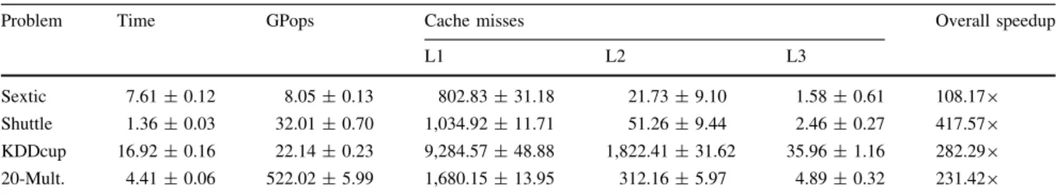
boosted the performance of GP by an average of 11 %. However, most of this gain came from the 20-multiplexer problem whereby a maximal improvement of 28 % was observed. The remaining problems had a much lower performance gain. A reason for this could be that the function set for the multiplexor problem consists of only four simple logical operators. However, loop unrolling provided further significant performance gains over a standard approach to GP. An average overall performance gain of 2609 is now achieved over the standard GP approach with a maximal gain of 4179 for the Shuttle dataset problem.
A second method that can be used to further extend the performance is to reduce the number of GP operators that are called during the evaluation of a candidate solution. Consider for instance a candidate solution which has an add operation followed by a multiplication operator. Instead of each of the operations being executed indepen-dently the two could be combined into a single GP oper-ation. This way three inputs are ‘‘popped’’ off the stack and a single value ‘‘pushed’’ on to the stack. This reduces the number of stack operations by a third. Moreover, only a single GP operator is required and a single loop iterated over instead of two GP operators and two loops. In essence, this is a step closer to a compiled implementation of GP and thus should deliver a performance enhancement.
This methodology could be employed over the entire function set of GP operators. However, this would neces-sitate considerable extra program source code to be written. Thus, for the purposes of demonstration, GP operators which ‘‘double up’’ the arithmetic operators add, subtract, multiply and divide are used producing an extra 16 oper-ators. For the 20-multiplexor problem, the logical boolean operators AND, OR, NAND and NOR are also ‘‘doubled up’’ to also produce an extra 16 operators. Note that these operators are not available to the GP algorithm when constructing candidate solutions. They are simply substi-tuted when interpreting candidate solutions. Algorithm 5 demonstrates a simplified version of the ‘‘MultiplyAdd’’ GP operator.
Table 11 The performance measurements with standard deviation for CPU-based parallel GP with operator loops unrolled three times
Problem Time GPops Cache misses Overall speedup
L1 L2 L3
Sextic 7.61±0.12 8.05±0.13 802.83±31.18 21.73±9.10 1.58±0.61 108.179 Shuttle 1.36±0.03 32.01±0.70 1,034.92±11.71 51.26±9.44 2.46±0.27 417.579 KDDcup 16.92±0.16 22.14±0.23 9,284.57±48.88 1,822.41±31.62 35.96±1.16 282.299 20-Mult. 4.41±0.06 522.02±5.99 1,680.15±13.95 312.16±5.97 4.89±0.32 231.429 Time is measured in seconds, GPops in billions and cache misses are measured in millions
The improvement in execution speed using the ‘‘ dou-bling up’’ of GP operators is demonstrated in Table12. For all problem instances a modest improvement in per-formance has been observed over the results in Table11. In fact, on average a 3 % performance gain was observed with a maximal performance gain of 6 % for the 20-multiplexor problem. This is most likely due to the fact that all the GP operators were ‘‘doubled up’’ for this problem instance. An automated approach could perhaps be used to generate all the ‘‘doubled up’’ GP operators. Also of note is that the cache miss levels are reduced from the results in Table11. This effect is due to the number of stack operations being reduced by the use of ‘‘doubled up’’ GP operators. Thus the final average performance gain achieved by the work presented in this paper is a factor of 267-fold over a standard GP approach. The best performance arose from the Shuttle dataset problem with a 420-fold improvement. The best GPop rate arose from the multiplexor problem with 555 billion GPops. The remaining three problems achieved an average of 21 bil-lion GPops.
8 Comparison with graphics card-based approaches This paper has presented a GP model which provides sig-nificant performance gains using a multi-core CPU. The question now is how does this approach compare to GPU-based implementations of GP. These implementations have also demonstrated significant gains in computational speed over a standard GP approach. Starting with the BlockGP approach (Robilliard et al. 2009) it is possible to compare the results from the sextic regression problem. The BlockGP model achieved a speed of 4.7 billion GPops whilst the Parallel2DStackGP model presented in this paper achieved 8.2 billion GPops. This is nearly twice the speed of the GPU-based approach. However, there are some key differences between the results, the BlockGP approach used a population size of 12,500 whilst the Par-allel2DStackGP approach used only a 1,000 individuals. Moreover, the BlockGP approach has an average tree size of 70 nodes whilst the Parallel2DStackGP approach has only an average of 12.5 nodes.
It is also possible to compare the results from the mul-tiplexor problem with the work by Langdon (2010). With the 37-multiplexor problem Langdon achieved a speed of 256 billion GPops using 32 bit parallelism. The Paral-lel2DStackGP approach achieved a rate of 555 billion GPops also utilising 32 bit parallelism. This is over a twofold improvement on the Langdon approach operating on a graphics card. However, once again the population sizes, the number of generations and the average tree sizes were significantly different.
The two classification problems, the Shuttle and KDD-cup datasets, have been tackled by Cano et al. (2012). Using two GeForce 480 graphics cards an execution time of 0.88 s for the Shuttle dataset and 10.9 seconds for the KDDcup dataset were achieved. The Parallel2DStackGP model presented in this paper achieved 1.351 s for the Shuttle dataset and 22.779 s for the KDDcup dataset. However, the work presented by Cano used only a popu-lation size of 200 individuals evolved over 100 generations
Table 12 The performance gains with standard deviation for CPU-based parallel GP cache exploitive GP approach with ‘‘doubled up’’ GP operators
Problem Time GPops Cache misses Overall speedup
L1 L2 L3
Sextic 7.47±0.10 8.20±0.11 466.08±22.05 21.72±7.08 1.53±1.53 110.249 Shuttle 1.35±0.01 32.2±0.22 988.96±8.94 51.73±1.40 2.48±0.12 420.029 KDDcup 16.44±0.17 22.78±0.23 7247.51±49.53 1455.27±25.95 30.67±0.73 290.519 20-Mult. 4.15±0.07 555.41±9.59 956.12±22.96 181.51±10.26 3.15±0.39 246.229 Time is measured in seconds, GPops in billions and cache misses are measured in millions