NBER WORKING PAPER SERIES
DIAGNOSTIC BUBBLES
Pedro Bordalo
Nicola Gennaioli
Spencer Yongwook Kwon
Andrei Shleifer
Working Paper 25399
http://www.nber.org/papers/w25399
NATIONAL BUREAU OF ECONOMIC RESEARCH
1050 Massachusetts Avenue
Cambridge, MA 02138
December 2018
Gennaioli thanks the European Research Council (GA 647782) for financial support. We are
grateful
to Nicholas Barberis, Lawrence Jin, Josh Schwartzstein, and Alp Simsek for helpful
comments. The views expressed herein are those of the authors and do not necessarily reflect the
views of the National Bureau of Economic Research.
NBER working papers are circulated for discussion and comment purposes. They have not been
peer-reviewed or been subject to the review by the NBER Board of Directors that accompanies
official NBER publications.
© 2018 by Pedro Bordalo, Nicola Gennaioli, Spencer Yongwook Kwon, and Andrei Shleifer. All
rights
reserved. Short sections of text, not to exceed two paragraphs, may be quoted without
explicit permission provided that full credit, including © notice, is given to the source.
Diagnostic Bubbles
Pedro Bordalo, Nicola Gennaioli, Spencer Yongwook Kwon, and Andrei Shleifer
NBER Working Paper No. 25399
December 2018
JEL No. G12,G4
ABSTRACT
We introduce diagnostic expectations into a standard setting of price formation in which investors
learn about the fundamental value of an asset and trade it. We study the interaction of diagnostic
expectations with two well-known mechanisms: learning from prices and speculation (buying for
resale). With diagnostic (but not with rational) expectations, these mechanisms lead to price paths
exhibiting three phases: initial underreaction, followed by overshooting (the bubble), and finally a
crash. With learning from prices, the model generates price extrapolation as a byproduct of fast
moving beliefs about fundamentals,
which lasts only as the bubble builds up. When investors
speculate, even mild diagnostic distortions generate substantial bubbles.
Pedro Bordalo
Saïd Business School
University of Oxford
Park End Street
Oxford, OX1 1HP
United Kingdom
[email protected]
Nicola Gennaioli
Department of Finance
Università Bocconi
Via Roentgen 1
20136 Milan, Italy
[email protected]
Spencer Yongwook Kwon
Department of Economics
Harvard University
1805 Cambridge Street
Cambridge, Mass 02138
United States
[email protected]
Andrei Shleifer
Department of Economics
Harvard University
Littauer Center M-9
Cambridge, MA 02138
and NBER
[email protected]
A Code repository for simulations and graphs is available at
https://github.com/spencerkwon/Bubbleproject_replication
2 1. Introduction
The financial crisis of 2007-2008 has revived academic interest in price bubbles. Shiller (2015) created
a famous graph of home prices in the United States over the course of a century, which shows prices being
relatively stable during most of the 20th century, then doubling over the ten year period after 1996, only to
collapse in the crisis and begin recovering after 2011. There is also growing evidence of speculation such as
buying for resale in the housing market (DeFusco, Nathanson, and Zwick 2018, Mian and Sufi 2018) and of
increasing leverage of both homeowners and financial institutions tied to rapid home price appreciation. The
collapse of the housing bubble is at the heart of every major narrative of the financial crisis and the Great
Recession because it entailed massive losses for homeowners, holders of mortgage backed securities, and financial institutions (Mian and Sufi 2014). Nor is the U.S. experience unique. Leverage expansions and
subsequent crises are often tied to bubbles in housing and other markets (Jorda, Schularick and Taylor 2015).
Despite the revival of academic interest, asset price bubbles remain controversial in finance. Although
economic historians tend to see bubbles as self-evident (Mackay 1841, Bagehot 1873, Galbraith 1954,
Kindleberger 1978, Shiller 2000), Fama (2014) raised the critical question of whether they even exist in the
sense of predictability of future negative returns after prices have increased substantially. Interestingly, since
Smith, Suchanek and Williams (1988), predictably negative returns are commonly found in laboratory
experiments even when markets have finite horizons. Greenwood, Shleifer, and You (2018) address Fama’s
challenge in industry stock return data around the world, and find that although past returns alone are very
noisy indicators of bubbles, other measures of over-pricing do forecast poor returns going forward2.
Early theoretical research has focused on rational price bubbles that do not violate (some definitions
of) market efficiency (e.g., Blanchard and Watson 1982, Tirole 1985, Martin and Ventura 2012), but these
models are not consistent with the available evidence on prices (Giglio, Maggiori, and Stroebel 2016). They
are also rejected by the striking evidence of excessively optimistic investor expectations in bubble episodes
(Case et al. 2012, Greenwood, Shleifer, and You 2018), which also shows up in experimental data (e.g., Haruvy
et al. 2007). Because of such evidence, research has moved to behavioral models of bubbles, which emphasize
2 A closely related literature examines the overpricing of small growth stocks with extremely optimistic analyst forecasts of future growth, and predictably poor returns (Lakonishok et al. 1994, La Porta 1996, Bordalo et al. 2018).
3
factors such as overconfidence and short sales constraints (Scheinkman and Xiong 2003), neglect of entry
(Glaeser et al 2008, Glaeser and Nathanson 2017, Greenwood and Hanson 2014), and extrapolation (e.g.,
Cutler et al. 1990, DeLong et al 1990b, Barsky and DeLong 1993, Hong and Stein 1999, Barberis and Shleifer
2003, Hirshleifer et al. 2015, Glaeser and Nathanson 2017, Barberis et al. 2015, 2018).
Despite substantial advances, many important conceptual questions about price bubbles remain open.
What is the role of innovation, or substantial positive news, in getting bubbles started? Are bubbles driven by
the extrapolation of fundamentals, or of returns themselves? Can price increases become self-reinforcing and
disconnected from fundamental news? And what are the respective roles of optimistic beliefs about fundamental value versus speculation for quick resale in sustaining price growth?
In this paper, we revisit some of these questions starting from a psychologically founded model of
belief formation. We embrace Kindleberger’s (1978) view of bubbles as consisting of three stages. The first
is displacement, meaning a period of good fundamental news, often tied to an economic innovation (see, e.g,
Pastor and Veronesi 2006), that lead to rapid asset price increases. The second and crucial period is the
acceleration of price growth, as price increases themselves encourage buying and further price increases, and
prices reach levels substantially above fundamental values. The third period is the price collapse, as traders
are disappointed and sell the assets. We do not examine leverage and other factors that link the collapses of
bubbles to financial fragility and economic recessions (see, e.g., Gennaioli, Shleifer, and Vishny 2012,
Reinhart and Rogoff 2009, Gennaioli and Shleifer 2018). Our goal is instead to link expectations to the
mechanics of a bubble, including price acceleration and subsequent collapse.
We examine the model of Diagnostic Expectations (see Bordalo, Gennaioli, and Shleifer, hereafter
BGS 2018, Bordalo, Gennaioli, La Porta and Shleifer, hereafter BGLS 2018, and Bordalo, Gennaioli, Ma, and
Shleifer, hereafter BGMS 2018), which relates beliefs to Kahneman and Tversky’s (1972) representativeness
heuristic. Representativeness refers to the notion that, in forming probabilistic assessments, decision makers
put too much weight on outcomes that are likely not in absolute terms, but rather relative to some reference or
baseline level. For example, many people significantly over-estimate the probability that a person’s hair is red when told that the person is Irish. The share of red-haired Irish, at 10%, is a small minority, but red hair is
4
over-estimation of the prevalence of representative types distorts beliefs and accounts for many systematic
errors in probabilistic judgments documented experimentally (Gennaioli and Shleifer 2010). It also delivers a
theory of stereotypes consistent with both field and experimental evidence, including gender stereotypes in
assessments of ability (Bordalo et al. 2018), racial stereotypes in decisions about bail (Arnold, Dobbie and
Yang 2018), and popular beliefs about immigrants (Alesina, Miano, and Stantcheva 2018).
In a market context, diagnostic expectations describe how traders update their beliefs in response to
new information. Under Rational Expectations, the answer to this question is given by the Bayes Rule. Under
Diagnostic Expectations, traders update their beliefs too far in the direction of the states of the world whose objective likelihood has increased the most in light of recent news. After good news, right-tail outcomes
become representative and are overweighed in expectations, while left-tail outcomes become
non-representative and are neglected. This form of over-reaction can lead to overvaluation of financial assets after
good news (BGLS 2018). Here we ask whether it leads to other aspects of the Kindleberger narrative, such as
gradual buildup of prices, extrapolation, acceleration of price growth, and eventual price collapse.
To address these questions, we incorporate diagnostic expectations into a standard finite horizon model
of a market for one asset, in which there is a continuum of investors receiving noisy private information every
period about the termination value of that asset. To capture Kindleberger’s displacement, we assume the asset
is valuable (above the prior) so that traders on average receive good news about fundamentals every period.
Because traders receive different noisy signals, they hold heterogeneous beliefs. Heterogeneity also generates
trading volume, which is an important feature of bubbles (Scheinkman and Xiong 2003, Hong and Stein 2007).
To fix ideas, in Section 2 we describe learning under diagnostic expectations. In Section 3, we present
a model of long horizon investors who learn from prices, and examine how prices respond to a series of good
news. In Section 4, we modify the model to consider short horizon traders whose objective reflects not the
final value of the asset, but next period price. We can thus examine speculation – buying for resale – which is
a central feature of many narratives of the bubbles, including Kindleberger’s. Under Rational Expectations, in
both of these models the average price path increases from the prior to the fundamental value. Whether or not there is learning from prices, there is no overshooting, and hence there are no price bubbles in equilibrium.
5
A model with learning from prices and diagnostic expectations, in contrast, generates some interesting
features of a bubble. As good news come in and prices rise, diagnostic traders act more aggressively on their
private signals, which makes prices more informative than under the rational benchmark. As a consequence,
traders react even more aggressively to price signals, which quickly swamp the less informative private ones.
Prices not only exceed fundamental values in equilibrium, but also accelerate as the bubble develops. In fact,
it looks like investors are extrapolating price trends, even though they are not. Instead, recent price increases lead traders to upgrade (too much) their expectations of fundamental value, and thus of the future price.
Despite some plausible intuitions, the model in Section 3 does not deliver wild prices because equilibrium
prices are still tethered to eventual liquidation values.
In Section 4, we introduce speculation by having traders optimize relative to their beliefs of the next
period price rather than the eventual liquidation value of the asset. Unlike previous models of speculation, such
as Harrison and Kreps (1978) and Scheinkman and Xiong (2003), we do not need to assume short sale
constraints. This modification has dramatic consequences. Even without learning from prices, traders can drive
prices extremely high, because speculation compounds overreaction: traders are not only too optimistic about
fundamentals, they also exaggerate the possibility of reselling the asset to over-reacting traders in the future.
Following a beauty context logic, a trader who believes that the asset is the next Google thinks that future
diagnostic traders will receive extremely positive signals and will thus be even more optimistic about the asset.
The expectation of reselling the asset to very bullish traders further inflates the price today. Eventually, as the
terminal date approaches, the opportunities for resale become scarcer and the bubble collapses.
Along with diagnostic expectations, speculation emerges as a central feature of price bubbles, at least
in terms of the three Kindleberger phases. When combined with learning from prices, speculation disconnects
expectations of fundamentals from expectations of price increases. Even a small deviation from rationality in
6
2. Learning from Good Shocks and the Dynamics of Diagnostic Expectations
Our basic setup is as follows. Traders learn about the value of a new asset over a finite number of
periods 𝑡𝑡= 0, … ,𝑇𝑇. The asset yields a payoff 𝑉𝑉 drawn from a normal distribution with mean 0 and variance
𝜎𝜎𝑉𝑉2 at 𝑡𝑡= 0 but is only revealed at the terminal date 𝑇𝑇. In line with Kindelberger’s (1978) description of a positive displacement as the trigger of bubble episodes, we focus on the case of a valuable innovation, 𝑉𝑉 > 0. In each period 𝑡𝑡, each trader 𝑖𝑖 (in measure one) receives a private signal 𝑠𝑠𝑖𝑖𝑖𝑖 =𝑉𝑉+𝜖𝜖𝑖𝑖𝑖𝑖 of the asset’s value. Noise 𝜖𝜖𝑖𝑖𝑖𝑖 is i.i.d. across traders and over time, and normally distributed with mean zero and variance 𝜎𝜎𝜖𝜖2. Because the new asset is valuable, 𝑉𝑉 > 0, traders are repeatedly exposed to good news, in that signals are on average positive relative to their priors, capturing the initial displacement. Moreover, the assumption of
dispersed information generates variation in expectations and helps account for trading.
In this Section, we do not consider trading, and describe instead how Diagnostic Expectations about
fundamentals evolve solely based on the arrival of noisy private signals over time. This is useful for two
reasons. First, in this setting with learning and dispersed information, Diagnostic Expectations behave
differently than in prior finance applications (BGS 2018, BGLS 2018). Second, by separately characterizing
the dynamics of expectations about fundamentals, we can better understand their interaction with market forces
such as trading, learning from prices, and speculation, which we introduce in Sections 3 and 4.
A rational trader observing a history of signals (𝑠𝑠𝑖𝑖1, … ,𝑠𝑠𝑖𝑖𝑖𝑖) forms an expectation about 𝑉𝑉 given by:
𝔼𝔼𝑖𝑖𝑖𝑖(𝑉𝑉) =𝜋𝜋𝑖𝑖∑ 𝑠𝑠𝑖𝑖𝑖𝑖 𝑖𝑖 𝑖𝑖=1
𝑡𝑡 ,
where 𝜋𝜋𝑖𝑖 ≡ 𝑖𝑖 𝜎𝜎⁄ 𝜖𝜖2
𝑖𝑖 𝜎𝜎⁄ +1 𝜎𝜎𝜖𝜖2 ⁄ 𝑉𝑉2 is the signal to noise ratio. Prices will be driven by the consensus expectation, given by
� 𝔼𝔼𝑖𝑖𝑖𝑖(𝑉𝑉)𝑑𝑑𝑖𝑖=𝜋𝜋𝑖𝑖𝑉𝑉. (1)
The consensus expectation of rational traders exhibits two important properties. First, it is always
below the rational benchmark because 𝜋𝜋𝑖𝑖≤1. Rational traders discount their noisy signals, which implies that average information, always equal to 𝑉𝑉, is also discounted. Second, the consensus expectation gradually
7
improves over time, because the signal to noise ratio 𝜋𝜋𝑖𝑖 rises, in a concave way, toward one. As the trader sees more and more signals, his uncertainty falls, inducing him to weigh his evidence more heavily.
As in rational inattention or noisy information models (Woodford 2003), optimal information
processing by individuals who observe noisy signals creates sluggishness in consensus expectations. This sluggishness is central in thinking about price formation in rational expectations models. Indeed, as we show
in Sections 3 and 4, rational updating implies that the price of the asset monotonically converges to
fundamental value from below, just as consensus expectations do.
Consider now updating under Diagnostic Expectations (DE) in a model of beliefs formation.3 In an
intertemporal setting like the current one, this model captures the idea that, when forming beliefs about the
future, investors overweight the probability of events that have become more likely in light of recent news.
For instance, after observing a period of positive earnings growth, DE overweight the probability that the firm
may be the next Google. Even though this event is highly unlikely in absolute terms, it has become more likely
in light of the strong earnings growth. As a consequence, the perceived probability of such an event is inflated.
As shown in BGS (2018), if the random variable 𝑋𝑋𝑖𝑖+1 is conditionally normal, the diagnostic
distribution of beliefs is also normal.4 Furthermore, if 𝔼𝔼
𝑠𝑠(𝑋𝑋𝑖𝑖+1) is the rational expectation at time 𝑠𝑠, then the diagnostic expectation at time 𝑡𝑡 is:
𝔼𝔼𝑖𝑖𝜃𝜃(𝑋𝑋𝑖𝑖+1) =𝔼𝔼𝑖𝑖−𝑘𝑘(𝑋𝑋𝑖𝑖+1) + (1 +𝜃𝜃)[𝔼𝔼𝑖𝑖(𝑋𝑋𝑖𝑖+1)− 𝔼𝔼𝑖𝑖−𝑘𝑘(𝑋𝑋𝑖𝑖+1)], (2) DE are forward looking: they update in the correct direction and nest rational expectations as a special
case for 𝜃𝜃= 0. Crucially, however, DE overreact to information by exaggerating the difference between
current conditions 𝔼𝔼𝑖𝑖(𝑋𝑋𝑖𝑖+1) and normal conditions 𝔼𝔼𝑖𝑖−𝑘𝑘(𝑋𝑋𝑖𝑖+1) by a factor of (1 +𝜃𝜃). As good news arrives, the right tail of 𝑋𝑋𝑖𝑖+1 becomes fatter; while still unlikely, this right tail is very representative because its prior
3According to Kahneman and Tversky (1972), the reliance on representativeness as a proxy for likelihood is a central
feature of probabilistic judgments. An outcome “is representative of a class if it’s very diagnostic”, that is, if its “relative frequency is much higher in that class than in the relevant reference class” (Tversky and Kahneman 1983).
4 Following BGS (2018), in a Markov process with density 𝑓𝑓(𝑋𝑋
𝑖𝑖+1|𝑋𝑋𝑖𝑖), after a particular current state 𝑋𝑋�𝑖𝑖 is realized and
in light of the past expectation for the current state 𝔼𝔼𝑖𝑖−𝑘𝑘(𝑋𝑋𝑖𝑖), the distorted distribution is equal to: 𝑓𝑓𝜃𝜃(𝑋𝑋
𝑖𝑖+1|𝑋𝑋𝑖𝑖) =𝑓𝑓(𝑋𝑋𝑖𝑖+1|𝑋𝑋𝑖𝑖)� 𝑓𝑓�𝑋𝑋𝑖𝑖+1|𝑋𝑋�𝑖𝑖�
𝑓𝑓�𝑋𝑋𝑖𝑖+1|𝔼𝔼𝑖𝑖−𝑘𝑘(𝑋𝑋𝑖𝑖)�� 𝜃𝜃
𝑍𝑍𝑖𝑖,
where both the target 𝑓𝑓�𝑋𝑋𝑖𝑖+1|𝑋𝑋�𝑖𝑖� and reference distribution 𝑓𝑓�𝑋𝑋𝑖𝑖+1|𝔼𝔼𝑖𝑖−𝑘𝑘(𝑋𝑋𝑖𝑖)� have equal variance. Roughly speaking, beliefs overweigh states that have become more likely in light of the surprise 𝑋𝑋�𝑖𝑖− 𝔼𝔼𝑖𝑖−𝑘𝑘(𝑋𝑋𝑖𝑖) relative to 𝑘𝑘 periods ago.
8
probability was so low. As a result, investors overweight the right tail and neglect the risk in the left tail. For
normal distributions, this reweighting results in an excessive rightward shift of beliefs.
In Equation (2), lag 𝑘𝑘 defines which recent news investors over-react to. For 𝑘𝑘 = 1, investors only overreact to news received in the current period, so after one period past good news are immediately perceived
as normal. For 𝑘𝑘 > 1, the investor over-reacts to the last 𝑘𝑘 pieces of news. This captures a realistic sluggishness in the perception of normal conditions: new evidence becomes normal only after enough time has
passed. Put differently, the investor observing a sequence of good news takes a while to adapt to them.
BGLS (2018) show that in a setting where traders learn from homogeneous information, diagnostic
expectations obtained from Equation (2) account well for the link between listed firms’ performance and equity
analysts’ expectations of their future earnings growth, as well as, crucially, for the link between expectations
and the predictability of their stock returns. They estimate the model and find that, with quarterly data, 𝜃𝜃 ≈1 and 𝑘𝑘 ≈3 years. A similar value of 𝜃𝜃 has been estimated using expectations of credit spreads by BGS, and
using macroeconomic forecasts by BGMS. Later we use 𝑘𝑘 ≈3 years in our simulation exercises.
The current model, relative to earlier finance applications of DE, we introduce two new ingredients.
First, each trader observes a different noisy signal of the truth 𝑉𝑉. Second, the state 𝑉𝑉 does not change over time, reflecting learning about, say, the potential of a new technological innovation. We next show that under
these two assumptions DE generate rich dynamics that look promising for studying bubble episodes.
Given the heterogeneity of information at time 𝑡𝑡 each trader 𝑖𝑖 has a different diagnostic expectation
𝔼𝔼𝑖𝑖𝑖𝑖𝜃𝜃(𝑉𝑉). As before, we focus on the consensus diagnostic expectation. This is given by:
� 𝔼𝔼𝑖𝑖𝑖𝑖𝜃𝜃(𝑉𝑉)𝑑𝑑𝑖𝑖=� (1 +𝜃𝜃)𝜋𝜋𝑖𝑖𝑉𝑉 𝑓𝑓𝑓𝑓𝑓𝑓 𝑡𝑡 ≤ 𝑘𝑘 [𝜋𝜋𝑖𝑖+𝜃𝜃(𝜋𝜋𝑖𝑖− 𝜋𝜋𝑖𝑖−𝑘𝑘)]𝑉𝑉 𝑓𝑓𝑓𝑓𝑓𝑓 𝑡𝑡>𝑘𝑘
. (3)
Equation (3) implies that, under DE, consensus expectations exhibit boom bust dynamics.
Proposition 1If 𝜃𝜃 ∈ �1
𝑘𝑘 𝜎𝜎𝜖𝜖2
𝜎𝜎𝑣𝑣2,
𝜎𝜎𝜖𝜖2
𝜎𝜎𝑣𝑣2�, the consensus diagnostic expectation 𝔼𝔼𝑖𝑖
𝜃𝜃(𝑉𝑉) exhibits three phases:
9
2) Bust: 𝔼𝔼𝑖𝑖𝜃𝜃(𝑉𝑉) drops from 𝑡𝑡=𝑘𝑘+ 1 to 𝑡𝑡∗, reaching its through 𝔼𝔼𝑖𝑖𝜃𝜃∗(𝑉𝑉) <𝑉𝑉.
3) Recovery: 𝔼𝔼𝑖𝑖𝜃𝜃(𝑉𝑉) gradually recovers for 𝑡𝑡>𝑡𝑡∗, asymptotically converging to the fundamental 𝑉𝑉.
In a noisy environment, adding a modicum of overreaction 𝜃𝜃 to recent signals upsets the monotone
convergence of rational expectation, yielding rich beliefs dynamics. Early on, consensus opinion under-reacts
to the fundamental displacement, 𝔼𝔼𝑖𝑖𝜃𝜃(𝑉𝑉) <𝑉𝑉, so that in this range the behavior of DE is qualitatively similar to rational learning. Because diagnostic traders are forward looking, they discount the noise in their signals.
Initially, when uncertainty about V is large, this discounting is sufficiently strong that it counteracts the
tendency of each individual to overreact (as long as overreaction is moderate, 𝜃𝜃<𝜎𝜎𝜖𝜖2
𝜎𝜎𝑣𝑣2). As a result, in early
stages, consensus beliefs about V improve sluggishly, gradually incorporating the good signals of traders.
The possibility that in a noisy environment individual over-reaction is consistent with sluggishness of
consensus expectations is not just theoretical. BGMS (2018) document this phenomenon in professional
forecasts of macroeconomic variables. When expectations are heterogeneous, as is empirically the case,
information contained in the average is lost, creating apparent under-reaction.
As traders receive good signals, however, they grow more confident about the value of the asset. As
a result, they incorporate their signals more aggressively into their beliefs. At some point, their signal to noise
ratio 𝜋𝜋𝑖𝑖 becomes sufficiently high that, for a given amount of diagnosticity 𝜃𝜃 we have: (1 +𝜃𝜃)𝜋𝜋𝑖𝑖 > 1.
Consensus under-reaction now turns to overreaction. Displacement causes traders to be so confident
that beliefs overshoot the fundamental, 𝔼𝔼𝑖𝑖𝜃𝜃(𝑉𝑉) >𝑉𝑉. Overshooting of fundamentals stands in stark contrast not only to the rational benchmark but also to any model of mis-specified learning in which beliefs are a convex
combination of priors and new information, including overconfidence (Daniel, Hirshleifer and Subrahmanyam
1998).5 This distinctive feature reflects the fact that diagnostic expectations generate disproportional and
asymmetric weight on tail events: if traders focus on the right tail and neglect the left tail, then in some sense
5 Overconfidence is a different form of over-reaction to private news in which traders exaggerate the precision of their private signals. It implies an inflated signal to noise ratio relative to rational expectations, but still be below 1. This generates a price path lying above the rational benchmark, but never overshooting or exhibiting a boom-bust path.
10
“the sky is the limit”: sufficiently many good signals about 𝑉𝑉 bring to mind stratospheric values, each fast growing firm is believed to be a new Google, and trees are expected to grow to the sky. This result is in line with the standard narrative of bubbles, in which the initial displacement leads investors to believe in a
“paradigm shift” capturing the most optimistic scenarios that could result from the innovation.6
Beliefs revert after 𝑘𝑘 periods, when over-reaction to early signals wanes. After a while, traders view these signals as normal and focus on the information contained in the new, most recent, signals. Because these
signals have a smaller and smaller incremental value (𝑉𝑉 is finite), they cannot sustain the exorbitant optimism of the boom. As a result, optimism in beliefs starts deflating. The bust here is due not to bad news, but to the
declining pace at which good news arrive, which causes optimism to run out of steam. After the bust, when
expectations reach their trough and get close to rational beliefs, over-reaction to good news is negligible
(because good news are minor), and the consensus converges to 𝑉𝑉 from below.
In sum, by introducing some over-reaction to recent news in an otherwise standard noisy information
model, diagnostic expectations can account for initial rigidity of consensus expectations, delayed over-reaction
of beliefs to fundamental news, and subsequent reversals as dramatic good news stop coming. This mechanism
seems promising for thinking about bubbles. Insofar as prices reflect consensus beliefs, diagnostic expectations
may account for sluggish boom bust price dynamics that cannot be obtained under rationality. Still, other
features of this simple formulation are hard to reconcile with bubbles. First, expectations of fundamentals in
Equation (3) improve in a concave way, which is hard to square with the observed convex price paths during
bubbles (Greenwood, Shleifer, and Yang 2018). Second, for realistic parameter values over-optimism about
fundamentals is small relative to the price inflation observed in bubble episodes. Using 𝜃𝜃= 1 as estimated using expectations of earnings growth (BGLS 2018), and of macroeconomic time series (BGMS 2018),
suggests that valuation at the peak is bounded above by 2𝑉𝑉. In some historical episodes, such as the internet bubble, prices reached multiple times the plausible measures of fundamentals.
To address these challenges, we next combine diagnostic expectations about fundamentals with two
standard mechanisms that do not yield the three phases of bubbles in rational models: learning from prices and
6 In Pastor and Veronesi (2009), a successful innovation is not initially overpriced, but instead becomes central enough to
11
speculation. We show that combining these standard market mechanisms with a modicum of diagnosticity
about fundamentals is able to reproduce key features of bubble episodes, including convex price paths and
strongly inflated prices. Prices growth becomes disconnected from growth in fundamentals.
3. Diagnostic Learning from Prices
We now analyze trading when traders learn not only from private signals, but also from market prices. This is an important feature of real world markets, enabling traders to extract from price changes the
information that other traders have about fundamentals. Starting with Grossman (1976) and Grossman and
Stiglitz (1980), learning from prices plays an important role in formal analyses of rational expectations
equilibria in financial markets. Here we study its consequences under diagnostic expectations.
The market setting is as follows. At each 𝑡𝑡= 0,1 …, traders exchange the asset and determine its price. They learn about the fundamental 𝑉𝑉 from current and past private signals as well as from all prices observed up to the last period.7 Traders are risk averse with CARA utility 𝑢𝑢(𝑐𝑐) =−𝑒𝑒−𝛾𝛾𝛾𝛾, and they have long horizons,
in that they value the asset by their assessment of its fundamental value 𝑉𝑉. There is no time discounting. To determine the demand for the asset at time 𝑡𝑡, suppose that trader 𝑖𝑖 believes that 𝑉𝑉 is normally distributed with mean 𝔼𝔼𝑖𝑖𝑖𝑖𝜃𝜃(𝑉𝑉) and variance 𝜎𝜎𝑖𝑖2(𝑉𝑉), where 𝜃𝜃 denotes diagnostic expectations.8 With exponential
utility and normal beliefs, his preferences are described in terms of mean and variance. Trader i’s demand 𝐷𝐷𝑖𝑖𝑖𝑖 of the asset maximizes the mean-variance objective function:
𝐷𝐷𝑖𝑖𝑖𝑖 = max𝐷𝐷�
𝑖𝑖𝑖𝑖 �𝔼𝔼𝑖𝑖𝑖𝑖
𝜃𝜃(𝑉𝑉)− 𝑝𝑝
𝑖𝑖�𝐷𝐷�𝑖𝑖𝑖𝑖−𝛾𝛾2 𝜎𝜎𝑖𝑖2(𝑉𝑉)𝐷𝐷�𝑖𝑖𝑖𝑖2,
where 𝛾𝛾 captures risk aversion. Trader 𝑖𝑖’s demand 𝐷𝐷𝑖𝑖𝑖𝑖 is then given by:
7 If investors learn also from the current price, the equilibrium may fail to exist for 𝑡𝑡>𝑘𝑘. We thus focus on learning from past prices, which guarantees existence, but the models behave very similarly when equilibrium exists. To study speculation, because we set 𝑘𝑘 to be high, existence is guaranteed and so we allow investors to learn from the current price.
8 As we discussed in Section 2, diagnostic beliefs are normal. This is shown in the appendix, where we also show that the
12
𝐷𝐷𝑖𝑖𝑖𝑖 =𝔼𝔼𝑖𝑖𝑖𝑖
𝜃𝜃(𝑉𝑉)− 𝑝𝑝 𝑖𝑖
𝛾𝛾𝜎𝜎𝑖𝑖2(𝑉𝑉) , (4) Intuitively, demand increases in the difference between the trader’s valuation and the market price.
To make learning from prices non-degenerate, we follow the literature and assume that that the supply
𝑆𝑆𝑖𝑖 of the asset is random, i.i.d. normal with mean zero and variance 𝜎𝜎𝑆𝑆2 (without supply shocks 𝑉𝑉 is learned in one period). The classical justification here is the presence of noise or liquidity traders who demand/supply
the assets for non-fundamental reasons (Black 1986, Grossman and Miler 1988, DeLong et al. 1990a). The
implication is that price is no longer fully revealing: high price today may be due either to a low unobserved
supply 𝑆𝑆𝑖𝑖 shock or to a high average private signal 𝑉𝑉.
By aggregating individual demands in Equation (4) and by equating to supply we find:
𝑝𝑝𝑖𝑖 =� 𝔼𝔼𝑖𝑖𝑖𝑖𝜃𝜃(𝑉𝑉)𝑑𝑑𝑖𝑖 − 𝛾𝛾𝜎𝜎𝑖𝑖2(𝑉𝑉)𝑆𝑆𝑖𝑖. (5) To solve for the equilibrium in Equation (5), we must compute the diagnostic consensus expectation
at time 𝑡𝑡, recognizing that it depends both private signals and past prices. Because DE are forward looking, it is possible to amend the consensus beliefs in Equation (3) to reflect diagnostic learning from prices. As in
rational expectations models (Grossman and Stiglitz 1980), we first conjecture that, at each time 𝑡𝑡, price is a
linear function of the state variables of the economy, which include the fundamental 𝑉𝑉. Second, we assume
that traders use this linear rule to make inferences about 𝑉𝑉 in light of the current and past prices. Third, we determine at each time 𝑡𝑡 the coefficients of the pricing function that equilibrate demand and supply, so that the resulting rule yields the equilibrium price.
Denote by 𝔼𝔼(𝑉𝑉|𝑃𝑃𝑖𝑖) the rational expectation of 𝑉𝑉 based solely on the history of prices up to 𝑡𝑡, formally
𝑃𝑃𝑖𝑖 ≡(𝑝𝑝1, … ,𝑝𝑝𝑖𝑖−1). Then, our conjectured pricing rule takes the form:9
𝑝𝑝𝑖𝑖 =𝑎𝑎1𝑖𝑖+𝑎𝑎2𝑖𝑖𝔼𝔼(𝑉𝑉|𝑃𝑃𝑖𝑖) +𝑎𝑎3𝑖𝑖𝔼𝔼(𝑉𝑉|𝑃𝑃𝑖𝑖−𝑘𝑘) +𝑏𝑏𝑖𝑖�𝑉𝑉 −𝑏𝑏𝑐𝑐𝑖𝑖
𝑖𝑖𝑆𝑆𝑖𝑖�. (6)
9 The price could equivalently be assumed to be linear in the diagnostic expectation 𝔼𝔼𝜃𝜃(𝑉𝑉|𝑃𝑃
𝑖𝑖,𝑠𝑠𝑖𝑖1=⋯=𝑠𝑠𝑖𝑖𝑖𝑖= 0) held by
13
Equation (6) is reminiscent of rational expectations analyses. The current price reflects consensus expectations
derived from all prices up to date 𝑡𝑡, as well as the average private signal. Because diagnostic expectations combine current and lagged rational forecasts, the lagged forecast is also added as a state variable.
To solve for the diagnostic expectations equilibrium (DEE), we must find the coefficients (𝑎𝑎1𝑖𝑖,𝑎𝑎2𝑖𝑖,𝑎𝑎3𝑖𝑖,𝑏𝑏𝑖𝑖,𝑐𝑐𝑖𝑖)𝑖𝑖≥1 that equate supply with demand when traders make diagnostic inferences from prices. We now sketch the logic of the result, and leave a fuller account to the proof in Appendix A.
First, consider how traders learn in light of the pricing rule. Because diagnostic traders over-react to
news, they over-react also to the shared news coming from prices. To compute the diagnostic expectations
with learning from prices, we proceed in two steps. We compute the rational expectations when prices are
generated by Equation (6), and then apply the diagnostic transformation of Equation (2).10
The rational news conveyed by price at time 𝑓𝑓 is captured by the term 𝑝𝑝𝑖𝑖− 𝑎𝑎1𝑖𝑖− 𝑎𝑎2𝑖𝑖𝔼𝔼(𝑉𝑉|𝑃𝑃𝑖𝑖)−
𝑎𝑎3𝑖𝑖𝔼𝔼(𝑉𝑉|𝑃𝑃𝑖𝑖−𝑘𝑘) as well as by the coefficients 𝑏𝑏𝑖𝑖 and 𝑐𝑐𝑖𝑖, which are known by all (in equilibrium). That is, observing 𝑝𝑝𝑖𝑖 effectively endows all traders with the following unbiased public signal of 𝑉𝑉:
𝑠𝑠𝑖𝑖𝑝𝑝=𝑉𝑉 − �𝑐𝑐𝑏𝑏𝑖𝑖
𝑖𝑖� 𝑆𝑆𝑖𝑖. (7) The variance of the signal, which is the inverse of its precision, is equal to (𝑐𝑐𝑖𝑖/𝑏𝑏𝑖𝑖)2𝜎𝜎𝑆𝑆2. Intuitively, the price is more informative when it is more sensitive to the persistent fundamental than to the transient supply shock,
namely when 𝑐𝑐𝑖𝑖/𝑏𝑏𝑖𝑖 is lower. This price sensitivity is an endogenous part of the equilibrium, and later we characterize it in terms of primitives.
Since private and public signals 𝑠𝑠𝑖𝑖𝑖𝑖 and 𝑠𝑠𝑖𝑖𝑝𝑝 are normally distributed, conditional on a history of signals
�𝑠𝑠𝑖𝑖1, …𝑠𝑠𝑖𝑖𝑖𝑖,𝑠𝑠1𝑝𝑝, …𝑠𝑠𝑖𝑖𝑝𝑝�, a rational trader’s beliefs about 𝑉𝑉 are normal with mean:
𝔼𝔼𝑖𝑖,𝑖𝑖(𝑉𝑉) =𝑠𝑠̅𝑖𝑖,𝑖𝑖𝑧𝑧𝑖𝑖+𝔼𝔼(𝑉𝑉|𝑃𝑃𝑖𝑖)(1− 𝑧𝑧𝑖𝑖), (9)
10In the appendix we show that the diagnostic expectations so obtained are equivalent to those obtained by applying the
14
The rational inference combines the private signals with the price signals embodied in 𝔼𝔼(𝑉𝑉|𝑃𝑃𝑖𝑖). The weight 𝑧𝑧𝑖𝑖 attached to the private signals is given by:11
𝑧𝑧𝑖𝑖 =σ𝑡𝑡 ϵ 2� 𝑡𝑡 σϵ2+ 1 𝜎𝜎𝑝𝑝2,𝑖𝑖(𝑉𝑉)� −1 , (10) where 𝜎𝜎𝑝𝑝2,𝑖𝑖(𝑉𝑉) is the variance of the fundamental conditional only on prices. The weight 𝑧𝑧𝑖𝑖 attached to private signals is higher when the informativeness of prices is low (when 𝜎𝜎𝑝𝑝2,𝑖𝑖(𝑉𝑉) is high).
To compute diagnostic consensus beliefs, we need to: i) compute diagnostic beliefs by transforming
rational beliefs in Equation (10) according to Equation (2), and ii) aggregate the resulting beliefs into the
consensus. The implied consensus dynamics works as follows:
� 𝔼𝔼𝑖𝑖𝑖𝑖𝜃𝜃(𝑉𝑉)𝑑𝑑𝑖𝑖=� (1 +𝜃𝜃)[(1− 𝑧𝑧𝑖𝑖)𝔼𝔼(𝑉𝑉|𝑃𝑃𝑖𝑖) +𝑉𝑉𝑧𝑧𝑖𝑖] 𝑓𝑓𝑓𝑓𝑓𝑓 𝑡𝑡 ≤ 𝑘𝑘 (1 +𝜃𝜃)(1− 𝑧𝑧𝑖𝑖)𝔼𝔼(𝑉𝑉|𝑃𝑃𝑖𝑖)− 𝜃𝜃(1− 𝑧𝑧𝑖𝑖−𝑘𝑘)𝔼𝔼(𝑉𝑉|𝑃𝑃𝑖𝑖−𝑘𝑘) + [(1 +𝜃𝜃)𝑧𝑧𝑖𝑖− 𝜃𝜃𝑧𝑧𝑖𝑖−𝑘𝑘]𝑉𝑉 𝑓𝑓𝑓𝑓𝑓𝑓 𝑡𝑡>𝑘𝑘 .
There are two important messages. First, diagnostic expectations exaggerate the information revealed
by prices, not only private information. This exaggeration comes from the amplification (1 +𝜃𝜃) of the impact of the current price-based estimate 𝔼𝔼(𝑉𝑉|𝑃𝑃𝑖𝑖), and from the reversal of past price inferences 𝔼𝔼(𝑉𝑉|𝑃𝑃𝑖𝑖−𝑘𝑘). This is another difference from overconfidence, in which public information – including that coming from prices – is
underweighted. Because a price increase says that positive information about fundamentals is dispersed in the
economy, it renders the right tail representative, causing overreaction in beliefs. Second, if prices become very
informative over time, the weight 𝑧𝑧𝑖𝑖 attached to private signals falls and the weight attached to prices increases. The effects of information dispersion may thus subside, and the dynamics of beliefs may be very different
from what we saw in Section 2.
3.1 The Boom Phase
11The variance of 𝑉𝑉 is equal to 𝜎𝜎
𝑖𝑖2(𝑉𝑉) =�σ𝑖𝑖 ϵ 2+𝜎𝜎 1
𝑝𝑝,𝑖𝑖2 (𝑉𝑉)� −1
. 𝜎𝜎𝑝𝑝2,𝑖𝑖(𝑉𝑉) decreases in the precision of the public signals observed up to 𝑡𝑡. See the appendix for details.
15
To assess whether learning from prices significantly affects beliefs and prices, we need to solve for
the coefficient of price informativeness 𝑐𝑐𝑖𝑖/𝑏𝑏𝑖𝑖. It may in fact be that diagnosticity reduces price
informativeness, moderating overreaction to price signals. We need to find a fixed point at which consensus beliefs are consistent with market equilibrium in Equation (5). Here the key result comes from considering the
equilibrium for the boom phase of the bubble, 𝑡𝑡 ≤ 𝑘𝑘.
Proposition 2With learning from prices and 𝑡𝑡 ≤ 𝑘𝑘, the average consensus belief about 𝑉𝑉 is higher than the average consensus belief formed when investors learn from private information alone. The precision of the equilibrium price signal increases over time as:
𝑏𝑏𝑖𝑖
𝑐𝑐𝑖𝑖 =� 1 +𝜃𝜃
𝛾𝛾σϵ2 � 𝑡𝑡, (11)
and the average equilibrium price path (for 𝑆𝑆1=𝑆𝑆2=⋯=𝑆𝑆𝑖𝑖 = 0) is given by:
𝑝𝑝𝑖𝑖 = (1 +𝜃𝜃) ⎣ ⎢ ⎢ ⎢ ⎡ 𝑡𝑡 σϵ2+� 1 +𝜃𝜃 σ𝑆𝑆σϵ2� 2𝑡𝑡(𝑡𝑡 −1)(2𝑡𝑡 −1) 6 𝑡𝑡 σϵ2+ 1σV2+� 1 +𝜃𝜃 σ𝑆𝑆σϵ2� 2𝑡𝑡(𝑡𝑡 −1)(2𝑡𝑡 −1) 6 ⎦⎥ ⎥ ⎥ ⎤ 𝑉𝑉. (12)
As in the consensus expectations described in Section 2, the equilibrium price grows in the boom phase
𝑡𝑡 ≤ 𝑘𝑘, before investors adapt to the displacement. The price in Equation (12) increases over time. If 𝜃𝜃 in in the
range of Proposition 1, the price starts below the fundamental 𝑉𝑉. This initial under-reaction is due to the same reason that consensus beliefs underreact: traders discount the noise in their signals, so the good news they on
average receive is not incorporated into prices.
As time goes by, the price increases due to two forces. First, as traders accumulate private signals,
they gain confidence about the innovation and revise their beliefs upward. This effect is captured by the term
𝑡𝑡/σϵ2 in Equation (12). Second, the observation of prices provides on average additional good news about displacement and that makes all traders more confident at the same time. As a result, the consensus estimate
of 𝑉𝑉 increases relative to the case in which only private signals are observed, and the price booms. The effect of learning from prices is captured by the second term in the numerator of Equation (12). At some point,
16
How does diagnosticity interact with learning from prices? And how does learning from prices
contribute to the price path? Equation (11) answers the first question. Stronger diagnosticity 𝜃𝜃 increases the informativeness of prices. When 𝜃𝜃 is higher, investors are aggressive both in revising their beliefs and in
trading on the basis of their private signals. Because these signals are informative about 𝑉𝑉, price
informativeness increases. In turn, greater price informativeness implies that diagnostic traders over-react
faster to the price signals, which implies that the bubble arises earlier. Unlike non-fundamental based
behavioral biases, such as mechanical extrapolation, which disconnect prices from fundamentals, diagnostic
expectations exaggerate this link, creating faster and accelerating overreaction to the initial displacement.
To see how learning from prices influences the price path, consider again Equation (11). It says that,
for a given 𝜃𝜃, the price signal becomes more informative over time. As the i.i.d. supply shocks average out over time, a path of consistent price increases is highly informative of good fundamentals. Consequently,
learning from prices progressively gains ground, and swamps private signals as prices rise up to the peak of
the bubble. As shown in Equation (12) the precision of price signals grows with the cubic power of 𝑡𝑡, which eventually swamps the linear precision of private signals, 𝑡𝑡/σϵ2. This has the following implication.
Proposition 3With learning from prices, there exists a 𝜎𝜎𝑉𝑉2∗> 0 such that for 𝜎𝜎𝑉𝑉2<𝜎𝜎𝑉𝑉2∗ there exists a 𝑡𝑡∗> 0 such the average price path is convex for 𝑡𝑡<𝑡𝑡∗ and concave for 𝑡𝑡 ∈(𝑡𝑡∗,𝑘𝑘). When the supply shocks are so volatile ( σ𝑆𝑆→ ∞) that prices convey no information, the price path is concave: 𝜎𝜎𝑉𝑉2∗→0.
When fundamental displacement is sufficiently large (𝜎𝜎𝑉𝑉2 is low enough), learning from prices
generates a price path that is initially convex and then slows down as the bubble reaches its peak. This occurs
because all traders, regardless of their private signals, aggressively infer fundamentals from the common price
signal, so the price informativeness increases at first. After sufficient information has been incorporated into
expectations and prices, the value of additional signals diminishes, which causes a price growth slowdown.
Under rational expectations, learning from prices would also coordinate traders’ beliefs and generate
convexity in prices, but not lead to overvaluation. In contrast, under diagnostic expectations convex price
growth eventually overshoots the fundamentals, creating a bubble. In this respect, with learning from prices,
17
continues and as the price increases, traders make strong inferences and push the price even higher, generating
a convex price increase and eventually an overvaluation. Allowing for learning from prices thus remedies the
first shortcoming of the model of Section 2: it creates the convex price paths typical of real world bubbles.
3.2 Model Simulation: Boom, Bust and Price Extrapolation
To explore the entire path of the bubble, we resort to simulations, because the model cannot be
analytically solved for 𝑡𝑡>𝑘𝑘. This analysis shows that diagnostic expectations can produce the boom and bust phases of bubbles and the dynamics of investor disagreement (and hence trading). Most importantly, diagnostic
expectations can endogenously produce extrapolative expectations of prices, but in a way that distinguishes
them from adaptive expectations or from alternative formulations (Hong and Stein 1999, Glaeser and
Nathanson 2017). The predictions may also suggest how to detect bubbles in the data.
We now describe our choice of parameters. We normalize 𝑉𝑉 to 1. To capture that displacement is a fairly rare event, we assume 𝜎𝜎𝑉𝑉= 0.5, so 𝑉𝑉 is two standard deviations away from the mean. The dispersion of trader’s private signals is set at 𝜎𝜎𝜖𝜖 = 12.5, which is in the ballpark of what we estimated from the quarterly dispersion of professional forecasts (BGMS 2018).12 We set 𝜃𝜃 = 0.8, in line with the quarterly estimates from
macroeconomic and financial survey data. For the model without speculation, we take a time period to be a
quarter, set the sluggishness of diagnostic beliefs at 𝑘𝑘 = 12 (in line with the estimates from BGLS 2018) and run the model for 𝑇𝑇= 24 periods, i.e. 6 years. We set the volatility of supply shocks at 𝜎𝜎𝑆𝑆= 0.3.
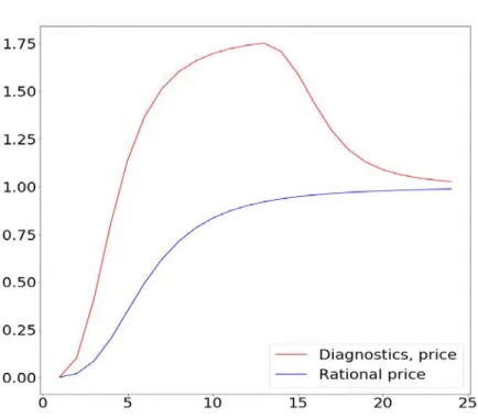
Figure 1 reports the actual price for the average path (no supply shocks) both under diagnostic
expectations (𝜃𝜃= 0.8) and under rational expectations (𝜃𝜃= 0). Under diagnostic expectations, the
equilibrium price exhibits the typical boom bust pattern, where the boom is driven by overreaction to private
signals and prices, while the bust is due to the reversal of expectations at 𝑡𝑡=𝑘𝑘= 12. In the rational model, by contrast, the price monotonically converges to 𝑉𝑉 from below.
12 In BGMS (2018), the estimated signal to noise ratio of the average macroeconomic series was between 3.5 and 4. In the current setting, this should be compared to the precision 𝜎𝜎𝜖𝜖
𝑉𝑉√𝜏𝜏 of the signals received by the traders over some natural
18
Figure 1. Average Price Path
Rational expectations cannot produce over-reaction and price inflation because they constrain assessed
fundamentals to always stay between the prior of zero and the true value 𝑉𝑉. The same is true under
overconfidence, which can generate bubbles only in the presence of short sales constraints (Harrison and Kreps 1978). In our model, a displacement drives continued good news, resulting in a price boom. This leads traders
to focus on the right tail of 𝑉𝑉 and think that the innovation is truly exceptional, causing prices to overreact. The bust occurs at time 𝑡𝑡=𝑘𝑘+ 1, when investors adapt to the displacement, starting to view the innovative asset or technology as the new norm. Here the length 𝑘𝑘 of the boom phase is deterministic, but the
model could be made more realistic by having 𝑘𝑘 stochastic (and even heterogeneous across investors). As in
the analysis of Proposition 1, adaptation to early news causes excess optimism to run out of steam, generating
the bust. Reversal of expectations and prices due to disappointment of prior optimism can help account for the
slowdown of some bubbles, but it is not the only mechanism behind a bust; other factors including bad news
(the housing bubble deflating from 2006 onward), as well as the proximity of a terminal trading date (crucial
in experimental findings), are surely significant. We consider the latter mechanism in Section 4.
Because traders observe independent signals, they have heterogeneous beliefs about the value of the
asset. This creates room for disagreement and trading (Scheinkman and Xiong 2003). Barberis et al. (2018)
19
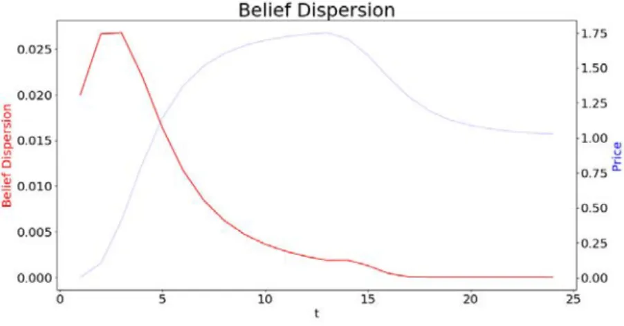
goes by, traders become more confident in their information, which causes them to place stronger weight on
private signals. This effect tends to foster disagreement. At some point, the common price shock becomes so
strong that disagreement declines. We plot the standard deviation of individual beliefs in Figure 2:
disagreement rises in the early part of the boom, but falls as the public signal dominates the private information.
Figure 2. Model-Implied Belief Dispersion
We can also use simulations to describe the dynamics of expectations of future prices. Under mechanical extrapolation, traders project past price increases into the future using the updating rule:
𝔼𝔼𝑖𝑖(𝑝𝑝𝑖𝑖+1) =𝑝𝑝𝑖𝑖+𝛽𝛽(𝑝𝑝𝑖𝑖−1− 𝑝𝑝𝑖𝑖), (13) where 𝛽𝛽 > 0 captures the fixed degree of price extrapolation. In our model, in contrast, traders watch prices in order to infer fundamentals. As a result, price extrapolation arises because high past prices signal high
fundamentals and hence even higher future expected prices.
In Hong and Stein (1999), extrapolation is due to under-reaction, which makes it optimal for
momentum traders to chase the upward trend in prices. In that model, momentum traders form expectations
of future price changes by running simple univariate regressions of current on past price growth. In Glaeser
and Nathanson (2017), investors believe that the price reflects fundamental value. An increase in price is then
interpreted as stronger fundamentals, and leads to extrapolation of high prices into the future. In both models,
as in adaptive expectations, extrapolation is due to the use of simplified (or wrong) models.
This logic suggests a testable difference between mechanical extrapolation models and price learning
20
distorted by 𝜃𝜃. This implies that the degree of extrapolation is not constant over time, but rather depends on the degree of uncertainty concerning fundamentals. In terms of Equation (13), our model predicts that the
updating coefficient 𝛽𝛽 should not be constant, but depends on the extent to which prices are informative. Modest price increases observed in the early stages of a bubble are not very informative about the magnitude
of the fundamental, so the coefficient 𝛽𝛽 should be low. In contrast, a sustained price increase (as observed some time into the bubble) is a solid indicator of a strong fundamental, and should therefore be associated with
a much higher over-reaction, as measured by the coefficient 𝛽𝛽 under diagnostic expectations.
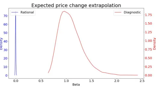
We evaluate these ideas by simulating the model. We run regression (13) using a time series of the
model simulated using the parameters above. We produce 2000 such time series and plot in Figure 3 the
histogram of estimated coefficients for both the diagnostic and the rational model.
Figure 3. Model-Implied Extrapolation Coefficient
The coefficient of price extrapolation implied by the model is positive, between .5 and 1.5. Even
though our investors are entirely forward looking, they appear to mechanically extrapolate past prices. This is
not the case under rational expectations, where the coefficient is negative because traders discount their
information and under-predict the future consensus (and hence price).
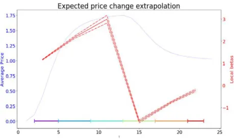
While diagnostic expectations entail a positive extrapolation coefficient on average across the entire
bubble episode (as does mechanical extrapolation), the extrapolation coefficient is the highest when prices are
21
extrapolative coefficient 𝛽𝛽 in each of six buckets, capturing growth, overshooting and collapse of the bubble.13
The results confirm our intuition: price extrapolation is strongest in the making of the bubble when there is rapid learning (the first phase highlighted in blue). This occurs because prices are most informative (relative
to the private signal) in that range, which induces diagnostic traders to update upward more aggressively after
a price rise. At the peak of the bubble, expectations of future prices are significantly above actual prices. After
the bubble bursts, traders adjust their expectations downwards significantly, but not fast enough to converge
to the actual prices. Thus, in this period extrapolation appears negative. Finally, as learning subsides,
extrapolation goes to zero, just as in the rational case.
Figure 4. Time-Dependent Extrapolation
As Figures 3 and 4 show, this model can produce some price convexity and moderate overvaluation.
However, this model precludes large bubbles because for reasonable values of 𝜃𝜃 prices are tethered to the long-term liquidation value. In contrast, prices sometimes strongly overshoot sensible measures of fundamentals.
Second, while learning from prices generates some convexity in the price path, it does not create enough
acceleration to generate increasing growth rate of prices (accelerating returns) seen in the data (Greenwood,
Shleifer, and You 2018). We next show that both features can be attained by adding speculation to our model.
13 To build Figure 3, we simulate 5000 price paths and expected future price paths. We pool simulations and compute the regression 𝔼𝔼𝑖𝑖(𝑝𝑝𝑖𝑖+1) =𝑝𝑝𝑖𝑖+𝛽𝛽(𝑝𝑝𝑖𝑖− 𝑝𝑝𝑖𝑖−1) within buckets of 4 time periods. Figure 3 reports the resulting 𝛽𝛽s and corresponding confidence intervals (running regressions for individual paths and averaging the 𝛽𝛽s yields similar results).
22 4. Speculation
To introduce speculation, we assume that traders have short horizons in the sense that their objective
function at each time 𝑡𝑡 is to resell the asset at time 𝑡𝑡+ 1. The trading game lasts for 𝑇𝑇 rounds, and the traders holding the asset in the terminal date receive its fundamental value. We take 𝑇𝑇 to be exogenously given and deterministic, as in laboratory experiments of bubbles. In real markets, there is no such thing as a terminal
date, but taking a fixed 𝑇𝑇 is a very convenient approximation to a setting in which there is a certain probability that at some point the “speculation game” ends in the sense that most traders attend to fundamentals.
With speculation, diagnostic expectations generate price paths with significantly larger overvaluation
than in the previous models, followed by a price collapse as the terminal date approaches. This occurs because
diagnostic speculators not only overreact to good fundamental news, but also expect to resell to overreacting
buyers in the future, which drives the price today higher. As the terminal date approaches, the prospects for re-trading fade and the bubble bursts. These dynamics are very different from those obtained under rationality.
As in previous Sections, traders hold mean-variance preferences (in particular, expectations are normal
in the diagnostic equilibrium). Away from the terminal date, 𝑡𝑡<𝑇𝑇, trader 𝑖𝑖 chooses demand 𝐷𝐷𝑖𝑖𝑖𝑖 to maximize [𝔼𝔼𝑖𝑖𝑖𝑖(𝑝𝑝𝑖𝑖+1)− 𝑝𝑝𝑖𝑖]𝐷𝐷𝑖𝑖𝑖𝑖−𝛾𝛾2 𝑉𝑉𝑎𝑎𝑓𝑓𝑖𝑖(𝑝𝑝𝑖𝑖+1)𝐷𝐷𝑖𝑖𝑖𝑖2, while his objective at time 𝑇𝑇 is fundamental-based as before. Demand in each period is then given by:
𝐷𝐷𝑖𝑖,𝑖𝑖 =�𝔼𝔼𝑖𝑖,𝑖𝑖 𝜃𝜃(𝑝𝑝 𝑖𝑖+1)− 𝑝𝑝𝑖𝑖� 𝛾𝛾𝑉𝑉𝑎𝑎𝑓𝑓𝑖𝑖(𝑝𝑝𝑖𝑖+1) , 𝑓𝑓𝑓𝑓𝑓𝑓𝑡𝑡= 1, … ,𝑇𝑇 −1, (14) 𝐷𝐷𝑖𝑖,𝑖𝑖 =�𝔼𝔼𝑖𝑖,𝑖𝑖 𝜃𝜃(𝑉𝑉)− 𝑝𝑝 𝑖𝑖� 𝛾𝛾𝑉𝑉𝑎𝑎𝑓𝑓𝑖𝑖(𝑝𝑝𝑖𝑖+1) , 𝑓𝑓𝑓𝑓𝑓𝑓𝑡𝑡=𝑇𝑇. (15) With speculation, demand increases in the expected capital gain 𝔼𝔼𝑖𝑖𝜃𝜃,𝑖𝑖(𝑝𝑝𝑖𝑖+1)− 𝑝𝑝𝑖𝑖 except in the last period 𝑡𝑡=𝑇𝑇, in which traders buy the asset to hold it.
To illustrate the key consequences of speculation, we begin with a model in which there is no learning
from prices. In Section 4.2 we then introduce such learning and compare this formulation to the one in Section
23
which is then used to compute price expectations 𝔼𝔼𝑖𝑖𝜃𝜃,𝑖𝑖(𝑝𝑝𝑖𝑖+1) for next period. In each period, the coefficients of the pricing function are pinned down by equating demand and supply.
In both versions of the speculation model, speculation is itself a source of price reversal as 𝑇𝑇
approaches. We can thus simplify the analysis by assuming that the diagnostic reference is very sluggish, 𝑘𝑘>
𝑇𝑇, so that information about the asset’s value is always assessed compared to the prior 𝑉𝑉= 0.
4.1 Speculation without Learning from Prices
Without learning from prices, we do not need a supply shock, so we assume that the supply of the asset is equal to zero. Aggregating the individual demand functions, prices are pinned down by the conditions:
𝑝𝑝𝑖𝑖=� 𝔼𝔼𝑖𝑖𝜃𝜃,𝑖𝑖(𝑝𝑝𝑖𝑖+1)𝑑𝑑𝑖𝑖, 𝑓𝑓𝑓𝑓𝑓𝑓𝑡𝑡= 1, … ,𝑇𝑇 −1, (16)
𝑝𝑝𝑇𝑇 =� 𝔼𝔼𝑖𝑖𝜃𝜃,𝑇𝑇(𝑉𝑉)𝑑𝑑𝑖𝑖. (17) In the final period 𝑇𝑇, the consensus fundamental value is 𝔼𝔼𝜃𝜃𝑇𝑇(𝑉𝑉) = (1 +𝜃𝜃)𝜋𝜋𝑇𝑇𝑉𝑉, as per Equation (3), leading to the terminal price 𝑝𝑝𝑇𝑇 = (1 +𝜃𝜃)𝜋𝜋𝑇𝑇𝑉𝑉. Under the assumption 𝜃𝜃 ∈ �1
𝑇𝑇 𝜎𝜎𝜖𝜖2
𝜎𝜎𝑣𝑣2,
𝜎𝜎𝜖𝜖2
𝜎𝜎𝑣𝑣2� of Proposition 1, which we maintain, this price is above the fundamental, (1 +𝜃𝜃)𝜋𝜋𝑇𝑇 > 1.14
Consider now the price at 𝑇𝑇 −1. By Equation (16), this price is the consensus expectation as of 𝑇𝑇 −1 of the terminal price 𝑝𝑝𝑇𝑇. To compute this consensus, consider first the expectation held at 𝑇𝑇 −1 by a generic trader 𝑗𝑗. When forecasting the terminal price, this trader must make two assessments. First, he must assess the fundamental value 𝑉𝑉 of the asset. Second, he must assess how future traders will react to noisy signals of the same fundamental value. Because the beliefs of future traders are a random variable, trader 𝑗𝑗 uses the very same diagnostic formula of Equation (2) when representing their distribution. One can interpret this
forecasting process in two ways. First, one can view trader 𝑗𝑗 as placing himself in the shoes of future traders
24
receiving different signals, predicting that these traders will behave the way he would behave in light of the
same signals. Alternatively, one can view trader 𝑗𝑗 as forecasting the behavior of others understanding that they will update diagnostically. In both cases, we continue to rule out the possibility that any trader is
sophisticated enough to be aware of his own diagnosticity, thereby correcting his assessments for it.
Consider how trader 𝑗𝑗 forecasts the beliefs at 𝑇𝑇 of a generic trader 𝑖𝑖 who has observed an average signal ∑𝑇𝑇𝑖𝑖=1𝑠𝑠𝑖𝑖𝑖𝑖
𝑇𝑇 from the initial date to the terminal period. Trader 𝑗𝑗 knows that trader 𝑖𝑖 overreacts to all signals received, forming a terminal estimate 𝔼𝔼𝑖𝑖𝑇𝑇𝜃𝜃(𝑉𝑉) = (1 +𝜃𝜃)𝜋𝜋𝑇𝑇∑𝑇𝑇𝑖𝑖=1𝑠𝑠𝑖𝑖𝑖𝑖
𝑇𝑇 . By averaging across all traders 𝑖𝑖, trader 𝑗𝑗 knows that, if the fundamental value is 𝑉𝑉, the consensus estimate, and hence the equilibrium price at 𝑇𝑇
𝑝𝑝𝑇𝑇 = (1 +𝜃𝜃)𝜋𝜋𝑇𝑇𝑉𝑉.
This prediction is based on the fact that trader 𝑗𝑗 knows that, whichever signals observed by individual traders, they will average out to the true 𝑉𝑉. Of course, trader 𝑗𝑗 does not know the true value of 𝑉𝑉 at 𝑇𝑇 −1; he only has an estimate of it, based on the signals ∑𝑇𝑇−1𝑖𝑖=1𝑠𝑠𝑗𝑗𝑖𝑖
𝑇𝑇−1 observed up to that period. This estimate is diagnostic:
𝔼𝔼𝑗𝑗𝑇𝑇−1𝜃𝜃 (𝑉𝑉) = (1 +𝜃𝜃)𝜋𝜋𝑇𝑇−1∑ 𝑠𝑠𝑗𝑗𝑖𝑖 𝑇𝑇−1 𝑖𝑖=1
𝑇𝑇 −1 .
The diagnostic expectation held at 𝑇𝑇 −1 by trader 𝑗𝑗 about the terminal price is then given by:
𝔼𝔼𝑗𝑗𝑇𝑇−1𝜃𝜃 �𝔼𝔼𝑇𝑇𝜃𝜃(𝑉𝑉)�= (1 +𝜃𝜃)𝜋𝜋𝑇𝑇𝔼𝔼𝑗𝑗𝑇𝑇−1𝜃𝜃 (𝑉𝑉) = (1 +𝜃𝜃)2𝜋𝜋 𝑇𝑇𝜋𝜋𝑇𝑇−1∑ 𝑠𝑠𝑗𝑗𝑖𝑖 𝑇𝑇−1 𝑖𝑖=1 𝑇𝑇 −1 .
This trader uses his signals but he compounds diagnosticity twice. First, he diagnostically overreacts
to his signal, creating an inflated estimate of fundamentals. Second, he expects future traders to over-react to
signals generated by the inflated fundamentals. To see the intuition, imagine that 𝑗𝑗 overestimates the share of future Googles in the population of tech firms to be 7%. He then expects future traders to overreact relative
his assessment and estimate the share of Googles to be, say, 10%. In this way, overreaction to news compounds
25
Because every trader j repeats the same logic, by averaging across all of them, the consensus forecast
held at time 𝑇𝑇 −1 about the terminal price, and thus the equilibrium price at 𝑇𝑇 −1 is given by:
𝑝𝑝𝑇𝑇−1= (1 +𝜃𝜃)2𝜋𝜋𝑇𝑇𝜋𝜋𝑇𝑇−1𝑉𝑉. (18) To gauge the role of diagnostic expectations, suppose that traders are rational, so 𝜃𝜃= 0. In this case, the price at 𝑇𝑇 −1 is lower than the terminal price, because 𝜋𝜋𝑇𝑇−1< 1. As a result, under rationality speculation causes the price to rise as the terminal date is approached. It is well known that speculation under rationality
leads to initial under-reaction, and thus to a rising price path (Allen et al. 2006). The intuition is that rational
traders discount their signals and expect future traders to do the same. As a result, they do not expect to be able
to resell the asset for a very high price, which keeps the current price low.
With diagnosticity, even a modicum of overreaction dramatically changes the calculus. When 𝜃𝜃 > 0, it is entirely possible that the price drops at the terminal date. This is true if and only if:
𝑝𝑝𝑇𝑇−1>𝑝𝑝𝑇𝑇 ⟺(1 +𝜃𝜃)𝜋𝜋𝑇𝑇−1 > 1.
If traders overestimate the fundamental value at time 𝑇𝑇 −1, i.e. (1 +𝜃𝜃)𝜋𝜋𝑇𝑇−1> 1, then the price at 𝑇𝑇 −1 is above both fundamentals and the terminal price. Indeed, by overestimating 𝑉𝑉, traders believe that future traders will overreact to this estimate, compounding overreaction twice. But then, the expectation to sell to
these bullish traders in the future raises the current price of the asset.
In sharp contrast with the rational case, which leads to a monotone rising price path, diagnostic
expectations introduce the opposite effect. By creating overreaction, they imply that prices decline toward the
terminal date, reflecting an initial strong overvaluation of the asset.
To study the implications of 𝜃𝜃> 0 fully, we need to iterate the same logic backward to earlier periods until the initial date 𝑡𝑡= 1. It is immediate to see that the full path of equilibrium prices obtained by iterating Equation (18) backwards is described by:
𝑝𝑝𝑖𝑖 = (1 +𝜃𝜃)𝑇𝑇−𝑖𝑖+1�� 𝜋𝜋𝑖𝑖 𝑇𝑇
𝑖𝑖=𝑖𝑖 � 𝑉𝑉, (19) which implies the following result.
26
Proposition 4 Define the geometric average of all signal to noise ratios 𝜋𝜋� ≡[∏𝑇𝑇𝑖𝑖=1𝜋𝜋𝑖𝑖]1𝑇𝑇. Then, if 𝜃𝜃 ∈
�1𝑇𝑇𝜎𝜎𝜖𝜖2
𝜎𝜎𝑣𝑣2,1−𝜋𝜋�𝜋𝜋� �, where1−𝜋𝜋�𝜋𝜋� <𝜎𝜎𝜖𝜖 2
𝜎𝜎𝑣𝑣2, the speculative price dynamics exhibit the three bubble phases. In particular:
1. The price starts below fundamental, 𝑝𝑝1<𝑉𝑉, and gradually increases above fundamentals, reaching its maximum at the smallest time 𝑡𝑡̂ for which (1 +𝜃𝜃)𝜋𝜋𝑖𝑖̂ > 1.
2. From 𝑡𝑡=𝑡𝑡̂ onwards the price monotonically declines toward 𝑝𝑝𝑇𝑇.
With diagnostic expectations, speculative dynamics can generate both the sluggish upward price
adjustment typical of underreaction (provided 𝜃𝜃 is not too large), the price inflation relative to fundamentals typical of overreaction (provided 𝜃𝜃 is not too small), and the bust phase in which prices collapse, which here is driven by the reduction in the available rounds of reselling.
Because (1 +𝜃𝜃)𝜋𝜋�𝑇𝑇 < 1, individual traders underreact to the aggregate information in the first period. The logic is the same as before: individual uncertainty about 𝑉𝑉 is still very large. Traders are not only cautious in estimating 𝑉𝑉, but also think that next period buyers will be cautious as well. This effect curtails the expected resale price and demand for the asset today, keeping its price low. As time goes by, traders acquire more
information, become more confident, and start using it more aggressively. They become more optimistic about
the signals future buyers will get, more confident about future buyers’ over-optimism, and the price starts
increasing. As traders gain confidence, the possibility of multiple rounds of reselling to over-reacting traders
dramatically boosts price, which overshoots 𝑉𝑉. The price then starts declining as the terminal date 𝑇𝑇
approaches, because there are fewer and fewer rounds of trading and thus less scope for reselling to
overreacting buyers.
Once again, under rationality, the dynamics of speculation do not yield a hump shaped price path.
Given 𝜃𝜃= 0, traders rationally anticipate that future traders will have lower signals than they do, and that they will in turn discount those signals, resulting in depressed prices. Because traders receive information over
time, price grows monotonically and approaches 𝑉𝑉 from below. It displays momentum but not overshooting