TARP’S EFFECT ON BANKS'
REPORTED PERFORMANCE
An empirical study on TARP
contributions’
relative sizes’ effect on bank performance
Master’s Thesis
Sakari Saarela
Fall 2016
Accounting
Approved in the Department of Accounting __ / __20___ and awarded the grade
Aalto University, P.O. BOX 11000, 00076 AALTO www.aalto.fi Abstract of master’s thesis
i
Author Sakari Saarela
Title of thesis TARP’s Effect on Banks' Reported Performance
Degree Master’s Degree
Degree programme Accounting
Thesis advisor(s) Henry Jarva
Year of approval 2016 Number of pages 62 Language English
Abstract
The financial crisis that began in August 2007 has been the most significant challenge to the banking industry and financial system as a whole in the U.S. since the great recession in the 1930s. It is one of the most studied series of events in the modern economic research. Government intervention is a controversial measure taken to mitigate the widespread negative effects resultant form a banking crisis.
This thesis studies the U.S. Treasury’s Troubled Asset Relief Program’s (“TARP”) effect on the banks’ performance by the means of a review of earlier literature on the subject and by conducting an empirical study. The empirical study uses accounting-based profitability and balance sheet based indicators in determining the performance of the banks. Three regression models are estimated in the empirical study. The models are formulated to answer the research question “Were the TARP funds allocated optimally and fairly among the U.S. banking industry’s entities?” by studying the TARP funds’ size’s – relative to the recipients’ total assets – effect on the banks’ performance one year after the TARP capital injections.
Earlier literature has found that TARP e.g. worsened the operating efficiency of the banks participating in it, but allowed competitive advantages, and an increase in market share and market power for its recipients. Earlier literature has also concluded that TARP induced moral hazard among banks.
The results of the empirical study conducted in this thesis suggest that the relative size of received TARP funds has had an effect on the banks’ performance one year after the TARP injections. The relative size of received TARP funds has had a clear positive effect on return on loans. However, the effect on other performance indicators is mixed. The profitability indicators subject to the most managerial discretion in terms of result management have been affected negatively by the relative size of received TARP funds, which could indicate that the receipt of a large TARP injection has encouraged managers to unravel already accumulated writedown backlogs. The results of the empirical study also find that banks’ prior performance has had an effect on the banks’ probability to receive TARP funds: more poorly performing banks were more likely to receive TARP funds.
The possibility of the TARP funds affecting the bank managers’ usage of discretionary items opens an interesting possibility for accounting research to further study the phenomenon. The results of this study call for research on the usage of discretionary items before, during, and after TARP in U.S. banks, and the relative TARP funds’ size’s effect on these.
Aalto-yliopisto, PL 11000, 00076 AALTO www.aalto.fi Maisterintutkinnon tutkielman tiivistelmä
ii
Tekijä Sakari Saarela
Työn nimi TARP-ohjelman vaikutus pankkien raportoituun suorituskykyyn
Tutkinto Kauppatieteiden maisterin tutkinto
Koulutusohjelma Accounting
Työn ohjaaja(t) Henry Jarva
Hyväksymisvuosi 2016 Sivumäärä 62 Kieli Englanti
Tiivistelmä
Vuoden 2007 elokuussa alkanut finanssikriisi on ollut merkittävin haaste yhdysvaltalaiselle pankkialalle ja koko rahoitusjärjestelmälle 1930-luvun Suuren laman jälkeisessä historiassa. Finanssikriisi on yksi modernin taloustieteen tutkituimmista tapahtumasarjoista. Valtion rahoittamat apuohjelmat ovat kiistanalainen keino, jolla pyritään lieventämään pankkikriisien merkittäviä negatiivisia vaikutuksia kokonaistalouteen.
Tämä tutkielma tutkii Yhdysvaltain valtionvarainministeriön (U.S. Treasury) Troubled Asset Relief Program (“TARP”) -rahoitusapuohjelman vaikutusta pankkien suorituskykyyn tutkimalla aikaisempaa kirjallisuutta, sekä empiirisellä tutkimuksella. TARP-ohjelman vaikutusta pankkeihin tutkitaan raportoituihin talouslukuihin perustuvilla, kannattavuutta ja taseen koostumusta mittaavilla indikaattoreilla mitattuna.
Tutkielman empiirisessä osiossa käytetyt regressiomallit on luotu vastaamaan
tutkimuskysymykseen ”Allokoitiinko TARP-ohjelman yhteydessä sijoitetut optimaalisesti ja reilusti yhdysvaltalaisten pankkialan toimijoiden kesken?” tutkimalla TARP-ohjelman yhteydessä sijoitettujen varojen vastaanottajan kokoon suhteutetun määrän vaikutusta pankkien suorituskykyyn vuosi TARP-sijoitusten jälkeen.
Aikaisemmat tutkimukset ovat muun muassa todenneet, että TARP-ohjelma heikensi pankkien operatiivista tehokkuutta, mutta samanaikaisesti nosti TARP-sijoituksia vastaanottaneiden pankkien markkinaosuuksia sekä markkinavoimaa ja antoi näille kilpailuetua. Aikaisempien tutkimusten mukaan TARP-ohjelma myös loi moraalikatoa pankkien keskuudessa.
Tämän tutkielman empiirisen tutkimuksen tulokset näyttävät TARP-ohjelman yhteydessä sijoitettujen pääomien suhteellisen koon vaikuttaneen vastaanottavien pankkien suorituskykyyn vuosi TARP-sijoitusten jälkeen. TARP-sijoituksen suhteellisella koolla on ollut selvä positiivinen vaikutus lainojen tuottavuusasteeseen. TARP-sijoituksen suhteellisen koon vaikutus muiden kannattavuusindikaattoreiden kehitykseen on ollut vaihteleva. Eniten johdon tulosohjaukselle alttiit kannattavuusindikaattorit ovat reagoineet negatiivisimmin TARP-sijoitusten suhteelliseen kokoon, joka voi tarkoittaa sitä, että suuren TARP-sijoituksen vastaanottaminen on saanut vastaanottajapankkien johtajat purkamaan huonon taloudellisen jakson aikana kertynyttä alaskirjaustarvetta. Tämän tutkielman tulokset osoittavat myös, että pankkien TARP-ohjelmaa edeltävä suorituskyky on vaikuttanut todennäköisyyteen vastaanottaa TARP-sijoituksia: heikompikuntoiset pankit saivat todennäköisemmin TARP-sijoituksia.
Mahdollinen TARP-sijoituksen vaikutus vastaanottajapankkien johtajien harkinnanvaraisten erien käyttöön avaa mielenkiintoisen mahdollisuuden laskentatoimen tutkimukselle kyseisen ilmiön edelleen tutkimiseen. Tämän tutkielman tulokset johdattelevat tulevaa tutkimusta selvittämään harkinnanvaraisten erien käyttöä ennen TARP-ohjelmaa, sen aikana ja sen jälkeen, sekä TARP-sijoitusten suhteellisten kokojen vaikutusta harkinnanvaraisten erien käyttöön.
iii TABLE OF CONTENTS
1. INTRODUCTION ... 1
1.1. BACKGROUND AND MOTIVATION ... 1
1.2. RESEARCH QUESTION AND CONTRIBUTION... 5
1.3. STRUCTURE ... 6
2. MEASURING BANK PERFORMANCE ... 8
2.1. BANK PERFORMANCE IN GENERAL ... 8
2.2. BANK PROFITABILITY INDICATORS ... 8
2.3. BANK BALANCE SHEET INDICATORS ... 9
2.4. BANK EFFICIENCY ... 10
2.5. BANK PERFORMANCE FROM REGULATORS’ VIEWPOINT ... 10
3. GOVERNMENT INTERVENTION IN THE BANKING INDUSTRY ... 12
3.1. GOVERNMENT INTERVENTION’S EFFECT ON BANK PERFORMANCE ... 12
3.1.1. Government Intervention’s Effect in General ... 13
3.1.2. Comparisons of Means of Government Intervention ... 14
3.2. TARP’S EFFECT ON BANK PERFORMANCE ... 15
4. RESEARCH DESIGN ... 20
4.1. HYPOTHESES... 20
4.2. DATA ... 21
4.2.1. TARP Transaction Data ... 21
4.2.2. Bank Financials – Base Data ... 23
4.2.3. Bank Financials – Performance Effect Model’s Sample ... 24
4.2.4. Bank Financials – Lagged Performance Effect Model’s Sample ... 24
4.2.5. Bank Financials – TARP Receipt Probability Model’s Sample ... 24
iv
4.3.1. Received TARP Funds’ Relative Size (Independent Variable) ... 25
4.3.2. TARP Receipt Dummy Variable (Independent Variable) ... 25
4.3.3. Bank Performance Indicators (Dependent Variables) ... 26
4.3.4. Control Variables... 28
4.4. REGRESSION MODELS ... 29
4.4.1. Core Model – Performance Effect Model ... 29
4.4.2. Lagged Performance Effect Model ... 30
4.4.3. TARP Receipt Probability Model ... 31
5. RESULTS ... 32
5.1. SUMMARY STATISTICS ... 32
5.2. STUDY OF CORRELATIONS ... 37
5.2.1. Correlations in the Base Data ... 37
5.2.2. Correlations in the Performance Effect Model’s Sample ... 39
5.3. RESULTS OF THE PERFORMANCE EFFECT MODEL ... 41
5.3.1. Profitability Effect Results ... 42
5.3.2. Balance Sheet Effect Results ... 44
5.4. RESULTS OF THE LAGGED PERFORMANCE EFFECT MODEL ... 45
5.4.1. Profitability Effect Results ... 47
5.4.2. Balance Sheet Effect Results ... 48
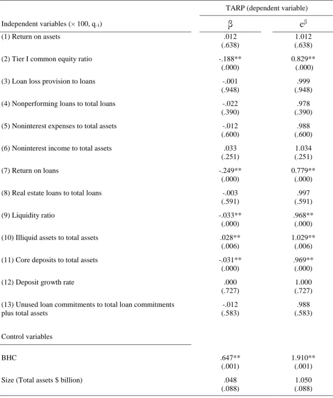
5.5. RESULTS OF THE TARP RECEIPT PROBABILITY MODEL ... 48
6. CONCLUSIONS... 52
6.1. CONCLUSIONS ON TARP’S OPTIMAL AND FAIR ALLOCATION ... 52
6.2. CONCLUSIONS ON TARP’S EFFECT ON PERFORMANCE ... 52
6.3. TOPICS FOR FURTHER RESEARCH ... 54
v TABLE OF FIGURES
Figure 1. Capital Injections and Repayments under TARP ... 3
Figure 2. Base Data's High-Variance Variables ... 34
LIST OF TABLES Table 1. Timeline of Events Related to TARP Capital Infusions (Bayazitova & Shivdasani 2012) ... 4
Table 2. Definition of Bank Performance Indicators ... 28
Table 3. Summary Statistics for the Base Data ... 33
Table 4. Summary Statistics for the Performance Effect Model's Sample ... 35
Table 5. Selected Summary Statistics by TARP Status ... 36
Table 6. Correlations in the Base Data ... 38
Table 7. Correlations in the Performance Effect Model’s Sample ... 40
Table 8. Results of the Performance Effect Model ... 41
Table 9. Results of the Lagged Performance Effect Model ... 47
Table 10. Results of the TARP Receipt Probability Model ... 50
APPENDICES Appendix 1. Descriptions of Call Report Codes Used ………...61
1
1.
INTRODUCTION
This section provides the background for the studied phenomenon and sets out the motivation for studying the Troubled Asset Relief Program’s and specifically Capital Purchase Program’s and Targeted Investment Program’s effect on banks’ performance. This section also lays out the research questions for the literature review and empirical study of this thesis, and briefly discusses this thesis’ contribution to the research of the subject. The structure of this thesis is described in chapter 1.3 of this section.
1.1.BACKGROUND AND MOTIVATION
The financial crisis that began in August 2007 has been the most significant challenge to the banking industry and financial system as a whole in the U.S. since the great recession in the 1930s (Calomiris & Khan 2015; Hoshi & Kashyap 2010). It is one of the most studied series of events in the modern economic research. In October 3rd, 2008, the United States Congress accepted a proposal by the U.S. Department of the Treasury (the “Treasury”) regarding a program under which the U.S. government invested over $204 billion into 707 troubled banking industry companies during 2008 and 2009 (Hoshi & Kashyap 2010; U.S. Department of the Treasury 2016a). This program is the Capital Purchase Program (“CPP”), which was created under the Troubled Asset Relief Program (“TARP”), which, in turn, was created as part of the Emergency Economic Stabilization Act (U.S. Department of the Treasury 2010). The investments made under the CPP continued from the first investment into eight very large banks on 28th of October, 2008 until 29th of December, 2009 (U.S. Department of the Treasury 2016a). The TARP was initially approved to invest a total of $700 billion into distressed assets of which the CPP’s share was $250 billion (Veronesi & Zingales 2010; U.S. Department of the Treasury 2010).
CPP funds were applied for by submitting a two-page form to each financial institution’s primary banking regulator: The Federal Deposit Insurance Corporation, the Federal Reserve, the Office of the Comptroller of the Currency, or the Office of Thrift Supervision. The applications were reviewed using the “Camels” rating system, which evaluates six indicators: Capital adequacy, Asset quality, Management, Earnings, Liquidity, and Sensitivity to market risk. The successful applicants issued preferred stock for the Treasury. The preferred stock had to pay quarterly dividends yielding 5 % annually for the first five years and 9 % thereafter. The
2
amount invested was at the discretion of the Treasury, but always 1–3 % of the investee’s risk-weighted assets or $25 billion at maximum. If the investee was a public company, the Treasury required ten-year warrants for the company’s common stock. (Duchin & Sosyura 2014.)
On October 28th, 2008, just over a month after the bankruptcy of Lehman Brothers, the first investments under the CPP were made by the Treasury. Out of the $250 billion initially allocated for CPP, some $205 billion were ultimately invested in 707 financial institutions. (U.S. Department of the Treasury 2016b.) In addition to CPP, the Treasury created a complementary program, the Targeted Investment Program (“TIP”), which comprised two investments of $20 billion each to Citigroup Inc. and Bank of America in December 2008 and January 2009, respectively (Calomiris & Khan 2015). The TIP investments brought the total amount invested under the programs to approximately $245 billion.
The recipients of largest amounts of CPP and TIP investments combined were Citigroup Inc. ($45 billion), Bank of America ($45 billion), JPMorgan Chase & Co., and Wells Fargo & Co., with $25 billion each. In total, nine financial institutions received more than $5 billion per company and 27 more than $1 billion, respectively (U.S. Department of the Treasury 2016b; Calomiris & Khan 2015.) On 27.1.2016, the banks that had received TARP funds had repaid approximately $266 billion to the Treasury, while approximately $258 million of the original investments was outstanding (U.S. Department of the Treasury, 2016b). The investments and repayments under TARP are shown in Figure 1 below.
3
FIGURE 1. CAPITAL INJECTIONS AND REPAYMENTS UNDER TARP
The figure below presents the capital injections made by the Treasury under TARP and the repayments made by the funded banks on a timeline between 28.10.2008 and 27.1.2016. The figures include combined data for CPP and TIP (U.S. Department of the Treasury 2016b). The total investment under TARP (only CPP and TIP) by the Treasury was approximately $245 billion. The banks that had received TARP funds have repaid approximately $266 billion to the Treasury.
___________________________________________________________________________
___________________________________________________________________________
TARP was directed towards financial institutions including bank holding companies (“BHC”), commercial banks, savings and loan institutions and other thrifts, and under 8 % of the TARP fund recipients were savings and loan institutions or other thrifts (Berger & Roman 2015). A timeline of the events around the TARP programs is presented in Table 1 below. This thesis studies the effect on CPP and TIP (hereafter together referred to as “TARP”) on BHCs and commercial banks, which are together referred to as banks. The exclusion of savings and loan institutions and other thrifts is due to their financial information not being fully compatible with banks and due to the fact that they compete in different ways than banks (Berger & Roman 2015). These exclusions are in line with earlier studies conducted by e.g. Harris et al. (2013), Cornett et al. (2013), and Berger & Roman (2015).
4
TABLE 1. TIMELINE OF EVENTS RELATED TO TARP CAPITAL INFUSIONS (BAYAZITOVA & SHIVDASANI 2012)
The table below presents a timeline of the events around the TARP capital injections in 2008–2009.
October 3, 2008: President Bush signs into law the Emergency Economic Stabilization Act of 2008, which establishes the $700 billion Troubled Asset Relief Program (TARP).
October 13, 2008: U.S. Treasury interim assistant secretary Neel Kashkari announces a standardized program to purchase equity in a broad array of financial institutions.
October 14, 2008: The U.S. Treasury announces the Capital Purchase Program (CPP), which allows U.S. financial institutions to apply for a preferred stock investment by the U.S. Treasury. Nine large financial organizations announce they will subscribe to the facility in an aggregate amount of $125 billion. The FDIC creates a new Temporary Liquidity Guarantee Program to guarantee the senior debt of all FDIC-insured institutions as well as deposits through June 30, 2009.
November 14, 2008: The deadline for publicly held financial institutions to apply for a CPP preferred stock investment by the U.S. Treasury.
February 4, 2009: The U.S. Treasury modifies restrictions on executive compensation for TARP participants. The total annual compensation for senior executive officers is limited to $500,000, except for long-term restricted stock awards. Golden parachutes are prohibited for the top ten senior executives, and the next twenty-five executives are prohibited from receiving golden parachute payments greater than one year’s compensation upon severance. Bonus claw-back provisions were extended from the top five executives to the next twenty- five executives.
February 10, 2009: U.S. Treasury Secretary Timothy Geithner announces the Financial Stability Plan involving forward-looking loss assessments for nineteen U.S. banks with assets exceeding $100 billion, the Capital Assessment Program (CAP) whereby the U.S. Treasury will purchase preferred stock convertible to common equity in eligible banks, the creation of a Public-Private Investment Fund to acquire troubled loans and assets from financial institutions, expansion of the Federal Reserve’s Term Asset-Backed Securities Loan Facility (TALF), and new initiatives to stem residential mortgage foreclosures and to support small business lending.
February 17, 2009: President Obama signs into law the American Recovery and Reinvestment Act of 2009, which includes a variety of spending measures and tax cuts intended to promote economic recovery. The act includes most of the executive compensation restrictions for TARP participants announced on February 4, 2009. The act includes additional compensation restrictions for TARP participants with a prohibition on bonuses, retention awards, or incentive compensation exclusive of long-term restricted stock awards that do not exceed one-third of the annual compensation.
February 23, 2009: The U.S. Treasury and federal bank regulatory agencies issue a joint statement in which they reiterate that under CAP, capital will be provided in the form of mandatorily convertible preferred stocks, and previous capital injections under CPP will also be eligible to be exchanged for these shares.
February 24, 2009: Federal Reserve chairman Ben Bernanke clarifies to Congress that the bank stress tests are not a precursor to nationalization of banks.
February 25, 2009: The U.S. Treasury publishes a white paper, term sheet, and FAQs containing details on the CAP program.
February 26, 2009: Iberiabank Corp. files notice with the Treasury Department that it will redeem all 90,000 outstanding shares of U.S. Treasury preferred stock for a redemption price of $90.6 million.
March 19, 2009: The U.S. Congress proposes and passes H.R. 1586 in under twenty-four hours with an overwhelming margin. The bill imposes a punitive excise tax of 90% on all employee bonus payments made, retroactive to January 1, 2009, by institutions that have received $5 billion or more in TARP capital.
March 31, 2009: Four bank holding companies (Marin Bancorp., Iberiabank Corp., Old National Bancorp., and Signature Bank) announce that they have redeemed all of the preferred shares issued to the U.S. Treasury under CPP.
April 24, 2009: The Federal Reserve Board publishes a white paper describing the process and methodology employed by federal banking supervisory authorities in their forward-looking assessment (stress test) of large U.S. bank holding companies.
5 TABLE 1. CONTINUED
May 6, 2009: The Wall Street Journal reports that results of the government’s stress tests for several banks have been leaked to the media. It reports that American Express, Bank of New York Mellon, Capital One Financial, Goldman Sachs, MetLife, and JPMorgan Chase will not need to raise additional capital, while Bank of America needs $34 billion, Wells Fargo requires $15 billion, and GMAC needs $11.5 billion. The Journal reports that Citigroup, State Street, Morgan Stanley, and Regions Financial will also need additional capital.
May 7, 2009: The Federal Reserve releases the results of the Supervisory Capital Assessment Program (SCAP) for the nineteen largest U.S. bank holding companies. The assessment finds that ten firms need to add $185 billion to capital but that transactions and revenues since the end of 2008 have reduced the capital shortfall to $75 billion. Banks that need to augment capital will be required to develop a detailed plan to be approved by its primary supervisor within thirty days and to raise the additional capital by November 2009.
June 10, 2009: The U.S. Treasury Department issues detailed rules regarding the limitations on executive and employee compensation imposed under the American Recovery and Reinvestment Act of 2009 for companies receiving funds under TARP. Treasury secretary Timothy Geithner also issues a press release on compensation principles.
December 31, 2009: The authority of the U.S. Treasury to purchase capital in financial institutions under CPP terminates, as specified in the Emergency Economic Stabilization Act of 2008.
Implementing such an enormous-scale government-funded program is always a major decision affecting the global economic history. The use of taxpayer money on the revitalization of the financial sector is a sensitive topic as it is highly costly to taxpayers (Granja 2013), and it has been proven to cause a moral hazard as the banks receiving a “too-big-to-fail” status are incentivized to allocate their capital towards more risky uses (O’Hara & Shaw 1990; Hoque 2013; Harris et al. 2013). Due to the aforementioned factors, the optimal and fair allocation of such government funds is highly important.
1.2.RESEARCH QUESTION AND CONTRIBUTION
Unintended effects of government guarantees on different entities’ incentives have been systematically studied since the 1970s by e.g. Ehrenberg & Oaxaca (1976) and Mortensen (1977), who studied the subject of unemployment insurances’ effect on employees’ employment decisions (Duchin & Sosyura 2014). Prior research (e.g. Ding et al. 2013) has covered the topic of government intervention’s effect on banks’ reported performance in geographies other than the United States. Government intervention’s, including the CPP’s, effect on banks’ stock performance and financial results has been studied in the U.S. as well (e.g. Berger & Roman 2015; Farruggio et al. 2013; Harris et al. 2013; Liu et al. 2013). The previous research has, however, only studied the phenomenon by labeling the banks that received any CPP/TARP funds as “TARP banks” and others as “non-TARP banks”. This thesis’s approach complements the prior research by widening the research basis comprising
6
logistic regression studies by taking into account the relative size of the TARP contribution per bank.
The research question of this thesis is:
Were the TARP funds allocated optimally and fairly among the U.S. banking industry’s entities?
The research question is answered through a literature review studying government intervention’s and TARP’s effect on bank performance, and by conducting an empirical study analyzing the effects of relative TARP injections’ sizes on the banks’ performance. If the TARP funds have been allocated optimally and fairly, there should not be an observable effect on the banks’ performance compared to one another resultant from the relative size of received TARP funds. If the banks receiving larger amounts of TARP funds in relation to their total assets have systematically outperformed other banks one year after the capital injections, the funds have been unjustly allocated. This is due to the fact that the TARP funds’ target was to remedy troubled financial institutions, and if these troubled institutions have been systematically brought to a superior performance level through subsidy-like government capital, the funds have not been allocated optimally from the overall economy’s viewpoint. This type of government capital injections would potentially further invoke hazardous behavior from the banks as the banks that had assumed the most risk in the past would be rewarded for realized risk in this scenario. The research question, being of highly fundamental nature, cannot be answered through this thesis alone. This thesis seeks to contribute to the already vast literature answering the research question and to provide a basis and guidance for further research contributing to answering the research question.
1.3.STRUCTURE
This thesis uses two main methods to study the effect the relative size of received TARP funds has had on the U.S. banks’ performance: a literature review to provide adequate background, and an empirical study. The literature review is conducted in the second and third chapters of this thesis. The first literature review section discusses bank performance measurement methods. The third chapter begins with a section studying government intervention’s effect on bank performance in general, globally. Thereafter, TARP’s effect on performance is studied through literature review.
7
The fourth chapter of this thesis presents the research design of the empirical study. The fourth chapter includes sections describing the hypotheses, data used, variables formed, and the three regression models formulated based on the data and variables. The fifth chapter then presents the results of the regression models including separate sections for descriptive statistics, studies of correlations, and for each of the models’ results. The sixth and last chapter of this thesis draws the conclusions from the literature review and empirical study conducted, and suggests topics for further research on the subject of TARP’s effect on bank performance.
8
2.
MEASURING BANK PERFORMANCE
Banks report their profit and loss statements and balance sheets in a different manner to normal companies, due to which the performance measurements of banks are different than those of normal companies. In order to provide basis for this thesis’ subject of analyzing TARP’s effect on bank performance, this section provides a brief review of bank performance measurement. Bank profitability and balance sheet measures are addressed, after which a brief introduction of bank efficiency is provided.
2.1.BANK PERFORMANCE IN GENERAL
The primary objective of any financial system is to provide information for investors regarding the reporting entities for the use of investors, and in this sense the financial reporting of banks is no different to other entities (Bushman 2014). However, banks are in many respects different to companies competing in other industries and have a set of characteristics that are unique to the financial sector (Bushman 2014). Due to this, banks’ financial reports differ materially from those of non-financial entities. Even though performance measurement usually varies between all different industries, banks’ performance measurement has an unusually high amount of dissimilarities with other industries due to the industry-specific financial reporting.
Bank performance is often measured by market information, i.e. stock prices (see e.g. (Fahlenbrach et al. 2012) due to the stock prices theoretically fully reflecting all publicly available information as they unbiasedly react to information in real time (Ball, Ray; Brown 1968). Therefore, stock prices do not only contain information on the banks fundamentals, but also on expected government actions (Bond & Goldstein 2015). However, attempting to contribute to the accounting literature in bank performance research, this thesis focuses on bank performance measured by accounting-based information in order to measure the actual realized financial performance of the banks after the receipt of TARP funds.
2.2.BANK PROFITABILITY INDICATORS
A bank’s income statement differs from a regular company’s income statement. It is typically divided into four components: net interest income, provision for loan losses, net non-interest income, and securities gains and losses (Beatty & Liao 2014). The regulation concerning result
9
planning is stricter for banks than for ordinary companies and therefore e.g. return on assets (net income after taxes as a percent of total assets) and return on loans (interest and fees on loans as a percent of total loans and leases) are the most fundamental accounting-based measures of profitability for banks. Return on assets is used as the main accounting-based measure of bank profitability by e.g. Blackwell et al. (1994), Hryckiewicz (2014), Lin & Zhang (2009), and Ding et al. (2013). Return on loans is used as one of the core indicators of bank profitability by e.g. Cornett et al. (2013) and Logue & Rivoli (1992).
2.3.BANK BALANCE SHEET INDICATORS
In addition to measuring profitability, accounting-based information can be used to measure e.g. liquidity, solvency, and other balance sheet based performance indicators. Banks’ balance sheets are also reported on a format different than ordinary companies’ balance sheets. The most used balance sheet based bank performance measures include tier I common equity ratio (used by e.g. Harris et al. 2013, Cornett et al. 2013, Li 2013, and Fahlenbrach et al. 2012) which is an indicator specific to banks and measures the amount of tier I common equity as regulated by Basel Committee on Banking Supervision (2011) in relation to the banks total assets. Liquidity ratio (used by e.g. Granja 2013, Cornett et al. 2013, and Hryckiewicz 2014) is a highly used bank balance sheet indicator, which measures the cash and investment securities as a percentage of total assets. Different nonperforming loan ratios (used by e.g. Lin & Zhang 2009, Nakashima 2016, and Farruggio et al. 2013) are frequently used measures, which include a component formed by summing loans and leases that are 90 or more days due, nonaccruing loans and leases, and other real estate owned, which is then divided by e.g. total loans and leases. Another frequently used balance sheet based bank performance indicator is core deposits to total assets (used by e.g. Beatty & Liao 2014, Cornett et al. 2013, and James 1991), which measures the sum of transactions deposits and non-transaction deposits of under $100 000 as a percentage of total assets.
In addition to the aforementioned balance sheet indicators, bank balance sheet information is used as a measure of the banks’ risk-taking (Black & Hazelwood 2013). Riskiness of an asset is also one of the factors influencing the asset’s performance, as a higher performance is required of a more risky asset (Sharpe 1966) and thus a lower risk enhances the risk-adjusted performance of an asset, here a bank. Bank risk can be measured by the aforementioned balance sheet based indicators. In addition, e.g. expected delayed loan loss provisions, which is derived
10
from bank balance sheet information, can be used to measure bank risk (Bushman & Williams 2015).
2.4.BANK EFFICIENCY
In addition to profitability and balance sheet structure indicators, the banking industry is evaluated on the basis of its actors’ efficiency. This thesis does not concentrate on bank efficiency, but the topic is briefly discussed in order to provide a more comprehensive context for bank performance measurement. Efficiency as it is meant in the banking literature is an indicator specific to the banking industry. Bank efficiency is measured as the relative efficiency score’s distance from the efficient frontier first introduced by Markowitz (1952) (Bonin et al. 2005).
Assessing the efficiency of banks has been a core topic of the research relating to bank performance for decades. The main factor causing controversy in the research field is the appropriate inputs and outputs of the banks’ production process. Even though wide consensus regarding the measurement of bank efficiency does not exist, it is most commonly accepted that the main inputs are fixed assets and employees. (Holod & Lewis 2011.)
2.5.BANK PERFORMANCE FROM REGULATORS’ VIEWPOINT
The fact that the recent financial crisis resulted in a need for government bailouts of banks brought more into discussions the concerns regarding proper monitoring of banks’ risk taking incentives, which led to demands for additional equity capital to be held by banks. In fact, one of the most central of the items regulated in Basel III is tier I common equity. (Beatty & Liao 2014.) This is one of the key indicators of riskiness of a bank’s assets, which is arguably the most pressing fundament the regulators are concerned with. For example Barth & Landsman (2010), Nakashima (2016), and Akins et al. (2016) use riskiness of bank assets as one of the key performance indicators.
The capital requirements are also in the core of the most central regulatory bank performance indicator regarding the U.S. banks in the wake of TARP, i.e. the CAMELS rating system. This system was used to evaluate the TARP applicants. CAMELS stands for Capital adequacy, Asset quality, Management, Earnings, Liquidity, and Sensitivity to market risk. For example Duchin
11
& Sosyura (2014) assess bank performance through estimating CAMELS proxies for their sample. They use tier I common equity ratio as Capital adequacy, the negative of noncurrent loans and leases as a percentage of total loans and leases as Asset quality, negative of the number of corrective actions taken against executives by regulators as Management quality, ROE as Earnings, cash divided by deposits as Liquidity, and ratio of absolute difference between short-term assets and short-term liabilities to earning assets as Sensitivity to market risk. Fairly dissimilar proxies have also been used, as e.g. Beatty & Liao (2011) and Bushman & Williams (2015) use ROA as a proxy for Management.
One measure for bank performance from the overall economy’s viewpoint is their ability to borrow and lend. For example Calomiris & Khan (2015) and Li (2013) use different measures of lending activity as bank performance indicators in their studies. Calomiris & Khan (2015) use the supply of lending as a performance indicator in their study of TARP banks. Likewise, Li (2013) uses the credit supply measured by all types of loans and the level of new loans issued as bank performance indicators in his study.
12
3.
GOVERNMENT INTERVENTION IN THE BANKING INDUSTRY
This section compiles the earlier literature on the subject of government intervention’s and TARP’s effect on banks’ performance. This section does not purport to include a review of all relevant studies published on the subject, but seeks to review the most relevant parts of the studies concentrated on the phenomenon in question. First, this section reviews earlier literature on different types of government interventions’ effect on bank performance in general, and second, studies on TARP’s effect on bank performance are reviewed.
This thesis focuses only on the government intervention conducted in the form of government-led programs that have subsidy-like components, i.e. the so calgovernment-led “bailout programs”. It can sometimes be disputable whether a certain intervention measure is in fact a “bailout”, but the clearest intervention forms that do not provide the banks any subsidy-like compensation is excluded from the scope of this thesis. An example of this type of government intervention is intervention in the form of pure regulation including no compensation components.
3.1.GOVERNMENT INTERVENTION’S EFFECT ON BANK PERFORMANCE
Government intervention’s forms and weight have been actively discussed by scholars since the early 1900s (Barth et al. 2004). Systemic banking crises have induced formidable pressure on national governments to take interfering action. The actions taken, in turn, have raised questions regarding the long term effects they will have in the behavior of the banking sector (Hryckiewicz 2014.)
In the banking industry in particular, the phenomenon behind the term "too big to fail" has become one of the most discussed topics in the 2010s. The term was formally introduced in September 1984, when the Comptroller of the Currency stated to the Congress that some banks were simply "too big to fail" and announced admittance of total deposit insurance for these banks (O’Hara & Shaw 1990). The problem with the too big to fail status of some banks appears in the form of moral hazard, which, in the banking context, means that the too big to fail banks engage in higher-risk behavior than they would without the knowledge of these government safety nets (Dam & Koetter 2012; Cordella & Yeyati 2003). It has been widely argued that the general ex-ante consensus assuming public policy that appoints some institutions the status of too big to fail caused the banks to take on the risk that resulted in the recent financial crisis, i.e.
13
the cause of moral hazard are not the programs themselves but the assumption that these measures will be taken in a time of crisis (Boyd & Heitz 2016).
3.1.1. Government Intervention’s Effect in General
Critics of government intervention argue that the actions misspend tax money, unjustly reward banks and their shareholders, and worsen problems resultant from moral hazards. While, in turn, proponents of government intervention argue that the measures help mitigating the negative externalities resultant from weak balance sheets, reduced lending, and the spreading of financial crises. (Bond & Goldstein 2015.) Continuing on a critical note, e.g. Barth et al. (2004) find in their study that generous government-backed programs, which TARP is, in the form of deposit insurance schemes have a strong negative effect on bank stability. They also conclude that government ownership in banks result in worse banking outcomes and is positively correlated with corruption. In addition, they argue that government ownership of banks does not contribute to an environment of independent development, efficiency, or stability, controlling for other aspects of the regulatory and supervisory environment. Furthermore, Granja (2013) suggests that the interventions conducted during the financial crisis, including injecting capital into ailing financial institutions, are ultimately costly to taxpayers.
The arguments in favor of government intervention are often Pigouvian, based on A. Pigou’s views, which are well-presented in e.g. Pigou (1951). These arguments are claiming that the presence of monopoly power, externalities, and informational asymmetries create a role for government interventions to potentially mitigate these market failures and hence improve social welfare of the society. The Pigouvian view assumes that there are market failures and that the government is able and willing act to salvage those failures. On the contrary, many disagree with the Pigouvian views. Some even argue that the failures are not highly significant in size. (Barth et al. 2004.)
In their study including a sample of 3 554 German banks from 1995 until 2006, Dam & Koetter (2012) produce robust results stating that government-imposed safety nets in the banking industry induce moral hazard. Gropp et al. (2011) studied a sample of more than 5 000 banks including observations from thirty different countries and found that banks with outright public ownership base took on higher risk, and that an increase in banks’ competitors’ government
14
guarantees had a significantly positive effect on the banks’ risk-taking, while the protected banks themselves did not show higher risk-taking.
Nakashima (2016) studied Japan’s two large-scale government-led capital injections in 1998 and 1999. He studied the capital injections’ effects on risk, lending, and profitability of 21 Japanese banks in connection to the 1998 program and 15 Japanese banks in connection to the 1999 program. He finds that the programs reduced the risk of default of the banks receiving the capital injections, and that the programs did not substantially improve the profitability or the lending behavior of the capital-injected banks. However, he also states that the main reason for the lending behavior not improving was most likely due to their default risks increasing during the severe recession that began after the two programs.
Despite the subject having a relatively large amount of research conducted, the existing studies do not provide definitive conclusions on government interventions’ impact on banking sector risk, due to the limitations of the used methodologies. The aforementioned results in policymakers having no clear guidance from the academic literature on how to react to problems in the banking sector amidst financial crises. (Hryckiewicz 2014.)
3.1.2. Comparisons of Means of Government Intervention
The effect of an individual intervention instrument always depends on the structure and effectiveness of the whole intervention program. The existing empirical research does not provide decisive conclusions regarding the optimal form of a government-led program or regarding the combinations of mechanisms that would most effectively mitigate the negative effects induced by government interventions. The absence of empirical evidence regarding the subject implies that policymakers have inadequate means to assess banking sector risk. (Hryckiewicz 2014.)
Philippon & Schnabl (2013) find that government interventions in the banking industry generate two types of rents for banks: informational and macroeconomic. They show in their paper that the most optimal intervention mitigates informational rents by using preferred stock with warrants as the means of injecting capital into the banks, as was done in the case of CPP and TIP. Additionally, they find that the macroeconomic rents are proposed to be minimized by conditioning implementation on sufficient participation from the banks. On the contrary to
15
Philippon & Schnabl's (2013) findings, House & Masatlioglu (2015) find that while equity investments by the government as a tool of providing stability amidst crises is an efficient way to increase investment, it also has a negative side-effect, which is reduced interbank market liquidity. They argue that asset purchases increase investment, and also interbank market liquidity, and is a more efficient way to mitigate the crises. In addition, they find that asset purchase programs allocate more funds to the banks that need them the most.
Hryckiewicz (2014) analyzes the long-term effects of various different government intervention measures on bank stability in her paper. She examines institutions during 23 different financial crises in 23 different countries. The regression estimations conducted in her study show that government interventions increase risk in the post-crisis periods and that this might be due to (at least) three factors: reduced market discipline, inefficient management, and a lack of restructuring processes. Rather than providing guidance for which types of intervention measures could be the most optimal, her study suggests that the ultimate focus in government intervention programs should be targeted towards creating mechanisms intensifying regulatory monitoring or providing greater market control as a counterweight for the automatic incentivizing of banks’ risk-taking behavior.
Cordella & Yeyati (2003) compare the means of government intervention from a slightly different angle, not comparing different subsidy-like financial instruments themselves available for governments, but the ex-ante vs. ex-post nature of the intervention programs. They conclude that an ante commitment induces moral hazard in the banks’ behavior, but in the case of ex-post discretionary bailout programs, the “value effect” of the programs can effectively reduce the risk appetite of the banks, even more than offsetting the moral hazard’s effect. By “value effect”, the authors mean that the programs incentivize the banks to act prudentially by increasing the banks’ charter value.
3.2.TARP’S EFFECT ON BANK PERFORMANCE
Hoshi & Kashyap (2010) argue in their study of Japanese banks that a financial rescue program’s success is highly dependent on the willingness of the banks to participate in it. This is relevant for this study as the success of the financial rescue program is partly reflected through its effect on shareholders’ returns under the period of the rescue program. With regards to TARP, the incentive for banks to participate was reduced due to the TARP injections being
16
senior to common shares and thus reducing the upside potential for shareholders in case of recovery of the bank in question (Bayazitova & Shivdasani 2012). This would contribute negatively to the stock price of the banks receiving TARP injections. On the other hand, Philippon & Schnabl (2013) argue that preferred stock investment, such as in TARP, is the most optimal form of government-led rescue program capital injections.
In line with Philippon & Schnabl's (2013) suggestion, Bayazitova & Shivdasani (2012) find in their study that the initial nine recipients of TARP funds gained strongly positive excess returns on October 14, 2008. They find that on average, the said excess return for the nine initial TARP recipients is 14.9 %, with a median of 17.4 %, and both their results are statistically significant at the 1% level. Despite this positive stock price reaction, Bayazitova & Shivdasani (2012) also find that TARP injections were seen as costly by the banks, and some banks chose not to participate in TARP or rejected the capital injections. Furthermore, they find that voluntary rejection of TARP funds was more often done by the healthier banks.
Bayazitova & Shivdasani (2012) show in their study that banks in which the CEOs compensation’s were exceptionally high, had a higher probability for repaying TARP funds. The U.S. Government set restrictions in executive compensation for the banks that had participated in TARP. According to Bayazitova & Shivdasani (2012), this was a remarkable concern for the banks, and led to many of them to reject TARP injections and to decide to exit TARP. Furthermore, they find that the repayment of TARP funds was associated with statistically significant positive announcement returns. Bayazitova & Shivdasani (2012) also found in their study that the tier 1 common equity of TARP banks’ capital remained unchanged by TARP injections.
Harris et al. (2013) conclude in their study utilizing nonparametric Data Envelopment Analysis that the operating efficiency of banks in the U.S. declined as a result of the latest financial crisis. They also find that the mean change in operating efficiency was notably worse for TARP banks in comparison to non-TARP banks, and argue that this finding was caused by moral hazards stemming from the bailout. They argue that the operating efficiency of the banks weakened as a result of TARP due to the government intervention reducing the managers’ incentives to adopt best practices improving their banks’ asset quality.
17
Berger & Roman (2015) find in their study using a difference-in-difference approach, that TARP resulted in competitive advantages for its recipients. They also conclude that TARP recipients increased their market shares as well as market power. They explain the results by arguing that the results may be driven primarily by investors perceiving TARP banks as safer than non-TARP banks, and that this effect is partially offset by TARP funds being relatively expensive for the recipient banks. They also argue that the competitive advantages the TARP banks received were primarily or entirely experienced only by the TARP banks that repaid the received funds to Treasury early.
Black & Hazelwood (2013) studied the risk-taking effect the TARP had on recipient banks. They categorize the studied banks into non-TARP and TARP banks, and into small, medium, and large banks. The total assets hurdles for medium and large banks are set at one and ten billion dollars, respectively. They find, that after the TARP injections, the risk rating of loan originations increased significantly for large TARP banks, while the same indicator decreased significantly for small TARP banks, relative to non-TARP banks. Their findings suggest that TARP’s effect on banks’ risk-taking differed depending on bank size. They also note, however, that these results may also be due to the TARP having conflicting objectives regarding capitalization and expanded lending. Said objectives of the TARP can be seen to have been what is stated in the Public Law § 5201’s purposes, i.e. : “(1) to immediately provide authority and facilities that the Secretary of the Treasury can use to restore liquidity and stability to the financial system of the United States; and (2) to ensure that such authority and such facilities are used in a manner that— (A) protects home values, college funds, retirement accounts, and life savings; (B) preserves homeownership and promotes jobs and economic growth; (C) maximizes overall returns to the taxpayers of the United States; and (D) provides public accountability for the exercise of such authority.” (Pub. L. 110–343, div. A, § 2, Oct. 3, 2008, 122 Stat. 3766.).
One of the specific objectives of TARP was to improve the banks’ balance sheets by the capital injections and consequently improve the banks’ ability to borrow and lend (Calomiris & Khan 2015). A piece of evidence suggesting that TARP succeeded in improving banks’ balance sheets is, that during the period December 31st, 2008–March 31st, 2009, the tier I capital ratio increased by 300 basis points in banks receiving TARP funds relative to an increase of only 40 basis points in non-TARP banks, on average (Calomiris & Khan 2015). In connection to these
18
specific objectives, there is also evidence supporting the claim that TARP recipient banks were more willing and able to increase lending than non-TARP banks (Li 2013).
Li (2013) finds in his paper concentrating on estimating stimulus effect that TARP injections had on the loan supply by provided by the banks, that TARP injections increased the loan supply. He finds that for banks with tier I capital ratios below median, the loan supply was increased by an annualized rate of 6.36 % due to TARP. He found the increase in all major loan types, and concludes, that this translates into a total of $404 billion of additional loan capital provided by TARP banks. Li (2013) also states that TARP banks employed ca. a third of their TARP injections into new loans and used the remainder to strengthen their balance sheets. In addition, he concludes that little evidence exists to support the claim that loans issued by TARP recipients were of lower quality than those issued by non-TARP banks, and that overall, TARP provided a positive stimulus on loan supply during the financial crisis. However, the loan supply during the financial crisis decreased by 47 % during the fourth quarter of 2008 relative to third quarter and by 79 % relative to the second quarter of 2007 (Ivashina & Scharfstein 2010).
Farruggio et al. (2013) conducted an empirical study on TARP’s first announcement’s, revised TARP’s announcement’s, TARP capital injections’, and TARP repayments’ effects on shareholder value and the banks’ risk exposure. They study the excess returns by calculating cumulated average abnormal returns and the risk by utilizing capital asset pricing model. They find in their study that the announcements and capital repayments induced positive wealth effects and risk decreases for the banks. On the other hand, they conclude that equity capital injections by the Treasury to banks are observed as a significant barrier to restore confidence and stability. In addition, they find that TARP announcements and injections increased systemic risk, but capital repayments induced no significant effect on systemic risk.
Khan & Vyas (2015) studied TARP’s effect on banks’ seasoned common equity offerings (SEOs). They find that only 12 % of losses accountable to the financial crisis were replenished through SEOs in 2009 and 2010. They find that SEOs were conducted by TARP recipients in higher relative amounts than other banks, and that it is not explained by TARP banks’ economic or regulatory capital requirements. Their study concludes that SEOs by TARP banks in 2009 and 2010 cover 50 % of the total value of SEOs by U.S. banks during the period of 1994–2010. They control for economic and regulatory capital determinants of SEOs, and find, that TARP banks were more likely to arrange an SEO within four quarters after TARP receipt than
non-19
TARP banks. Further, they state that the proceeds gained from the SEOs were used to repay TARP funds without compromising loan growth. Their findings indicate that TARP was, overall, a remarkable event in the history of U.S. bank SEOs.
TARP mandated a forced issuance of TARP funds, in the form of preferred stock, by the largest banks, while the smaller participating banks were not forced to issue TARP preferred stock (Kim & Stock 2012). Kim & Stock (2012) conducted a study on TARP’s effect on bonds, preferred stock, and common stock, focusing on two types of outstanding preferred stock: trust preferred stock, which is senior to TARP funds, and non-trust preferred stock, which has an equal claim with TARP funds. They find, that on the TARP announcement date, trust preferred stock gained more benefits from TARP receipt than non-trust preferred stock, and conclude that the finding is consistent with the priority rule theory, but inconsistent with the default theory. Their findings show that the effect persisted for banks which were forced to receive TARP funds and for banks that were not.
20
4.
RESEARCH DESIGN
This section describes the design of the empirical study conducted as part of this thesis. The hypotheses of the empirical study are presented in this section. The data used in the empirical study and its sources are also introduced in this section. In addition, the regression models used in the empirical study as well as the specific variables used in the regression models are described in detail in this section.
4.1.HYPOTHESES
The main objective of this thesis is to study the TARP’s effects on performance, and through this, contribute to answering the question regarding whether the TARP funds were allocated optimally and fairly among the U.S. banking industry. To complement the earlier literature presented in chapters 2 and 3, six hypotheses are formed. In accordance with e.g. Farruggio et al. (2013), the most fundamental and first hypothesis of this thesis is as follows:
H1: The received TARP funds’ relative size has an effect on the banks’ performance.
If this hypothesis is confirmed, the funds can be argued to not have been allocated fairly, as the relative amount of TARP funds received should not have an observable effect on the banks as the sample includes all banks with sufficient data. Especially, if the relative amount has an observable positive effect on performance, the banks receiving more TARP funds relative to their size would have received an unfair competitive advantage from the government. To clarify the hypotheses and their ability to explain the studied effects, it is stated that if the post-TARP performance was compared to pre-TARP performance, the TARP banks improving their performance more would be an anticipated result and not indicate unfair allocation of TARP funds. But, as the TARP and non-TARP banks are compared with each other in the period one year after TARP, the fair allocation of the TARP funds would have to result in no significant effect of relative size of TARP funds received on the banks’ performance.
In addition to the main hypothesis, more specific hypotheses are formed in order to complement the first hypothesis and to set the basis for acquiring more insight and structured sub-results from the study. Testing the second hypothesis provides more insight into how optimally and fairly the TARP funds were injected into the U.S. banks. Testing the additional hypotheses
21
divides the main hypothesis’ theme into parts that individually provide information on the separate underlying factors comprising the result of studying the main hypothesis, i.e. the total performance of the banks. The second hypothesis is divided into four parts as follows:
H2a: The received TARP funds’ relative size has an effect on the banks’ solvency.
H2b: The received TARP funds’ relative size has an effect on the banks’ risk-taking.
H2c: The received TARP funds’ relative size has an effect on the banks’ overall profitability.
H2d: The received TARP funds’ relative size has an effect on the banks’ lending activities’
profitability.
The third hypothesis is set in order to further assess the results of the first two models addressing the hypotheses H1 and H2. Testing the third hypothesis provides more insight for studying which
factors have had the most influence on the banks’ performance and moreover, what were the values of the indicators prior to the TARP investments. By gaining further insight into the state in which the banks were, measured by the performance indicators used in this thesis, it is possible to analyze the effects of TARP on performance in more depth. The third hypothesis is as follows:
H3: The banks’ prior performance has an effect on the banks’ probability to receive TARP
funds.
By testing the six hypotheses presented above, the study attempts to contribute to the existing literature by providing more detail into the research that is concerned with the effects of TARP on its recipients, their competitors, and the U.S. and global economies in general. The hypotheses are tested with the methods presented in chapter 4.4.
4.2.DATA
4.2.1. TARP Transaction Data
The information on the TARP contributions has been obtained from the U.S. Department of the Treasury’s TARP Transaction Report, dated 27.1.2016. The Treasury publishes a TARP
22
Transaction Report including transaction-level information regularly: a new transaction report is published to the Treasury’s website within two business days of the completion of any new transaction under the TARP programs. The information utilized in this thesis from the TARP Transaction Report includes information on the recipient’s name, received TARP funds’ total amount, and the first date on which each institution received TARP funds.
In cases where the same bank has received TARP funds to different state-specific individual entities, these TARP contributions have been consolidated and the earlier of the contribution dates has been assumed to be the TARP funding date. Due to this type of consolidations, the total number of financial institutions receiving TARP funds decreases to 698 individual institutions.
The received TARP funds’ value is divided by the corresponding company’s total assets in the end of the quarter preceding the corresponding company’s date of receipt of TARP funds. The quarter in which the TARP funds are received is denoted as “q0” in this thesis, the one preceding
it as “q-1” and the one following it as “q1”, etc. The q0 for banks not receiving TARP funds is
determined to be the average of TARP receipt dates (24.2.2009), i.e. the first quarter of 2009. The banks for which no financial data or value for total assets was found for the end of the quarter preceding the receipt of TARP funds have been excluded from the sample. The received TARP funds’ values are then allocated for each observation after the receipt and before the repayment of the TARP funds.
The time of repayment of TARP funds is defined as the date on which the last payment is issued to the Treasury. The repayment of TARP funds is assumed to be carried out only by the 649 entities that have an investment status of “Redeemed, in full; warrants not outstanding” or “Sold, in full; warrants not outstanding” according to the TARP Transaction Report mentioned earlier in this chapter. The observations after the quarter in which the TARP funds have been repaid are then not included in the observations that are defined as “during TARP”. Additionally, for the entities not receiving TARP funds, the observations between Q2/2009 and Q2/2013 are defined as “during TARP”. This is due to the average of the TARP receipt dates being 24.2.2009, i.e. on the first quarter of 2009 and the average of TARP repayment dates being 21.5.2013. The TARP repayment dates in the average calculation are assumed to be 31.12.2015 for the banks that have not repaid the received TARP funds at the report date of 27.1.2016.
23
4.2.2. Bank Financials – Base Data
The data used for assessing the banks’ performance is based on Reports of Condition and Income (“Call Reports”). TARP was directed towards commercial banks, BHCs, savings and loan institutions, and other thrifts. This thesis excludes savings and loan institutions and other thrifts from all observations due to their data sets not being comparable with banks’ data sets. These institutions are also not considered banks’ primary competition (Berger & Roman 2015). In this thesis, for convenience, BHCs and independent commercial banks are referred to as “banks”. The data is extracted from the Wharton Research Data Services’ Bank Regulatory database under 49 different Call Report Codes. The performance indicators used in this thesis are then calculated from this data as described in section 4.3.3. Banks’ reported financial information is then summed by bank holding companies. The banks are allocated under their respective BHC by the reported regulatory high holder RSSD ID. BHCs and independent commercial banks with more than one RSSD ID under the same name are then summed under the name. If a commercial bank is an independent entity, then the independent bank is treated as an independent entity similarly as an individual BHC. The procurement of bank financial data in this manner is in line with earlier studies regarding the subject of U.S. bank performance, for example Berger & Roman (2015), Duchin & Sosyura (2014), Liu et al. (2013), and Kashyap et al. (2002).
The financial information on banks has been extracted from the Wharton Research Data Services’ Bank Regulatory and Commercial Banks databases. The latest date from which Call Report data is comprehensively available is the end of 2013. Data is therefore obtained for the period Q1/2006–Q4/2013. The base data described in this chapter is then further narrowed for the purpose of the model.
The observations with tier 1 common equity ratio of over 100 % are replaced with 100 % (16 observations) due to these being erroneous observations as it is impossible to have more common equity than the amount of total assets. The observations with nonperforming loans to total loans of more than 100 % (2 observations) have been replaced with 100 % due to the same reason. Observations with return on loans of more than 1 000 % have been excluded from the sample (6 observations) due to being erroneous or not representative of actual situation. Observations with illiquid assets to total assets of more than 1 000 % have been excluded (2 observations) due to being erroneous or not representative of actual situation. All of the
24
aforementioned adjustments have been made due to the extreme values being highly likely not representative of the true situation. These values are almost certainly resultant from allocations between the bank and its affiliated entities in assets or profits, or from errors in the data. The adjustments are made in order to exclude the effect of observations based on data points which are not representative of the actual situation. The amount of bank-quarters resultant from the abovementioned filtering is 211 270 from 8 725 different banks.
4.2.3. Bank Financials – Performance Effect Model’s Sample
The Performance Effect Model’s sample is extracted from the base data described in section 4.2.2. The Performance Effect Model’s sample includes all observations from the banks’ fourth quarters after receipt of TARP funds (q4). The model includes observations for the banks that
have sufficient data for the included periods for forming all of the variables of the Performance Effect model. The resultant number of observations is 3 896.
4.2.4. Bank Financials – Lagged Performance Effect Model’s Sample
The Lagged Performance Effect Model’s sample is extracted from the base data described in section 3.2.2. The Lagged Performance Effect Model’s sample includes all observations from the banks’ first quarters before the receipt of TARP funds (q-1) and fourth quarters after receipt
of TARP funds (q4). The model includes observations for the banks that have sufficient data for
the included periods for forming all of the variables of the Lagged Performance Effect model. The resultant number of observations is 2 986.
4.2.5. Bank Financials – TARP Receipt Probability Model’s Sample
The TARP Receipt Probability Model’s sample is extracted from the base data described in section 3.2.2. The TARP Receipt Probability Model’s sample includes all observations for the performance indicators from the banks’ first quarters before the receipt of TARP funds (q-1)
multiplied by 100 in order to study one percentage point changes’ effect as opposed to 100 pp changes. The model includes observations for the banks that have sufficient data for the included periods for forming all of the variables of the TARP Receipt Probability model.
25
4.3.VARIABLES
4.3.1. Received TARP Funds’ Relative Size (Independent Variable)
The purpose of the independent variable is to describe the amount of received TARP funds by financial institution in proportion to each financial institution’s size. This is conducted by calculating the received TARP funds divided by the financial institution’s total assets (code BHCK2170 in the FR Y-9C Reporting Form) at the end of the quarter preceding the quarter in which the bank received the TARP funds as follows:
𝑟𝑇𝐴𝑅𝑃 = 𝑇𝐴𝑅𝑃 𝑇𝐴⁄ , (1)
where
rTARP = ratio of received TARP funds to total assets TARP = received tarp funds as reported by the Treasury
TA = total assets as last reported at date of receipt of TARP funds
Using a bank’s total assets as the denominator when proportioning a financial item to a company’s size is common practice and in line with earlier studies by e.g. Cornett et al. (2013) and Lin & Zhang (2009). The resulting ratio (rTARP) is used as the independent variable defining the significance of the received TARP funds on each financial institution. For banks not receiving TARP funds, the value of rTARP is zero. If a bank has not yet received the TARP funds on a given bank-quarter, the value of rTARP for said bank-quarter is zero. Correspondingly, if a bank has repaid the received TARP funds on a given bank-quarter, the value of said bank-quarter’s rTARP is zero.
4.3.2. TARP Receipt Dummy Variable (Independent Variable)
In addition to the rTARP variable presented above, a dummy variable indicating a bank having received TARP funds in connection to CPP or TIP is included in the TARP Receipt Probability Model in this thesis. This dummy variable, denoted as “TARP”, takes the value of 1 if a bank has received TARP funds and the value of 0 if it has not. This variable is used in the TARP Receipt Probability Model studying the performance indicators’ effect on likelihood of receiving TARP funds presented in section 4.4.3.