This is an Open Access document downloaded from ORCA, Cardiff University's institutional
repository: http://orca.cf.ac.uk/101191/
This is the author’s version of a work that was submitted to / accepted for publication.
Citation for final published version:
Bo, Li,, Lai, Yukun and Rosin, Paul L. 2017. Example-based image colorization via automatic
feature selection and fusion. Neurocomputing 266 , pp. 687-698. 10.1016/j.neucom.2017.05.083 file
Publishers page: https://doi.org/10.1016/j.neucom.2017.05.083
<https://doi.org/10.1016/j.neucom.2017.05.083>
Please note:
Changes made as a result of publishing processes such as copy-editing, formatting and page
numbers may not be reflected in this version. For the definitive version of this publication, please
refer to the published source. You are advised to consult the publisher’s version if you wish to cite
this paper.
This version is being made available in accordance with publisher policies. See
http://orca.cf.ac.uk/policies.html for usage policies. Copyright and moral rights for publications
made available in ORCA are retained by the copyright holders.
Example-based Image Colorization via Automatic Feature
Selection and Fusion
Bo Li
School of Mathematics and Information Sciences, Nanchang Hangkong University, Nanchang, China.
Yu-Kun Lai, Paul L. Rosin
School of Computer Science and Informatics, Cardiff University, UK
Abstract
Image colorization is an important and difficult problem in image processing with var-ious applications including image stylization and heritage restoration. Most existing image colorization methods utilize feature matching between the reference color im-age and the target grayscale imim-age. The effectiveness of features is often significantly affected by the characteristics of the local image region. Traditional methods usually combine multiple features to improve the matching performance. However, the same set of features is still applied to the whole images. In this paper, based on the obser-vation that local regions have different characteristics and hence different features may work more effectively, we propose a novel image colorization method using automatic feature selection with the results fused via a Markov Random Field (MRF) model for improved consistency. More specifically, the proposed algorithm automatically clas-sifies image regions as either uniform or non-uniform, and selects a suitable feature vector for each local patch of the target image to determine the colorization results. For this purpose, a descriptor based on luminance deviation is used to estimate the probability of each patch being uniform or non-uniform, and the same descriptor is also used for calculating the label cost of the MRF model to determine which feature vector should be selected for each patch. In addition, the similarity between the lumi-nance of the neighborhood is used as the smoothness cost for the MRF model which
Email addresses:[email protected](Bo Li),[email protected], [email protected](Yu-Kun Lai, Paul L. Rosin)
enhances the local consistency of the colorization results. Experimental results on a va-riety of images show that our method outperforms several state-of-the-art algorithms, both visually and quantitatively using standard measures and a user study.
Keywords: image colorization, automatic feature selection, Markov random field, Bayesian inference
1. Introduction
The aim of example-based image colorization is to transfer the chrominance infor-mation from a reference image with color to a target grayscale image. It is an important research topic in image processing, and has many applications in different areas, such as heritage restoration [1] and image stylization [2, 3]. However, it is ill-posed and
5
difficult because the common grayscale information between the reference and target images may not be sufficiently distinctive for reliable transfer. Most existing image colorization methods use feature matching: given a reference image with color infor-mation, the target grayscale image will be colorized by finding correspondences from the reference image based on feature similarity. Therefore, choosing suitable features
10
is key to the colorization performance. In the pioneering work by Welsh et al. [4], lumi-nance features are used to find the correspondences. However, such features perform poorly for non-uniform (e.g. textured) regions, leading to artifacts in the colorized images. More recent work has used many advanced texture features for image col-orization, such as Gabor wavelets [5], SIFT [6], SURF [7], etc. To improve results,
15
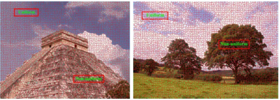
most existing methods use multiple features as a combined vector for matching, which implies that individual features contributeequallyto region matching across the entire image. However, a specific type of feature is often more effective for certain types of regions. It is thus beneficial to treat regionsdifferentlyaccording to their local charac-teristics. For example, pixels in uniform regions are more suitable to be matched by
20
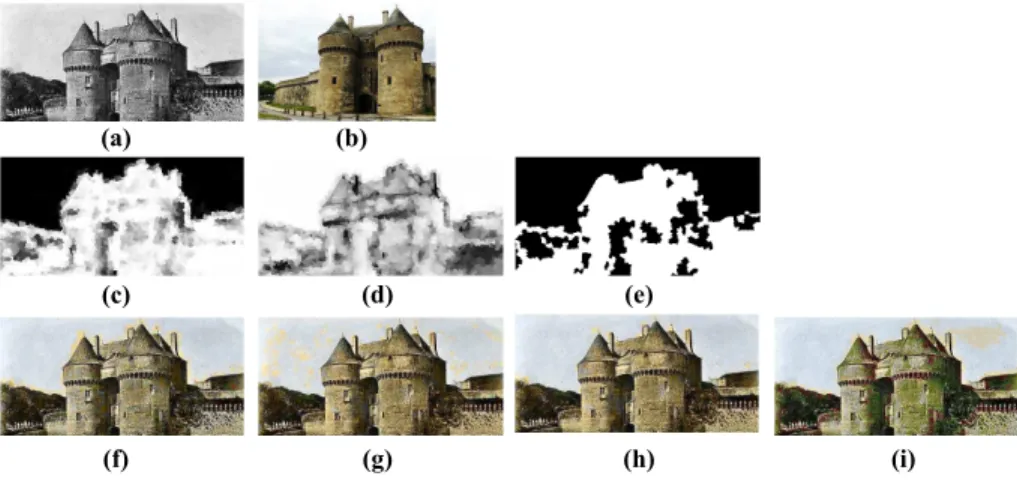
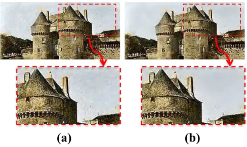
intensity features whereas texture descriptors should be used for highly non-uniform regions. An example is shown in Fig. 1. We can see that the intensity feature is suitable for the sky region but not the castle (Fig. 1(f)), whereas the texture descriptor performs well for the non-uniform castle regions but produces erroneous matches in the uniform
(a) (b)
(c) (d) (e)
(f) (g) (h) (i)
Figure 1: Illustration of automatic feature selection for colorization. (a) target grayscale image, (b) reference color image, (c)(d) probability maps of uniform and non-uniform regions (black to white for 0 to 1), (e) the optimal label image learned by an MRF model (black: uniform, white: non-uniform), (f)(g): colorization re-sults using intensity feature and SURF texture feature respectively, (h) colorization result using our proposed automatic feature selection and fusion, (i) the result using direct combination of intensity and SURF texture features.
regions (Fig. 1(g)). Combining these two features improves the result (Fig. 1(i)), but
25
numerous matching errors remain which lead to the green tint on the castle and the yel-low tint in the sky. Our automatic feature selection and fusion is effective at avoiding such problems (Fig. 1(h)).
In this paper, we propose a novel image colorization method via automatic fea-ture selection within a Markov Random Field (MRF) framework. To the best of our
30
knowledge, this is the first work that exploits automatic feature selection and fusion for image colorization. Specifically, image regions can be generally classified as being uni-form or non-uniuni-form. In uniuni-form regions, the luminance of pixels is evenly distributed, so the intensity distribution can represent these regions well, whereas in non-uniform regions, texture feature descriptors are effective to represent the patterns. Based on
35
the learned distribution of intensity deviation for uniform and non-uniform regions, the probability of a given region being assigned a uniform or non-uniform label is es-timated using Bayesian inference, which is then used for selecting suitable features. Instead of making individual decisions locally, we further develop an MRF model to
improve the labeling consistency where the probability is used for the label cost and
40
similarity between the luminance of the neighboring regions for the smoothness cost. The MRF model can be efficiently solved by the graph cut algorithm, enhancing the lo-cal consistency of the colorization result. Finally, the colorization results are obtained by transferring corresponding chrominance information from the reference image to the target grayscale image.
45
The main contributions of the paper are summarized as follows: 1) We propose a novel approach to improving image colorization by local feature selection and fusion. 2) We develop a novel algorithm that classifies local image regions into uniform and non-uniform regions and applies suitable features. An MRF framework guided by Bayesian probability inference is further proposed to improve locality coherence. 3)
50
We perform extensive experimental analysis both visually and quantitatively, which shows that the proposed method outperforms state-of-the-art methods.
The rest of this paper is organized as follows. We review work most relevant to this paper in Sec. 2, and then describe the proposed algorithm in detail in Sec. 3. Experi-mental results are shown in Sec. 4 and finally conclusions are drawn in Sec. 5.
55
2. Related Work
In general, existing image colorization methods can be divided into three cate-gories: user-scribble based methods, example-based methods and methods that use a large number of training images. User-scribble based methods are semi-automatic, and they often require substantial user interaction as input. In the pioneering work by Levin
60
et al. [8], some color scribbles on the target image are required as input, and then the color will be propagated based on least squares diffusion. However, there are obvious color bleeding effects around edges due to the isotropic nature of the diffusion. In order to better preserve the edge structure, an adaptive edge detection based colorization al-gorithm was proposed in [9]. To make the color region boundaries more consistent with
65
human judgement, a saliency guided colorization technique was proposed in [10]. The approach first generates a saliency map of the reference and target images to predict the visual attention of human viewers, softly segmenting the images into foreground and
background regions. Color transfer is then performed first to the foreground and then the background using a weighted color transfer algorithm. In [11], a fast colorization
70
method based on the geodesic distance weighted chrominance blending was proposed. Thanks to the use of luminance-weighted chrominance blending model and efficient intrinsic distance computation, the method is efficient for both image and video col-orization. However, for all these scribble-based methods, it is time-consuming and the quality of colorization results highly depends on the appropriateness of user scribbles.
75
Compared with user-scribble based methods, example-based methods can be fully automatic without any user interaction. For example-based methods, typically only one reference image with color information is needed, and the target grayscale image is colorized automatically. The pioneering work by Welsh et al. [4] first finds the best matching sample in the reference image for each pixel in the target image, and
80
then the chrominance information is transferred to the target grayscale image from the color reference image by the matching results to form the colorized images. Most of the existing example-based colorization algorithms follow this framework involving the steps of feature matching and color transfer. As feature matching is critical to the quality of results and the proposed method, Welsh’s method resorts to manually
85
specified swatches when automatic matching fails to produce satisfactory results. In order to improve the feature matching performance, different features or different combinations of features have been proposed. Ying et al. [12] proposed using a more extensive neighborhood descriptor computed using co-occurrence matrix based texture features. To reduce artifacts caused by outliers, the edit-nearest-neighbor method [13]
90
is used to try to remove the outliers. While the paper presents examples showing im-proved results, the co-occurrence matrix is expensive to compute. Chen et al. [14] combined [4] with foreground/background image matting to improve the colorization results but user interaction is needed to guide the grayscale image matting. Most of the existing methods focus on finding a proper combination of features for thewhole
im-95
age, rather thanselectingproper features for each local pixel or region, as we propose to do in this paper.
As the methods above match each pixel in isolation, spatial consistency cannot be guaranteed in general. In order to enhance locality consistency and reduce color
Target gray image
Reference
Reference
Result
Result Result by deep network[21]
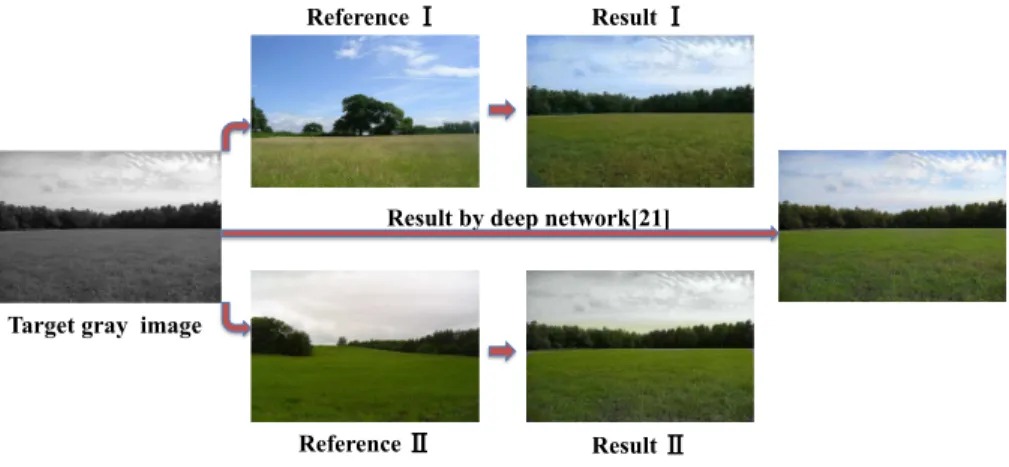
Figure 2: Colorization results with different reference images. While all the colorized images look plausible, our method is able to produce different colorized images based on different reference images. In comparison, deep learning based method [18] can only produce one output.
bleeding effects at edges, an edge-preserving total variation based image colorization
100
algorithm was proposed in [15]. However, since only chrominance information is in-volved in the variational formulation, the results of [15] suffer from halo effects near strong contours. In [16], a coupled regularization term with luminance and chromi-nance channels is introduced to preserve image contours during the colorization pro-cess. The method produces colorization results which are better aligned with edge
105
structures. However, significant artifacts can still be produced by incorrect feature matching. Compared with the local matching based methods, a novel global coloriza-tion method based on histogram regression was proposed in [17]. The basic assumpcoloriza-tion is that the final colorized image should have a similar color distribution as the reference image, and color matching is conducted by finding and adjusting the zero-points of the
110
color histogram. The method however may not work well for complicated scenarios where the color mapping cannot be effectively represented using global histograms.
An alternative category of approaches resorts to a large number of training images. For example, the proliferation of internet images can be utilized for image coloriza-tion. In [19, 20, 21], target grayscale images are colorized by internet images. The
115
Target grayscale image
Reference color image Superpixel segmentation and feature extraction
Optimal feature selection by MRF Multiscale Voting
Intensity guided color propagation
Figure 3: The pipeline of the proposed method.
the user and from the vast number of returned images a subset is chosen by means of a combined similarity metric. However, it is computationally expensive and depends on the accuracy of the semantic segmentation. Recently, deep learning based methods have been proposed for image colorization [6, 7, 18, 22] and produce promising results.
120
However, unlike example-based methods, the colorization results cannot be controlled by users. Since image colorization is essentially an ill-posed problem: the target im-ages can often be naturally colorized in different ways due to semantic ambiguities and style preference. One example is shown in Fig. 2. We can see that given different style reference images, our method, as an example-based method, can generate multiple
dis-125
tinct and plausible colorization results (e.g. the sky can be blue for a sunny day or gray for a cloudy day), while the recent deep learning based method [18] does not provide flexible control and can only produce one output image.
In this paper, a novel example-based image colorization method is proposed. Un-like existing methods, we aim to automatically find suitable features for each local
130
region rather than using the same feature for the whole image globally. We further pro-pose an MRF framework to solve feature selection and locality consistency simultane-ously, which can be efficiently solved using the graph cut algorithm. As we will show later, our automatic feature selection helps to significantly improve feature matching,
and thus provides an effective solution to a major challenge of image colorization.
135
3. Our Method
The pipeline of the proposed algorithm is shown in Fig. 3. In order to suppress the influence of global luminance difference between the reference and target images, a global linear luminance remapping to the reference image is applied as in [4]. For computational efficiency, and to help improve the spatial consistency of the results,
140
both the reference and target images are segmented into superpixels, and intensity and texture features are extracted from each superpixel. Using either of these features, we can find the corresponding best matching result for each target superpixel based on the Euclidean distance in the feature space (efficiently computed using the ANN library [23]). Then a two-label MRF model is formulated to choose the optimal
cor-145
respondence according to different features, based on the probability of superpixels belonging to uniform or non-uniform regions. Following the initial labeling, a multi-scale voting process is performed to eliminate the isolated outliers and enhance locality consistency. Finally, the chrominance channels are filtered by the standard guided fil-ter [24] with the guidance of the luminance channel.
150
3.1. Image Segmentation and Feature Extraction
For example-based image colorization, the most time-consuming step is finding the correspondence from the reference color image for each pixel in the target grayscale image. It is computationally expensive, especially when the feature dimensionality is high. On the other hand, neighboring pixels in natural images often share similar
char-155
acteristics, and can be processed simultaneously and in the same manner. As we will demonstrate later, doing so also ensures coherent colorization in local neighborhoods and reduces mismatches. Based on the above observation, both the reference image and the target grayscale image are first segmented into superpixels. For the reference image, superpixel segmentation is performed using the color information, whereas the
160
target grayscale image is segmented using the luminance information only. In this pa-per, we adopt the Turbopixel algorithm [25], which can process color and grayscale
Figure 4: Examples of superpixel segmentation shown with magnified selection.
images while preserving the edge structure well. The superpixel number is set to4000 in our experiments which provides a good balance between efficiency and quality, as we will demonstrate later. Note that the required number of superpixels depends on
165
the image content, rather than its resolution. Fig. 4 shows the superpixel segmentation results for both color and grayscale images. From the magnification of the boundary areas, we can see that the edge structure is well preserved.
For each superpixel from the reference color image and the target grayscale image, two types of features are extracted:
170
Intensity feature. The intensity feature we used is a 27-dimensional vector computed based on the luminance value. It is composed of three parts: the mean intensity within the superpixel (¯l1), the mean intensity of the neighboring superpixels (¯l2) and the
in-tensity distribution within the superpixel (hl), where¯l2= 1
|Ni|
P
j∈Ni ¯
l1(j)andNiis the set of neighboring superpixels of theithsuperpixel. The intensity distributionhl 175
is a histogram of the intensity distribution within each superpixel. In our experiments, the intensity range0–255is divided into 25 bins, and each entry represents the propor-tion of the pixels whose the intensity is in the range of the bin compared with the total number of pixels in the superpixel. The intensity feature is denoted asfI.
Texture feature. In this paper, the scale-invariant and rotation-invariant SURF
fea-180
ture [26] is used as the texture descriptor. At each pixel a 128-dimensional SURF descriptor is extracted, and then the average SURF feature within the superpixel is computed as the texture feature of the superpixel. We denote the texture feature asfT. These intensity and texture features are chosen because they are representative for their feature types and produce competitive results (see also the comparative results
185
between our method and state-of-the-art methods). Since the focus of this paper is novel feature selection and fusion, these elementary features are fixed, although our method can be directly combined with alternative features. To help choose intensity or texture feature for matching, the intensity standard deviationdiwithin each superpixel
iis also computed. A small value of the standard deviation implies that the intensity
190
distribution within the superpixel is even. The standard deviation is used for automatic selection of features (see the next subsection for detail), rather than finding the best candidate.
Figure 5: Examples of training samples from uniform and non-uniform regions.
3.2. MRF-based Automatic Feature Selection
In this subsection, we discuss our novel automatic feature selection for image
col-195
orization. The intuition is that different regions can be better represented by different features. In general, a natural image can be decomposed into uniform and non-uniform regions. We use the term non-uniform in a broad sense to refer to regions containing sufficient details, to allow texture descriptors to work effectively. This is different from
(a) uniform regions (b) non-uniform regions
Figure 6: The histograms of standard deviation of superpixels extracted from uniform and non-uniform training examples, and their fitted Gamma distributions.
the standard texture/non-texture classification [27, 28] so we develop a simple approach
200
for our purpose. In uniform regions, the luminance of pixels is evenly distributed, and the intensity featurefI can represent these regions well. While in non-uniform regions,
texture feature descriptorsfT are a good choice to represent repeated patterns. One of the main contributions of this paper is to design an automatic feature selection frame-work for each superpixel within an MRF frameframe-work. In addition to feature selection,
205
locality consistency can also be simultaneously enhanced by the MRF model.
3.2.1. Probability Estimation for Region Uniformity
When the superpixel segmentation is dense enough, the intensity standard deviation of each superpixel can be seen as a good descriptor to determine its characteristics, i.e. smaller deviation implies uniform while bigger value means non-uniform. Therefore
210
we adopt intensity standard deviation as the feature variable to estimate the probability distribution of each type of region.
In this paper, Bayesian inference is used to determine the probability of each super-pixel belonging to each type of region. For theithsuperpixelxi, given its correspond-ing standard deviationdi, we denote its probability of belonging to a uniform region as
P(xi ∈ U|di). Using Bayesian inference, the posterior probability can be computed by
P(xi∈U|di) =
P(U)P(di|xi∈U)
P(U)P(di|xi ∈U) +P(N)P(di|xi ∈N)
whereP(U)(orP(N)) denotes the a priori probability for a region to be uniform (or non-uniform), andP(di|xi ∈U)(orP(di|xi ∈N)) is the conditional probability of having given standard deviationdifor a region known as uniform (or non-uniform). In 215
general, we assume uniform and non-uniform regions are equally common and the a priori probabilitiesP(U),P(N)can be set as 0.5.
In order to estimate the conditional probabilityP(di|xi ∈U)andP(di|xi ∈N), we create a training set by manually selecting superpixels from uniform and non-uniform regions, and calculating the corresponding standard deviation values. In this paper, we collected 3000 superpixels for each type of region from 10 images, which are sufficient to estimate the distributions of standard deviation. An example is shown in Fig. 5. The histograms of the standard deviation for uniform and non-uniform regions are shown in Fig. 6. The shape of the histogram can be well approximated by a Gamma distribution
Γ(α, β) = β
αxα−1e−xβ
Γ(α) (2)
whereαandβare the shape and scale parameters of the Gamma distribution. Given our training samples, the Gamma distributions fitted are shown in Fig. 6, with the parameters for uniform regions and non-uniform regions being:{αU = 0.9544, βU = 220
2.3424}and{αN = 2.8295, βN = 9.8095}.
Given a superpixel with luminance standard deviationdi, its probability of belong-ing to uniform regionsP(xi ∈U|di)can be computed using Eqn. 1. We can similarly compute its probability of belonging to non-uniform regionsP(xi ∈ N|di), which satisfiesP(xi ∈ U|di) +P(xi ∈ N|di) = 1. The probability of uniformity is also 225
useful for feature matching as uniform regions should generally be colorized using samples from uniform regions, and the same for non-uniform regions. We thus add
P(xi ∈ U|di)to each type of the features introduced in the previous section which serves as a soft constraint.
3.2.2. MRF-based Labeling for Feature Selection 230
With the estimated posterior probability, a trivial way of labeling superpixels as uniform or non-uniform is thresholding. Such approach however does not take into ac-count spatial consistency. In this paper, we propose a novel automatic feature selection
approach for image colorization within an MRF framework. For each superpixel in the target image, we can find two matched superpixels from the reference image based on
235
the intensity and texture features. The searching process can be efficiently performed using the approximate nearest neighbour (ANN) tree searching algorithm [23]. An ex-ample is shown in Fig. 1. We can see that the intensity features perform well within uniform regions (Fig. 1(f)), whereas the texture descriptor is effective at non-uniform regions (Fig. 1(g)). Most existing methods combine these two types of features as
240
a combined feature and use the same searching process in both cases. The result as shown in (Fig. 1(i)) still contains many incorrect matching results. Rather than com-bining the two features, in this paper we assume that for each superpixel the matching result is determined by only the single optimal feature. We assume that in uniform regions the colorization should be determined by the intensity feature, whereas in the
245
non-uniform regions the texture feature should be dominant. Therefore, the problem of feature selection can be regarded as a binary labeling problem, where label0denotes intensity feature and label1means texture feature.
Let us denote the i-th superpixel in the target image asxi, and the set of all su-perpixels in the target image asΩ. N represents the set of adjacent superpixel pairs. The task of feature selection is to divide the whole setΩinto two disjoint sets, ΩI for regions determined by intensity features andΩT for regions determined by texture features. The binary labeling problem can be formulated as the minimization of the following MRF energy function
min S E( S) =X i∈Ω D(Si) +λ X (i,j)∈N f(Si, Sj), (3)
whereSiis the label for thei-th superpixel, which takes0or1to indicate whether the intensity feature or the texture feature is selected.
250
The first termD(Si)is the label cost which measures the cost to assign labelSi to thei-th superpixelxi. Based on our assumption, the label cost of each superpixel should be determined by its probability of belonging to either the uniform regions or
non-uniform regions, i.e. the posterior probabilities: D(Si) = P(xi∈N|di) ifSi= 0, P(xi∈U|di) ifSi= 1. (4)
The second termf(Si, Sj)is the pairwise term, which indicates the cost for assign-ing labelSito thei-th superpixels while assigning labelSj to thej-th superpixel. In this paper, the pairwise term is defined as
f(Si, Sj) = 0, ifSi=Sj s(i, j), otherwise (5) wheres(i, j)describes the similarity between adjacent superpixels. For improved co-herence, we assume that neighboring superpixels with similar intensity values are likely to have the same label. Therefore, the functions(i, j)is defined as follows:
s(i, j) = exp ( −kci−cjk 2 2σ21 ) exp −(¯l1(i)−¯l1(j)) 2 2σ22 , (6)
whereciand¯l1(i)are the central location and the mean intensity of thei-th superpixel.
σ1, σ2are parameters set asσ1 = 100andσ2 = 1(for images with approximately 1
megapixels). From the definition, the pairwise costs only exist for adjacent superpixels with different labels, and the effect is determined by the similarity between superpixels: i.e., the cost will be big if different labels are assigned to nearby superpixels with
255
high similarity. Therefore, the main effect of the pairwise term is to enhance locality consistency, which is important for colorization.
Given the label cost and the pairwise terms, the two-label MRF model (3) can be optimized by the graph cut algorithm [29, 30]. Since our energy function is not sub-modular, the alpha-beta swap algorithm is adopted, which randomly selects two
260
labels from the label set and tries to reduce the energy by swapping these labels. The algorithm is efficient, and runtime is less than 0.1 s for 4000 superpixels.
Finally, feature selection is determined by the labeling. For regions with label0, i.e., uniform regions, the intensity feature is used for feature matching. Otherwise, the texture feature is used. Fig. 1 shows the colorization result by the proposed
fea-265
feature and the texture feature. (f) and (g) are the corresponding best matches using intensity and texture features, respectively. (e) is the optimal labeling obtained by the MRF model and (h) is the final colorization result. Our feature selection performs sig-nificantly better than using individual features, or their simple combination as shown
270
in (i).
3.3. Consistency enhancement by multiscale voting
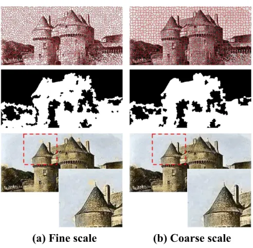
Although locality consistency has been taken into account in the MRF energy func-tion, there still exist isolated wrong matches as shown in Figure 7(a). In order to improve the color consistency, a multiscale voting is further performed. The basic
in-275
tuition is that the label assignment for a superpixel is likely to be wrong if most of its neighboring superpixels with similar image properties are assigned another label. Therefore, we can exploit neighboring superpixels to identify and correct invalid label assignments.
The target image is also oversegmented to produce coarse-scale superpixels by the
280
Turbopixels method. In this paper, the number of coarse-scale superpixels is chosen as a quarter of the original superpixel segmentation. For each superpixel in the coarse scale, the final label is determined by the majority label obtained in the fine scale. Finally, median filtering is applied for the chrominance channels in the lab color space such that the color of each superpixel is replaced by the median of its neighboring
285
superpixels, to further enhance color consistency. The result of multiscale voting is shown in Fig. 7(b). From the magnified selection, we can see that many isolated wrong matches are corrected.
3.4. Color propagation by guided filter
Although the multiscale voting process can reduce isolated matching errors, the
re-290
sulting color images still show block effects as chrominance information is transferred on a superpixel basis, and can have quite a few sparse outliers, as shown in Fig. 8(a). Different from other image processing tasks, the target grayscale image is accurate for image colorization. Therefore, the intensity information of the target image can be
(a) Fine scale
(b) Coarse scale
Figure 7: Example of multiscale voting. (a) fine scale matching without multiscale voting, (b) result with multiscale voting. From top to bottom: fine and coarse scale superpixels, uniform/non-uniform labels with-out and with multiscale voting, and colorization results withwith-out and with multiscale voting.
(a)
(b)
Figure 8: Example of luminance guided image filtering. (a) the original matching result, (b) the result after guided image filtering.
used to enhance the results, by exploiting the fact that nearby pixels with similar
in-295
tensity values should come with similar colors. For this purpose, we adopt the guided filter [24] for color propagation where the target grayscale image is used as guidance, which is an edge-preserving smoothing operator which better utilizes the structures in the guidance image.
J∗=X j
Wij(I)Jj (7)
whereImeans the target grayscale image which is used as the guidance image, Jis 300
the obtained chrominance channel from the last step, andWis the adapted weight
function as defined in [24]. The filtered image is shown in Fig. 8(b). We can see that block effects are smoothed while the edge information is preserved well.
4. Experiments
In this section, experimental results are presented to evaluate the performance of the
305
order to make a fair comparison, the results of [17] are generated using the code pro-vided by the author, and the results of [15] and [16] are propro-vided by the authors. The results of different algorithms are evaluated both by visual inspection and by quantita-tive evaluation. In addition to example-based methods, two of the latest deep learning
310
based methods [18, 22] are also included for visual comparison, using the code pro-vided by authors. Since the standard quantitative measures we used to compare the results are not designed for the task of image colorization, in order to get fair and reli-able comparison, a user study is also performed. The experiments were carried out on a computer with an Intel i7 2.8GHz CPU and 16GB memory.
315
4.1. Visual inspection
Thirteen natural images of different types, e.g., landscape, animals, and buildings, are chosen for the experiment. The colorization results are shown in Fig. 9. In order to evaluate the performance of automatic feature selection, the colorization results us-ing the combined intensity and texture features are also presented as a baseline. From
320
visual inspection, we can see that in most cases the proposed algorithm achieves the best results compared against the other four methods. In particular, our method sub-stantially reduces wrong color matches, especially between uniform and non-uniform regions.
Method [17] is based on finding and adjusting the zero-points of the histograms of
325
both the reference and target images. While less likely to be affected by local content, the global mechanism can result in mismatches within large regions when the zero-point based correspondence contains errors (see the 1st, 3rd and 4th rows of Fig. 9). Both the methods [15] and [16] solve the image colorization problem by automati-cally selecting the best color among a set of color candidates via a total variational
330
framework. Method [15] only retains the U and V channels without coupling of the chrominance channels with the luminance, and as a result their regularization algo-rithm creates halo effects near strong contours, as shown in the 1st, 4th, 7th and 11th rows of Fig. 9. In [16], a strong regularization coupling the luminance and chromi-nance channels is proposed to preserve the structural information of the image during
335
target reference [17] [15] Combined feature
proposed [22] [18] [16]
Figure 9: Comparison of our colorization results with alternative methods. From left to right: target and reference images, and the results of different methods.
[17]
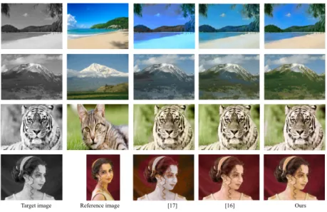
Reference image [16] Ours Target image
Figure 10: Comparison of our colorization results with alternative example-based colorization methods.
improvement over the method [15]. However, wrong matches remain for challenging scenarios (e.g. 1st-3rd rows of Fig. 9). The sixth column shows the results generated with trivially combined intensity and texture features. We can see that there are numer-ous incorrect matches, e.g., the green grass is mistakenly matched to the blue sky in the
340
2nd row of Fig. 9, and the uniform gray sky is mistakenly matched to the grass in the 3rd row of Fig. 9. In contrast, with automatic feature selection using our optimization framework, the proposed method improves color matching substantially and achieves better results as shown in the seventh column.
In addition to example-based methods, we also compare our colorization results
345
against the latest deep-learning based methods [18, 22]. Compared with example-based methods, the deep learning example-based colorization algorithms use millions of images for training the neural networks. In general, they can generate reasonable color images, as shown in the 8th and 9th columns of Fig. 9. However, there are some obvious artifacts shown e.g. in the 1st and 5th rows where parts of the meadow and elephant
350
are colored in blue. In addition, the output of such deep learning based methods cannot be controlled by the user.
varia-(a) Result generated by pixel (b) Result generated by superpixel
Figure 11: Colorization results by matching of pixels and superpixels.
tions are shown in Fig. 10. These examples are more challenging, as regions with sub-stantially different colors can have similar local characteristics in grayscale images. We
355
compare our results with state-of-the-art example-based colorization methods1. Due to the global mechanism of the method [17], it fails to reproduce correct colors from the reference images, as shown in the first two rows of Fig. 10. More specifically, it con-fuses the sand beach with the sea (first row) and grass meadow with the sky (second row), and produces large wrongly colored blue regions. It also generates obvious halo
360
effects around the boundary in the third row. The method [16] finds the optimal color matching using a variational framework. Thanks to the edge preserving capability of the variational function, [16] can reduce the halo effects around the boundary effec-tively. However, as only one type of feature is used to find the matching candidates, many obviously wrong colors are assigned. For example, in the first row, a large
por-365
tion of the beach is wrongly colored in blue as it is matched to the sky. This can be effectively avoided by using intensity feature in uniform regions as suggested in the proposed method. Similar problems can also be found in the remaining examples. In comparison, our method produces significantly better results than [15] and [16] for all of these cases.
370
1For this experiment, we compare with methods where code is publicly available, so the result of [15] is
Our method uses superpixels rather than pixels for matching. In this paper, an ap-proximate nearest neighbour (ANN) tree search algorithm is used to find the nearest match. ANN is computationally expensive when the feature dimensionality is high. For example, assuming both the reference image and the target image are of size300×400, for the 128-dimensional SURF descriptor, it takesover a dayto find matching pixels
375
by using the fast ANN algorithm2. In contrast, if the images are segmented into 4000
superpixels, the ANN algorithm just needs1.58s. In addition, neighboring pixels in natural images often share similar characteristics, so processing them simultaneously is not only substantially faster, but also improves local coherence and reduces the chance of mismatches. An example is shown in Fig. 11. To make pixel-based colorization
380
more tractable, we reduce the SURF feature dimension to 30 using PCA (Principal Component Analysis) which generally produces an output with similar quality. How-ever, the ANN step still takes863.82s, and the result is clearly less coherent than that with superpixels. Based on the above observation, both the reference image and the target grayscale image are firstly segmented into superpixels.
385
An additional experiment is designed to evaluate the influence of the number of superpixels. We choose the number of superpixels as 1000, 2000, 4000, 6000 and 8000, and apply our colorization algorithm. Fig. 12 shows the results with different number of superpixels and Table 1 shows the corresponding total running times, where both target and reference images are of the size300×400. It can be seen that when
390
the number of superpixels is too small, e.g., 1000, a superpixel may cover regions of mixed characteristics, which could result in a small number of mismatches. When the superpixel number is larger than 4000, the result is visually similar. However, the computational complexity and running times increase dramatically. In this paper, the number of superpixels is set to 4000 by default.
395
Table 1: The running times of our algorithm using different numbers of superpixels.
Number 1000 2000 4000 6000 8000
Time (s) 41.53 73.27 135.07 262.53 381.13
(d)
(b) (c) (e)
(a)
Figure 12: Colorization results with different numbers of superpixels. The first and third rows are the target and reference images. (a)-(e) in the second and fourth rows are the corresponding results with 1000, 2000, 4000, 6000 and 8000 superpixels.
4.2. Quantitative comparisons
In addition to visual inspection, we also make quantitive comparisons for the results shown in Figure 9. In this subsection, the results of deep learning methods [18, 22] are not included. On one hand, deep learning methods use millions of images for training while example-based methods take only one reference image. On the other hand, example-based methods generate results according to the given reference im-age, whereas the results of deep models are not controlled and thus can be irrelevant to the reference image. We thus focus on comparing our method with state-of-the-art example-based methods in the quantitative analysis to avoid misinterpretation. In this paper, we use the standard Peak Signal to Noise Ratio (PSNR) and Structural SIMilar-ity (SSIM) [31] as the measurements. Given anm×nground truth color imageu0and
the colorization resultu, PSNR (in db) is defined as
P SN R= 10·log10(
M AXI2
Table 2: The quantitative comparisons of different algorithms using the standard PSNR and SSIM measures. I–III are the corresponding results of methods [17, 15, 16], IV are the colorization results obtained by the combined features, and V are the results of the proposed feature selection method. 1–13: corresponding test images as shown in Fig. 9.
PSNR I II III IV V 1 20.91 16.01 21.63 20.71 24.71 2 22.66 17.40 22.68 20.91 24.49 3 21.03 17.97 24.88 24.03 25.61 4 20.28 17.09 26.92 23.58 23.19 5 23.38 22.65 24.31 21.36 22.39 6 24.39 22.39 24.55 18.18 23.49 7 19.78 14.94 21.84 20.84 23.02 8 18.37 17.89 18.82 18.37 18.91 9 20.17 16.26 18.35 18.07 19.598 10 23.93 22.75 31.12 25.15 23.50 11 14.33 13.06 14.04 14.31 14.38 12 19.76 19.61 20.33 18.40 24.42 13 23.06 20.36 25.51 24.59 23.89 SSIM I II III IV V 0.64 0.25 0.72 0.68 0.79 0.72 0.39 0.69 0.64 0.75 0.73 0.39 0.84 0.82 0.87 0.69 0.45 0.91 0.80 0.87 0.69 0.65 0.75 0.64 0.68 0.87 0.75 0.85 0.56 0.83 0.68 0.37 0.82 0.79 0.83 0.53 0.51 0.59 0.55 0.63 0.78 0.30 0.68 0.63 0.76 0.66 0.42 0.90 0.69 0.79 0.47 0.33 0.46 0.48 0.49 0.71 0.64 0.73 0.55 0.85 0.87 0.54 0.89 0.88 0.86
whereM AXI is the maximum possible pixel value of the image, which is 255 (with standard 8-bit samples). MSE is the mean squared error, which is defined as
M SE= 1 mn m−1 X i=0 n−1 X j=0 [u(i, j)−u0(i, j)]2. (9)
SSIM is designed to improve on traditional methods such as PSNR and MSE for better consistency with human visual perception. The scores for different algorithms are shown in Table 2. The quantitive measurements are generally in line with our visual inspection.
4.3. User study
However, since the standard measures are not designed for the task of image col-orization, in some cases, visually better results may get worse scores. For example, for the examples in 9th and 10th row of Fig. 9, the results of the proposed method appear more natural by visual inspection, but the PSNR and SSIM scores of our method are
405
lower than those of [16, 17]. Therefore, in order to make a fair comparison, we also perform a user study to quantitatively evaluate our method against other methods.
We designed the user study following the 2AFC (Two-Alternative Forced Choice) paradigm, which is widely used in psychological studies as it is both simple and reli-able. 200 users participated in the user study, with ages ranging from 18 to 38. For
410
each test image, every pair of results generated by the different algorithms is shown to the user and he/she is asked to choose the one of them, that looks better. To avoid potential bias, we randomize the order of image pairs shown to the user as well as their left/right position. We record the total number of user preferences (clicks) for each method, and treat these as random variables. The distribution of user preferences for
415
each method is summarized in Fig. 13. Note that since each method is compared with 4 alternative methods, and 13 examples were tested, the maximum number of user pref-erence for each method is 52. The one-way analysis of variance (ANOVA) is used to analyze the user study results. ANOVA is designed to determine whether there exist statistically significant differences between two or more independent groups. ANOVA
420
analysis gives the p-value for the null hypothesis that the means of the groups are equal. Smaller p-value means the groups are more significantly different.
In this paper, the p-values are computed between our method and each alterna-tive method. The results are shown in Table 3. It is clear that all of the p-values are very small which demonstrates the difference between our method and each alternative
425
method is statistically significant, based on the user study. From Fig. 13 we can see that majority of users prefer the method proposed in this paper (Fig. 13 V) which has the highest mean score.
Figure 13: Boxplots of user preferences for different methods, showing the mean (red lines), quartiles (blue lines), and extremes (black lines) of the distributions.
Table 3: The p-values of the ANOVA tests of the proposed method against other methods based on the user study results.
method I [17] II[15] III[16] IV (combined)
p-value 3.22e-30 2.05e-93 4.09e-38 1.43e-59
5. Conclusion
In this paper, we propose a novel approach to image colorization based on
auto-430
matic feature selection. By using suitable features for local regions based on their uniform/non-uniform characteristics, feature matching quality can be significantly im-proved, producing visually better colorization results. To achieve this, Bayesian infer-ence is used to estimate the label (type) of each region, and the optimization of feature selection is effectively formulated using a two-label MRF model. We further use
mul-435
tiscale voting and luminance guided image filtering to improve the consistency of the final colorization results. By feature selection, our method is able to produce coloriza-tion results better than individual features. However, both intensity and texture features used are low-level features and may fail to find semantically correct matches. Our
method can produce unsatisfactory results in case both features give wrong matches.
440
To address this, as the idea of using feature selection for improved image coloriza-tion is general, in addicoloriza-tion to the algorithm pipeline proposed in the paper, we would like to investigate automatic feature selection in alternative colorization frameworks e.g. by using more robust and semantically meaningful features, as well as for other applications such as color transfer.
445
Acknowledgements
We would like to thank the authors of [17, 18, 22] for providing their code, and the authors of [15, 16] for helping to generate comparative experimental results. This work is funded by natural science foundation of China (NSFC) 61262050, 61562062.
[1] S. A. Tsaftaris, F. Casadio, J.-L. Andral, A. K. Katsaggelos, A novel visualization tool
450
for art history and conservation: Automated colorization of black and white archival pho-tographs of works of art, Studies in Conservation 59 (3) (2014) 125–135.
[2] H. Chang, O. Fried, Y. Liu, S. DiVerdi, A. Finkelstein, Palette-based photo recoloring, ACM Transactions on Graphics (TOG) 34 (4) (2015) 139.
[3] Y. Chang, S. Saito, K. Uchikawa, M. Nakajima, Example-based color stylization of images,
455
ACM Transactions on Applied Perception 2 (3) (2006) 322–345.
[4] T. Welsh, M. Ashikhmin, K. Mueller, Transferring color to greyscale images, ACM Trans. Graph. 21 (3) (2002) 277–280.
[5] Y. Ling, O. C. Au, J. Pang, J. Zeng, Y. Yuan, A. Zheng, Image colorization via color propagation and rank minimization, in: International Conference on Image Processing,
460
IEEE, 2015, pp. 4228–4232.
[6] A. Deshpande, J. Rock, D. Forsyth, Learning large-scale automatic image colorization, in: Proceedings of the IEEE International Conference on Computer Vision, 2015, pp. 567–575. [7] Z. Cheng, Q. Yang, B. Sheng, Deep colorization, in: Proceedings of the IEEE International
Conference on Computer Vision, 2015, pp. 415–423.
465
[8] A. Levin, D. Lischinski, Y. Weiss, Colorization using optimization, ACM Trans. Graph. 23 (3) (2004) 689–694.
[9] Y.-C. Huang, Y.-S. Tung, J.-C. Chen, S.-W. Wang, J.-L. Wu, An adaptive edge detection based colorization algorithm and its applications, in: ACM Multimedia, ACM, 2005, pp. 351–354.
470
[10] N. Anagnostopoulos, C. Iakovidou, A. Amanatiadis, Y. Boutalis, S. Chatzichristofis, Two-staged image colorization based on salient contours, in: International Conference on Imag-ing Systems and Techniques (IST), 2014, pp. 381–385.
[11] L. Yatziv, G. Sapiro, Fast image and video colorization using chrominance blending, IEEE Trans. Image Processing 15 (5) (2006) 1120–1129.
475
[12] J. Ying, L. Ji, Pattern recognition based color transfer, in: International Conference on Computer Graphics, Imaging and Vision: New Trends, IEEE, 2005, pp. 55–60.
[13] F. J. Ferri, J. V. Albert, E. Vidal, Considerations about sample-size sensitivity of a family of edited nearest-neighbor rules, Systems, Man, and Cybernetics, Part B: Cybernetics, IEEE Transactions on 29 (5) (1999) 667–672.
480
[14] T. Chen, Y. Wang, V. Schillings, C. Meinel, Grayscale image matting and colorization, in: Proceedings of Asian Conference on Computer Vision, Citeseer, 2004, pp. 1164–1169. [15] A. Bugeau, V.-T. Ta, N. Papadakis, Variational exemplar-based image colorization, Image
Processing, IEEE Transactions on 23 (1) (2014) 298–307.
[16] F. Pierre, J.-F. Aujol, A. Bugeau, N. Papadakis, V.-T. Ta, Luminance-chrominance model
485
for image colorization, SIAM Journal on Imaging Sciences 8 (1) (2015) 536–563. [17] S. Liu, X. Zhang, Automatic grayscale image colorization using histogram regression,
Pat-tern Recognition Letters 33 (13) (2012) 1673–1681.
[18] R. Zhang, P. Isola, A. A. Efros, Colorful image colorization, in: European Conference on Computer Vision, 2016, pp. 649–666.
490
[19] A. Y.-S. Chia, S. Zhuo, R. K. Gupta, Y.-W. Tai, S.-Y. Cho, P. Tan, S. Lin, Semantic col-orization with internet images, in: ACM Transactions on Graphics (TOG), Vol. 30, ACM, 2011, p. 156.
[20] X. Liu, L. Wan, Y. Qu, T.-T. Wong, S. Lin, C.-S. Leung, P.-A. Heng, Intrinsic colorization, in: ACM Transactions on Graphics (TOG), Vol. 27, ACM, 2008, p. 152.
[21] X. Wang, J. Jia, H. Liao, L. Cai, Image colorization with an affective word, in: Computa-tional Visual Media, Springer, 2012, pp. 51–58.
[22] S. Iizuka, E. Simo-Serra, H. Ishikawa, Let there be color!: joint end-to-end learning of global and local image priors for automatic image colorization with simultaneous classifi-cation, ACM Transactions on Graphics (TOG) 35 (4) (2016) 110.
500
[23] D. M. Mount, S. Arya, ANN: library for approximate nearest neighbour searching. [24] K. He, J. Sun, X. Tang, Guided image filtering, IEEE Transactions on Pattern Analysis and
Machine Intelligence 35 (6) (2013) 1397–1409.
[25] A. Levinshtein, A. Stere, K. N. Kutulakos, D. J. Fleet, S. J. Dickinson, K. Siddiqi, Tur-bopixels: Fast superpixels using geometric flows, IEEE Transactions on Pattern Analysis
505
and Machine Intelligence 31 (12) (2009) 2290–2297.
[26] H. Bay, A. Ess, T. Tuytelaars, L. Van Gool, Speeded-up robust features (SURF), Computer Vision and Image Understanding 110 (3) (2008) 346–359.
[27] J. Li, J. Z. Wang, G. Wiederhold, Classification of textured and non-textured images using region segmentation, in: Proceedings of International Conference on Image Processing,
510
Vol. 3, IEEE, 2000, pp. 754–757.
[28] L. Costantini, L. Capodiferro, M. Carli, A. Neri, Textured areas detection and segmentation in circular harmonic functions domain, in: IS&T/SPIE Electronic Imaging, International Society for Optics and Photonics, 2012, pp. 829504–829504.
[29] Y. Boykov, O. Veksler, R. Zabih, Fast approximate energy minimization via graph cuts,
515
IEEE Transactions on Pattern Analysis and Machine Intelligence 23 (11) (2001) 1222– 1239.
[30] Y. Boykov, V. Kolmogorov, An experimental comparison of min-cut/max-flow algorithms for energy minimization in vision, IEEE Transactions on Pattern Analysis and Machine Intelligence 26 (9) (2004) 1124–1137.
520
[31] Z. Wang, A. C. Bovik, H. R. Sheikh, E. P. Simoncelli, Image quality assessment: from error visibility to structural similarity, IEEE Transactions on Image Processing 13 (4) (2004) 600–612.