Binary relevance efficacy for multilabel classification

(will be inserted by the editor)

Binary Relevance Efficacy for Multilabel Classification

Antonio Bahamonde

Received: date / Accepted: date

Abstract The goal of multilabel (ML) classification is to induce models able to tag objects with the labels that better describe them. The main baseline for ML classi-fication is Binary Relevance (BR), which is commonly criticized in the literature because of its label inde-pendence assumption. Despite this fact, this paper dis-cusses some interesting properties of BR, mainly that it produces optimal models for several ML loss functions. Additionally, we present an analytical study about ML benchmarks datasets, pointing out some shortcomings. As a result, this paper proposes the use of synthetic datasets to better analyze the behavior of ML meth-ods in domains with different characteristics. To sup-port this claim, we perform some experiments using synthetic data proving the competitive performance of BR with respect to a more complex method in difficult problems with many labels, a conclusion which was not stated by previous studies.

Keywords Multilabel Classification · Binary Rele-vance·Synthetic datasets·Label dependency

1 Introduction

Multilabel (ML) classification aims at obtaining models that provide a set of labels to each object, unlike multi-class multi-classification that involves predicting just a single class. This learning task arises in many practical do-mains; for instance, media documents (texts, songs and videos) are usually tagged with several labels to briefly inform users about their actual content. Another well-known examples include assigning keywords to a paper, Artificial Intelligence Center. University of Oviedo at Gij´on. Campus de Viesques, 33204, Gij´on (Asturias) Spain

www.aic.uniovi.es

illness to patients, objects to images or emotional ex-pressions to human faces.

ML classification has received many contributions from different points of view. In Schapire and Singer (2000) and Elisseeff and Weston (2001) the approach was an extension of multiclass classification. Other meth-ods follow different learning frameworks: this is the case of nearest neighbors (Zhang and Zhou, 2007), decision trees (Tsoumakas et al, 2010b), Bayesian learners (Za-ragoza et al, 2011; Bielza et al, 2011) and the combina-tion of logistic regression and instance based learning (Cheng and H¨ullermeier, 2009).

An interesting group of learners is based on the chain rule, using both inputs and labels in the learn-ing process. In this group are Read et al (2009b), Dem-bczy´nski et al (2010), and Monta˜n´es et al (2011). An-other successful approach consists in learning a ranking of labels for each instance and then, if necessary, pro-duce a bipartition with a threshold that can be a fixed value or a variable learned from the learning task, see Elisseeff and Weston (2001) and Quevedo et al (2012). Finally, there are other approaches that aim to explic-itly optimize a given loss function, for instance Dem-bczy´nski et al (2010), Dembczy´nski et al (2011), Pet-terson and Caetano (2010) and Quevedo et al (2012).

ML learning presents two main challenging prob-lems. The first one bears on the computational com-plexity of the algorithms. If the number of labels is large, then a very complex approach is not applicable in practice, so the scalability is a key issue in this field. The second problem is related with the own nature of ML data. Not only the number of classes is higher than in multiclass classification, but also each example be-longs to an indeterminate number of labels, and more important, labels present some relationships between them. From a learning perspective, the hottest topic

in ML community is probably to design new methods able to detect and exploit dependencies among labels. Actually, several methods have being proposed in that direction, for instance those based on the chain rule cited before.

Typically, all these new approaches are experimen-tally compared withBinary Relevance (BR) (Godbole and Sarawagi, 2004; Tsoumakas and Katakis, 2007), the main baseline for ML classification. BR is a decomposi-tion method based on the learning assumpdecomposi-tion that la-bels are independent. Therefore, each label is classified as relevant or irrelevant by a binary classifier learned for that label independently from the rest of labels. De-spite in those experimental studies BR is outperformed by new approaches, it should not be consider just as a mere baseline. This paper proves that BR is not only computationally efficient, which is important in many practical situations, but is also effective, in the sense that it produces good ML classifiers according to sev-eral metrics. In fact, BR is able to induce optimal mod-els when the target loss function is a macro-averaged measure. Moreover, this paper also supports the hy-pothesis that BR is competitive with respect to more complex approaches when the ML classification tasks are difficult, for instance, in domains with many labels and a high label dependency.

On the other hand, the experimental studies in ML classification have to deal with some issues. The most important one is the lack of rich collections of bench-mark datasets. Although ML is a very active area of re-search, there are only a few publicly available datasets. This fact conditions the experimental assessments of new proposals in such a way that some sophisticated algorithms seem to perform better than simpler learn-ers, like BR, only because of the experimental sampling. Having in mind this context, our proposal is to com-bine benchmark and synthetic datasets in order to ob-tain empirical evidences about the actual performance of ML methods in different learning situations. Usually, synthetic data have been employed to illustrate a par-ticular strength or weakness of a given algorithm, so in those cases the data generation process is algorithm-specific. In contrast, we propose to build tools that can produce synthetic datasets useful to study the behavior of any new ML classification method.

In this paper we employed a general-purpose gen-erator of synthetic datasets for creating a collection of ML problems that reproduce a wide variety of situa-tions. This generator1 _{produces synthetic ML data} al-lowing the user to select the desired values for some important characteristics, like the number of labels or the level of label dependency. Using a collection of syn-1 _{It is available online at www.aic.uniovi.es/ml generator.}

thetic datasets, we performed a exhaustive experiment comparing BR with an state-of-the-art method, ECC (Ensemble of Classifier Chains) (Read et al, 2011b). The results of these experiments show some interest-ing evidences that BR is very competitive in hard ML problems.

The main contributions of this paper are threefold: i) to formally discuss the properties of BR to obtain good models for macro-average loss functions; ii) to propose the use of synthetic datasets to remedy the shortcomings of benchmark datasets, and iii) to exper-imentally prove the competitive performance of BR in ML domains in which the number of labels and the label dependency are high.

The rest of the paper is organized as follows. The next section gives a formal presentation of ML learn-ing tasks and hypotheses. Section 3 reviews the main loss functions for ML classification. Then, we discuss the advantages of BR strategy, specially those related with its efficacy for optimizing macro-average loss func-tions. In Section 5 we present an analytical study about the properties of ML benchmark datasets. Next section describes a genetic algorithm to build ML synthetic datasets. Finally, Section 7 reports some experiments that support our claims and Section 8 draws some con-clusions.

2 Multilabel Classification

LetL be a finite and non-empty set of labels{l1, . . . , lL},

letX be an input space, and letY be the output space defined as the set of subsets of labelsL.

Definition 1 A ML classification task is given by a dataset

D={(x1,y1), . . . ,(xn,yn)} ⊂ X × Y (1)

of pairs of inputsxi∈ X and subsets of labels yi ∈ Y

as outputs.

The labels assigned to each input are usually referred to as therelevantlabels for the input entry.

Sometimes, when the input space is an Euclidean space ofpdimensions, we will refer to the learning task by a couple of matrices

D≡(X,Y), (2) in which X = (x1, . . . ,xn) and Y = (y1, . . . ,yn). In

order to make the notation clearer, each element ofY,

yij, is 1 when labelj is relevant for example i, and 0

otherwise.

The goal of a ML classification task D is to induce a hypothesis defined as follows.

Definition 2 AML hypothesisis a functionhfrom the input space to the output space, the power set of labels P(L); in symbols,

h:X −→ Y =P(L) ={0,1}L_{. (3)}

Hence, h(x) is the set of relevant labels predicted by

h for the object x. Sometimes, we use h(X) = Y to mean that the predictions ofhapplied to an input set represented by a matrix Xare a set of labels codified by a matrixY.

3 Loss Functions for Multilabel Classification ML classifiers can be evaluated from different points of view. The predictions can be considered either as a bi-partition or as a ranking of the set of labels. This paper only studies ML classification tasks. Consequently, the performance of ML classifiers will be evaluated as a bi-partition and the loss functions used must compare the subsets of relevant and predicted labels.

Usually this kind of measures can be divided in two main groups (Tsoumakas et al, 2010a). The example-basedloss functions compute the average differences of the actual and the predicted sets of labels over all ex-amples. The label-based measures decompose the eval-uation with respect to each label. There are two op-tions here, averaging the measure label-wise (usually called macro-average), or concatenating all label pre-dictions and computing a single value over all of them, themicro-averageversion of a measure. Macro-average measures give equal weight to each label, and are often dominated by the performance on rare labels. In con-trast, micro-average metrics gives more weight to fre-quent labels. These two ways of measuring performance are complementary one each other, and both are infor-mative.

For further reference, let us recall the formal defini-tions of these loss funcdefini-tions, given a ML hypothesis h

(3). For a predictionh(x) and a subset oftruly relevant labelsy⊂L, for each labell∈L we can compute the contingency matrix in Table 1.

Table 1 Contingency matrix for each label l∈_L given the actual relevant,y, and the predicted,h(x), labels

y[l] = 1 y[l] = 0 h(x)[l] = 1 a(x, l) b(x, l) h(x)[l] = 0 c(x, l) d(x, l)

Each entry (a, b, c, d) in this matrix has a value of 1 when the predicates of the corresponding row and column are both true, otherwise the value is 0. Notice

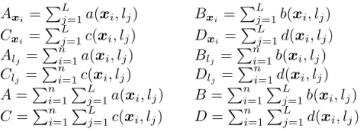
for instance, thata(x, l) is 1 only when the prediction of h includes the truly relevant label l. Furthermore, only one of the entries of the matrix is 1, the rest are 0. Throughout the definitions of the loss functions be-low, we will consider a set ofnexamples in a ML task withLlabels. Additionally, we use the following aggre-gations of contingency matrices:

Axi = PL j=1a(xi, lj) Bxi = PL j=1b(xi, lj) Cxi = PL j=1c(xi, lj) Dxi = PL j=1d(xi, lj) Alj = Pn i=1a(xi, lj) Blj = Pn i=1b(xi, lj) Clj = Pn i=1c(xi, lj) Dlj = Pn i=1d(xi, lj) A=Pn i=1 PL j=1a(xi, lj) B=P n i=1 PL j=1b(xi, lj) C=Pn i=1 PL j=1c(xi, lj) D=P n i=1 PL j=1d(xi, lj)

Definition 3 The Recall is defined as the proportion of truly relevant labels that are included in predictions. The example-based, macro and micro average versions are computed as follows:

Rex = 1 n n X i=1 Axi Axi+Cxi , Rma= 1 L L X j=1 Alj Alj +Clj , Rmi= A A+C.

Definition 4 The Precision is defined as the propor-tion of predicted labels that are truly relevant. Example-based, macro and micro versions are defined by

Pex = 1 n n X i=1 Axi Axi+Bxi , Pma= 1 L L X j=1 Alj Alj +Blj , Pmi= A A+B.

The trade-off between Precision and Recall is for-malized by theirharmonicmean, called F-measure.Fβ

(β≥0) is computed by

Fβ =

(1 +β2_)P·R

β2_P+R

Definition 5 Example-based, macro and microFβ(β≥

0) are defined by F_βex = 1 n n X i=1 (1 +β2_)A xi (1 +β2_)A xi+Bxi+β 2_C xi , F_βma= 1 L L X j=1 (1 +β2_)A lj (1 +β2_)A lj+Blj +β 2_C lj , F_βmi= (1 +β 2_)A (1 +β2_)A+B+β2_C. (4)

F1is the most frequently used F-measure.

Other performance measures for ML classifiers can also be defined using contingency matrices (Table 1). This is the case of theAccuracyandHamming loss. Definition 6 TheAccuracy(Tsoumakas and Katakis, 2007), or the Jaccard index, is a slight modification of theF1measure defined as

Acex= 1 n n X i=1 Axi Axi+Bxi+Cxi , Acma= 1 L L X j=1 Alj Alj+Blj +Clj , Acmi= A A+B+C.

Definition 7 The Hamming loss is the proportion of misclassifications. The macro-average is given by

Hlma= 1 L L X j=1 Blj+Clj Alj +Blj +Clj +Dlj . (5)

Taking into account that the sum of the components of contingency matrices (see Table 1) is 1, the macro Hamming loss can be written as

Hlma= 1 L L X j=1 Blj +Clj n = B+C L·n =Hlmi. Moreover, Hlma=Hlmi = 1 n n X i=1 Bxi+Cxi L =Hlex.

That is to say, the Hamming loss is a measure that has the same value in their macro, micro and example-based versions.

Finally, another important ML example-based met-ric is the Subset zero-one loss.

Definition 8 The Subset zero-one loss looks if pre-dicted and relevant label subsets are equal or not:

S0/1= 1 n n X i=1 [[yi6=h(xi)]]. (6)

in which the expression [[p]] evaluates to 1 if the pred-icate p is true, and to 0 otherwise. This metric is an extension of the classical zero-one loss in multiclass clas-sification, to the ML case.

4 Binary Relevance: a not so simple baseline BR is a straightforward approach to handle a ML clas-sification task. In fact, BR is usually employed as the baseline method to be compared with new ML meth-ods. It is the simplest strategy, but is more effective than it may seem at first sight.

BR decomposes the learning of h into a set of bi-nary classification tasks, one per label, where each sin-gle model hj is learned independently, using only the

information of that particular label and ignoring the information all other labels. In symbols,

hj :X −→ {0,1}.

The main drawback of BR is that it does not take into account any label dependency and may fail to predict some label combinations if such dependence is present. However, BR presents several obvious advantages: i) any binary learning method can be taken as base learner; ii) it has linear complexity with respect to the number of labels; and iii) it can be easily parallelized. But the most important advantage of BR is that it is able to optimizeseveralloss functions.

Given a ML classification task D (1), let M be a performance measure defined for a pair of lists of sub-sets of labels:

M (y1, . . . ,yn),(ˆy1, . . . ,yˆn)

=M(Y,Yˆ),

whereY and ˆYrepresent the lists of subsets of actual and predicted labels, respectively. If higher values ofM

are preferable to lower, then the optimal predictions for the list of inputsXare given by a hypothesis

h∗_M(X) = argmax ˆ Y X Y Pr(Y|X)·M(Y,Yˆ). (7)

It is straightforward to see that the optimization of macro-averaged measures is equivalent to the optimiza-tion of those measures in the subordinate BR classifiers. When M is a macro-averaged measure, the optimiza-tion of (7) can be decomposed through the set of labels. Thus, h∗_M(X) = argmax ˆ Y X Y Pr(Y|X)1 L L X j=1 M(Y[j],Yˆ[j]) = argmax ˆ Y X Y L X j=1 Pr(Y|X)M(Y[j],Yˆ[j]), (8)

in which,Y[j] is thejth_{column of matrixYthat}

repre-sents the corresponding label,lj. Notice that this

equa-tion holds for all macro-average measures defined in Section 3, including Hamming loss in any of its versions since they all are equal.

The consequence of (8) is that optimal predictions can be built from optimal outputs for each label for classification tasks drawn from the same distribution of the original ML task. That is, optimal BR classifiers will yield the optimal predictions.

Proposition 1 (Macro-average optimization). The op-timization of a macro-averaged measure M for a ML task can be accomplished by the optimization of the sub-ordinate BR classifiers for the binary version of M.

One consequence of this result affects the optimiza-tion of the Hamming loss, since it can be seen as the macro-average of the binary error rates of the labels (5).

Corollary 1 (Hamming loss optimization). The opti-mization of Hamming loss for a ML task can be ac-complished by the optimization of the subordinate BR classifiers for the binary error rate.

The same corollary can be stated for all other macro-average loss functions. To optimize such measures, the binary classifiers that compose a BR model must opti-mize the corresponding binary measure. For instance, the optimization of macroF1 requires that the binary classifiers optimize F1, using algorithms like the one proposed by Joachims (2005).

This section proves that BR is not just a baseline classifier, but it provides optimal models for several loss functions. For this reason, when new proposed ML learners are compared with BR using macro-averaged measures, the comparison must be done carefully, oth-erwise the derived conclusions may be biased. Another consequence is that future research in the field of ML classification should be focused on obtaining new the-oretically sound methods able to optimize other kind of loss functions, like example-based or micro-average measures.

5 Multilabel Benchmark Datasets

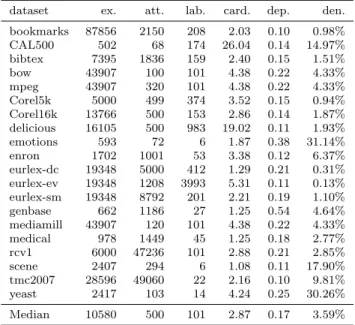
Despite the misuse of BR in comparative studies, there is another important issue when ML methods are an-alyzed empirically. The key problem is that there are just a few publicly available ML datasets. The most popular repository is maintained in MULAN website. MULAN (Tsoumakas et al, 2010a) is a WEKA exten-sion for ML. Table 2 reports the main properties of MULAN’s datasets.

In addition to the scarcity of datasets, it is surpris-ing that most of them are almost multiclass learnsurpris-ing tasks. This can be measured using thecardinality; that

Table 2 Description of MULAN datasets. For each dataset, the table shows the number of examples, the number of at-tributes, the number of labels, and the values for the cardinal-ity (9), unconditional label dependency (11) and denscardinal-ity (10). There are 10 different versions of Corel16k dataset in MULAN repository. We have only included one of them in this study because they have similar properties. The same happens with rcv1 datasets, with 5 distinct subsets. Tmc2007 dataset has another version with only 500 attributes, but again the rest of properties are practically the same

dataset ex. att. lab. card. dep. den. bookmarks 87856 2150 208 2.03 0.10 0.98% CAL500 502 68 174 26.04 0.14 14.97% bibtex 7395 1836 159 2.40 0.15 1.51% bow 43907 100 101 4.38 0.22 4.33% mpeg 43907 320 101 4.38 0.22 4.33% Corel5k 5000 499 374 3.52 0.15 0.94% Corel16k 13766 500 153 2.86 0.14 1.87% delicious 16105 500 983 19.02 0.11 1.93% emotions 593 72 6 1.87 0.38 31.14% enron 1702 1001 53 3.38 0.12 6.37% eurlex-dc 19348 5000 412 1.29 0.21 0.31% eurlex-ev 19348 1208 3993 5.31 0.11 0.13% eurlex-sm 19348 8792 201 2.21 0.19 1.10% genbase 662 1186 27 1.25 0.54 4.64% mediamill 43907 120 101 4.38 0.22 4.33% medical 978 1449 45 1.25 0.18 2.77% rcv1 6000 47236 101 2.88 0.21 2.85% scene 2407 294 6 1.08 0.11 17.90% tmc2007 28596 49060 22 2.16 0.10 9.81% yeast 2417 103 14 4.24 0.25 30.26% Median 10580 500 101 2.87 0.17 3.59%

is, the average number of labels per example. In sym-bols, the cardinality of a dataset is given by

cardinality(X,Y) = Pn i=1 PL j=1yi,j n . (9)

In the datasets of MULAN repository, the cardinality is very low; the median is just 2.87. Moreover, only 3 datasets out of 20 have a cardinality greater than 5, and 11 datasets have a cardinality lower than 3.

One important consequence of this fact is that the proportion of ones in the matrix Y of labels is also very low. This proportion is called the density of the dataset and it is defined as the cardinality divided by the number of possible labels,

density(X,Y) =cardinality(X,Y)

L . (10)

The median of the density in MULAN’s datasets, is only 3.59% (expressed as a percentage). Therefore, in some datasets a hypothesis predicting no labels for any input, will have a very low percentage of misclas-sifications. This is a good reason to carefully consider if the Hamming loss is as an appropriate performance measure for a given domain.

Nevertheless, the key ingredient that makes ML an interesting research problem is that the labels show

some kind of dependency between them. Otherwise, if the label independence assumption was fulfilled, BR would be the perfect approach. Thus, we need datasets with different levels of label dependency in order to evaluate the behavior of ML methods. Unfortunately, it is not trivial how to measure label dependency.

From a Bayesian point of view, there are two possi-ble kinds of dependency: the conditional and the uncon-ditional dependency (Dembczy´nski et al, 2010; Bielza et al, 2011; Zaragoza et al, 2011; Lastra et al, 2011). There areconditionaldependency between labels when-ever Pr(l1, . . . , lL|X)6= L Y j=1 Pr(lj|X).

This means that there are disjoint subsets of labels such that

Pr((lj :j∈J)|X)6= Pr((lj:j∈J)|X,(li :i∈I)).

On the other hand, the dependency between labels, if there is any, is unconditional when the reference to input variables of the above equations can be skipped. In this paper we measure this kind of dependency as the average of the correlation of labels weighted by the number of common examples. In symbols,

dependency(Y) = P i<jρ(li, lj)|li∩lj| P i<j|li∩lj| , (11)

in which ρ(li, lj) represents the absolute value of the

correlation coefficient between labelsli andlj.

Looking at the values of unconditional label depen-dency in Table 2, we see that half of the datasets have a label dependency in the range [0.1..0.15]. Only two datasets have a value greater than 0.25. It is quite evi-dent that the distribution of label dependency in MU-LAN’s datasets is not very diverse. Viewing these num-bers, how can one argue that a particular method is able to exploit label dependency if the experiments were performed using these datasets?

This brief analysis shows that the current collection of benchmark datasets presents important limitations. Specially, because ML problems are much more com-plex than those of other learning tasks, due to their own characteristics. For instance, in comparison with binary or multiclass classification, ML classification has addi-tional factors that are crucial, mainly the cardinality and the label dependency. This fact suggests that to study ML approaches experimentally we should need more datasets than for the same kind of experiment in the context of multiclass classification.

Our statement is that benchmark datasets do not provide enough support for the experimental study of

ML methods. For this reason, we propose to use them in combination with collections of synthetic datasets spe-cially devised to offer a wider range of characteristics. In the next subsection we describe one method that can be used to generate these collections.

6 A Generator of Synthetic Datasets

Strictly speaking, there are no generators of synthetic ML learning tasks published. The approach presented in Read et al (2009a, 2011a) is mainly concerned with streaming data and can hardly be used to obtain ML datasets with a realistic combination of the properties described in previous section.

To generate a ML dataset is not a trivial task. If one tries to concatenate several binary classification tasks with the same input instances, the result is that the labels will have no relationship at all. But, as we stated before, it is mandatory to obtain some kind of depen-dency among labels.

In this paper we used a genetic algorithm2_{to search} for ML datasets with a set of target characteristics se-lected by the user. The goal is to obtain, for each desired combination of properties, three datasets: train, valida-tion and test, with approximately the same properties values. They will be represented by matrices as in (2).

6.1 Data Generation

In all cases, the input space will be a hypercube

X = [0,1]p ⊂Rp. (12)

The requisites of the search set by the user include: number of labels, number of examples for test, training and validation sets, cardinality and dependency.

All parameters but cardinality and dependency are somehow structural and can be easily fulfilled. Thus, the generator starts with a set of inputs drawn from a uniform distribution inX; letXbe the matrix of input instances for the training set. The core idea of the gen-erator presented here is that it searches for ahypothesis to classify the inputs inXand obtain a ML task with cardinality and dependency as close as possible to those specified by the user.

Once the hypothesis is found, the validation and test datasets are built; their input instances are inde-pendently drawn with uniform distribution again, from the input spaceX. This guarantees that training, vali-dation and testing examples come from the same distri-bution and the properties of these sets are more or less

the same. Or stated differently, these sets will have ap-proximately the same values for features like cardinality and label dependency.

Thus, the focus of the generator are the hypotheses for ML classification. These hypotheses are formed by a group of hyperplanes that split the input space in a positive and a negative region. In fact a set of hyper-planes may define a linear classifier or a nonlinear one. We build nonlinear tasks in this work.

For this purpose, we assign relevant labels to regions of the input space defined by the intersection of several hyperplanes that share a common point. In other words, the relevant labels are geometrically defined at the in-terior of pyramids with a certain number offaces. In all cases,

X = [0,1]p.

Then, for a given labellj, we define a hypothesishj as

follows: hj(x) = 1 ⇐⇒ hwkj,x−x 0 ji ≥0, ∀k= 1, . . . ,faces. where x0_j ∈ X,wk_j ∈[−1,1]p, k= 1, . . . ,faces.

However, if the list of vectorswk

j is completely

ran-dom, the interior of the pyramid may be empty or too small. To avoid these possibilities we force the list ofwk_j to form angles within a given range, using the following procedure. First, a set of vectors (wk

j :k= 1, . . . ,faces)

is randomly drawn in [−1,1]p. Then, using the Gram-Schmidt procedure, we obtain an orthonormal basis of the linear span of vectorswk

j. Let

(vk_j :k= 1, . . . ,faces)← Gram-Schmidt(wk_j :k= 1, . . . ,faces)

If the rank of vectorswk_j is not equal tofaces, a new set is drawn. The next step redefines the vectors of the nonlinear hypothesis as follows:

w1j ←v1j wk_j ←λv1_j+vk_j, k= 2, ...faces Notice that cos(w1_j,wk_j) = hv 1 j, λv1j+vkji √ 1 +λ2 = λ √ 1 +λ2 Therefore, cos2_(w1 j,wkj) 1−cos2_(w1 j,wkj) = 1 tan2(w1 j,wkj) =λ2

and hence it is straightforward to fix a range forλvalues if we want that, for instance,

angle(w1_j,wk_j)∈[50o,80o],∀k= 2, . . . ,faces.

Notice that the interior angle of pyramid faces with the first one will range in [100o_,130o_{]. In the experiments} reported at the end of the paper, the number of faces will be set to 5.

6.2 Conditional Dependency

To obtain a dataset with a certain degree ofconditional dependency, we can use the following method of two steps. IfLis the number of labels required, first we use the procedure described above to search for a dataset withL/2 labels. Let

D1= (X,YL/2)

be such a dataset. Thus, to obtain the rest of labels, we use the whole datasetD1as the input instances and search for a new collection ofL/2 labels. In this way we have

D2= (X,YL/2),Y0L/2

.

At the end, we obtain

D= X,

YL/2YL/0 2

,

a dataset withLlabels and some degree of conditional dependency.

To ensure a cardinality similar to a given amount set by the user, we divide the cardinality in two equal parts: one part for the matrixYL/2 searching for D1, and the rest for the second half for the matrix, Y0_L/2, searching forD2.

On the other hand, the unconditional dependency can not be guaranteed. Thus, we ask for the same amount in both searches in order to reach a similar value at the end of the process.

7 Experiments

Several experimental studies in the literature based on benchmark datasets, see for instance Read et al (2011b) and Monta˜n´es et al (2011), report a better performance of new ML methods with respect to BR in terms of some loss functions, including macro-average measures. Most of these new approaches are aimed at exploiting label dependency. The conclusion of these studies is that the improvement is due to overcoming the main drawback of BR, the label independence assumption.

However, as we previously discussed on Section 5, benchmark datasets are somehow limited in several as-pects. The main idea of our experiments is to make a broader comparison between BR and a recent ML method. The aim is to prove if the better performance

of this new ML learner on benchmark datasets still re-mains in other dore-mains, in which we can control some important properties for ML classification, such as the number of labels, the cardinality and, more importantly, the label dependency.

We compared the scores achieved by BR with those obtained by ECC (Ensembles of Classifier Chains). This is a recent ML learner based onClassifier Chains (CC) (Read et al, 2011b) that performs particularly well in several studies. CC, designed to take advantage of label dependencies, learnsLbinary classifiers linked along a chain, where each classifier deals with the binary rele-vance problem associated with one label. In the training phase, the feature space of each classifier is extended with the actual label information of all previous labels in the chain. For instance, if the chain follows the order

l1 → l2 → . . . → lL, then the classifierhj responsible

for predicting the relevance oflj is of the form

hj: X × {0,1}j−1−→ {0,1},

and the training data for this classifier consists of in-stances (xi, yi,1, . . . , yi,j−1) labeled with yi,j, that is,

original training instancesxisupplemented by the

rele-vance of the labelsl1, . . . , lj−1precedingljin the chain.

At prediction time, when a new instance x needs to be labeled, label predictions are produced by succes-sively querying each classifier hj. Note, however, that

the inputs of these classifiers are not well-defined, since the supplementary attributes (yi,1, . . . , yi,j−1) are not available. These missing values are therefore replaced by their respective predictions made by previous clas-sifiers along the chain.

The main drawback of CC is that depends on the ordering of the labels in the chain. This problem can be solved using an ECC because each CC model in the ensemble uses a different label order. The final posterior probability for a label is given by the average of the posterior probabilities produced by each CC model for that label.

7.1 Experimental setting

We employed a total of 84 synthetic datasets for this ex-periment, each dataset was formed by a training, a val-idation and a test set. First, we generated 42 noise-free datasets with conditional dependency using the gener-ator described in Section 6. Then, another 42 datasets were obtained from them by adding artificial noise us-ing a Bernoulli distribution, that is, the labels of both training and validation sets swapped their values with a probability 0.01. The properties of the datasets gener-ated are: the cardinality ranges in [4..9], the number of

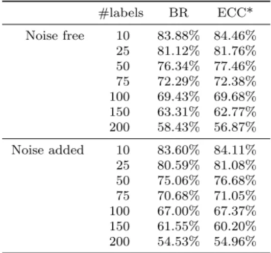
Table 3 AverageFmi

1 scores in test sets for datasets gener-ated explicitly withconditional dependency, see Section 6.2

#labels BR ECC* Noise free 10 83.88% 84.46% 25 81.12% 81.76% 50 76.34% 77.46% 75 72.29% 72.38% 100 69.43% 69.68% 150 63.31% 62.77% 200 58.43% 56.87% Noise added 10 83.60% 84.11% 25 80.59% 81.08% 50 75.06% 76.68% 75 70.68% 71.05% 100 67.00% 67.37% 150 61.55% 60.20% 200 54.53% 54.96%

Table 4 Significant differences for several number of labels using a Wilcoxon two-sided signed rank test. Thep-values in significant differences (or) were always below 0.01. For those cases in which the difference was not significant (=),∼ the obtainedp-value was greater than 0.60

Noise Range of Labels Significant Free {10,25,50} ECC*BR

{75,100} ECC*∼= BR

{150,200} ECC*BR Added {10,25,50,75} ECC*BR

{100,150,200} ECC*∼= BR

labels belongs to{10,25,50,75,100,150,200}, and the label dependence is in [0.1..0.35], measured using (11). The base learner for both methods was SVM (Chang and Lin, 2011) with a Gaussian kernel (RBF). The pa-rameters C and γ (for the Gaussian kernel) were ad-justed with a grid search using the validation dataset generated. The parameters could vary in C ∈ {10i _:

i = −1, . . . ,3}, γ ∈ {10−3_,10−2_,10−1_{,0.3,0.5,1}. For} ECC we used the implementation by Dembczy´nski et al (2010), denoted as ECC*. This means that, unlike Read et al (2011b), we did not apply any threshold selection method for deciding the relevance of a label. Of course the same policy was applied for BR. The number of CC models in a ECC* classifier was set to 10.

To compare the performance of BR and ECC* on this collection, we used the micro-averageF1scores (4). We selectedF₁mi for several reasons. On the one hand, we did not employ Hamming loss or macro-average mea-sures because BR optimizes such meamea-sures when a proper base learner is used. On the other hand, ECC* does not optimize any particular measure, mainly because it is an ensemble method. Thus, we selected a inter-mediate measure in which ECC* seems to outperform

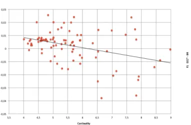
Figure 1 Dataset Cardinality. In the X-axis is the cardinal-ity, while in Y-axis the difference in terms of Fmi

1 between ECC* and BR. Each point represents the results for a dataset and when it is above 0 indicates that ECC* outperforms BR

BR, according to previous studies cited at the beginning of this section, with, basically, the same experimental setup. Also, ECC* is among the best methods in terms ofF₁miin the results reported by Madjarov et al (2012), performing better than BR.

7.2 Experimental results

Table 3 shows the average scores achieved by BR and ECC*. Additionally, Table 4 summarizes the significant differences between both learners using a Wilcoxon two-sided signed rank test.

The first evidence is that ECC* is significantly bet-ter than BR with a low number of labels, both for noise free and noisy datasets. These results are quite coherent with those reported by Read et al (2011b). In that paper, the experimental results were made with 15 datasets; only two of them have more than 103 labels.

Nevertheless, the differences between the two meth-ods become smaller when the number of labels increases; even BR significantly outperforms ECC* for noise free datasets and more than 100 labels. Maybe the reason is the accumulation of errors forced by the Classifier Chains algorithm of ECC*, which is more likely to hap-pen when the number of labels is large. This result could not be obtained using only benchmark datasets, simply because there are not enough datasets to statistically support this conclusion.

Our experiments, based on synthetic datasets, al-low us to analyze more aspects. For instance, Figure 1 depicts the performance of both methods with respect to the cardinality. Each point shows the results for a dataset in which X-axis represents the cardinality and

Figure 2 Dataset Label Dependency. In the X-axis is the label dependence, while in Y-axis is the difference in terms of Fmi

1 between ECC* and BR. Each point represents the results for a dataset and when its above 0 indicates that ECC* outperforms BR

Y-axis the difference in terms of Fmi

1 between ECC* and BR. Thus, a point above 0 in the Y-axis indi-cates that ECC* outperforms BR in that dataset. The graphic demonstrates that for those datasets with lower cardinality ECC* is much better, but when the cardi-nality is higher the result is just the opposite, BR ame-liorates the scores of ECC*.

But the most interesting analysis is perhaps that which studies the performance in function of label de-pendency, see Figure 2. This graphic is equivalent to the previous one: Y-axis represents again the difference in terms ofFmi

1 between ECC* and BR, but now the X-axis stands for the label dependency of the datasets measured applying (11). Despite the results seem quite mixed, the tendency line shows again that the scores of ECC* tend to be worse in comparison with those of BR when the label dependency increases. With a low label dependency, ECC* is clearly better, but for larger values BR is able to be at least competitive, and some-times superior.

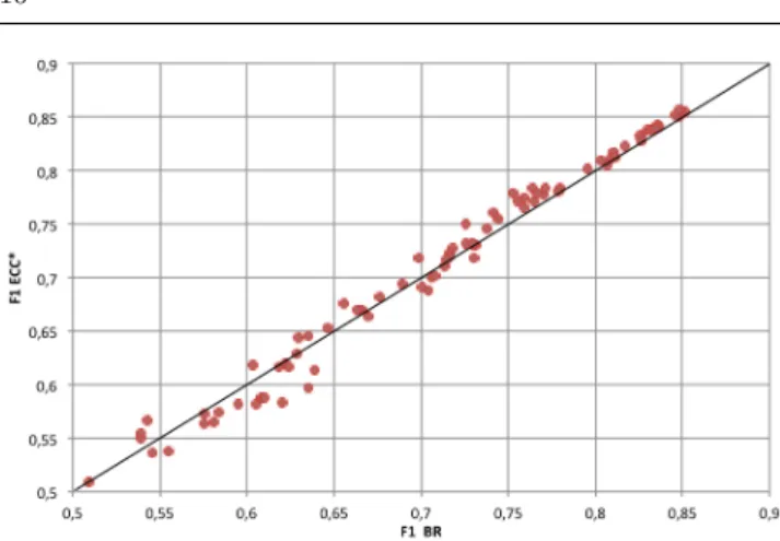
Finally, the scores of each of the 84 datasets are also reported graphically in Figure 3. The goal is to repre-sent somehow the complexity of the datasets, measured in terms ofF1mi: the greater theF1mivalue the easier the learning task. In this case, the meaning of the axises is different. Each point represents the results for a dataset, but now X-axis is theF₁miscore for BR, and Y-axis the

Fmi

1 result for ECC*. Therefore, those points above the diagonal correspond to datasets in which ECC* outper-forms BR, and the other way around. When the tasks are easier, with higherFmi

1 results, ECC* is better, but when theFmi

1 scores decrease, then BR usually achieves the best results.

Figure 3 Dataset Complexity. Each point is a pair of F1mi scores achieved in the same dataset by BR and ECC*. Points above the diagonal represent datasets where ECC* outper-forms BR

Actually, all these analyses reflect the same conclu-sion: when the learning task is easier (less cardinality or less label dependency or a fewer number of labels), ECC* performs better. But when the domain is more complex, with more labels or a greater cardinality or label dependency, then BR is at least competitive and sometimes superior.

The purpose of these experiments is not just to an-alyze BR and ECC* from another perspectives. The goal was also to point out that it is difficult to ex-tract useful conclusions, statistically supported, using only benchmark datasets; there are too few domains given the complexity of ML classification. Being this the case, synthetic datasets may allow us to gain more insight about the behavior of ML methods, analyzed them with respect to different factors as we have shown with this study.

8 Conclusions

In this article we tried to demystify some clich´es about ML classification and its main baseline method, Binary Relevance. For instance, one interesting point is to ac-knowledge the properties of BR, not only its compu-tational complexity, but also that it is well-tailored to produce good ML classifiers for several ML loss func-tions. Hamming loss and macro-averages are clearly ori-ented to the use of learners that consider each label separately. A correct implementation of BR, using the appropriate base learner for the target loss function, should be enough if one wants to achieve good scores. Thus the main efforts of ML community should be fo-cused on devised methods for optimizing other kind of measures.

New proposals can obviously improve the perfor-mance of BR for other perforperfor-mance metrics. However, the experimental studies are limited due to the lack of benchmark domains. There are just a few publicly avail-able domains and they cover a small and biased pro-portion of the huge possibilities of ML datasets. Under these circumstances, our proposal is to combine bench-mark with synthetic datasets to perform more complete experimental studies. In this paper we have used a ML dataset generator that produces synthetic domains in which the user can select properties like the number of labels, the cardinality and the label dependency.

We have compared the efficacy of BR and an Ensem-ble of Classifier Chains using a collection of synthetic problems. The main conclusion is that the performance of ECC* dramatically drops when the complexity of the dataset increases —a larger number of labels or a greater cardinality or a higher label dependency— while BR is quite competitive under these circumstances. This is only an example of a situation that current experi-mental settings based on the benchmark datasets avail-able are not avail-able to detect.

Acknowledgements The research reported here is supported in part under grant TIN2011-23558 from the Ministerio de Econom´ıa y Competitividad, Spain. We would also like to ac-knowledge all those people who generously shared the datasets and software used in this paper.

References

Bielza C, Li G, Larra˜naga P (2011) Multi-dimensional classification with bayesian networks. International Journal of Approximate Reasoning 52(6):705–727 Chang CC, Lin CJ (2011) LIBSVM: A library for

sup-port vector machines. ACM Transactions on Intel-ligent Systems and Technology 2:27:1–27:27, soft-ware available at http://www.csie.ntu.edu.tw/ ~cjlin/libsvm

Cheng W, H¨ullermeier E (2009) Combining Instance-Based Learning and Logistic Regression for Multil-abel Classification. Machine Learning 76(2):211–225 Dembczy´nski K, Cheng W, H¨ullermeier E (2010) Bayes optimal multilabel classification via probabilis-tic classifier chains. Proceedings of the 27th Interna-tional Conference on Machine Learning (ICML) pp 279—286

Dembczy´nski K, Waegeman W, Cheng W, H¨ullermeier E (2011) An exact algorithm for f-measure maximiza-tion. In: Proceedings of the Neural Information Pro-cessing Systems (NIPS), pp 1404–1412

Elisseeff A, Weston J (2001) A kernel method for multi-labelled classification. In: In Advances in Neural

In-formation Processing Systems 14, MIT Press, pp 681–687

Godbole S, Sarawagi S (2004) Discriminative methods for multi-labeled classification. In: Lecture Notes in Artificial Intelligence (Subseries of Lecture Notes in Computer Science), vol 3056, pp 22–30

Joachims T (2005) A support vector method for multi-variate performance measures. In: Proceedings of the ICML ’05, pp 377–384

Lastra G, Luaces O, Quevedo J, Bahamonde A (2011) Graphical feature selection for multilabel classifica-tion tasks. In: Gama J, Bradley E, Hollm´en J (eds) Proceedings of Advances in Intelligent Data Analysis X (IDA 2011), Springer, Lecture Notes in Computer Science, vol 7014, pp 246–257

Madjarov G, Kocev D, Gjorgjevikj D, Deroski S (2012) An extensive experimental comparison of meth-ods for multi-label learning. Pattern Recognition 45(9):3084–3104

Monta˜n´es E, Quevedo J, del Coz J (2011) Aggregating independent and dependent models to learn multi-label classifiers. Proceedings of the European Confer-ence on Machine Learning and Knowledge Discovery in Databases (ECLM-PKDD) pp 484–500

Petterson J, Caetano T (2010) Reverse multi-label learning. Advances in Neural Information Processing Systems 23:1912—1920

Quevedo JR, Luaces O, Bahamonde A (2012) Multil-abel classifiers with a probabilistic thresholding strat-egy. Pattern Recognition 45(2):876–883

Read J, Pfahringer B, Holmes G (2009a) Gen-erating Synthetic Multi-label Data Streams. In: ECML/PKKD 2009 Workshop on Learning from Multi-label Data (MLD’09), pp 69–84

Read J, Pfahringer B, Holmes G, Frank E (2009b) Clas-sifier Chains for Multi-label Classification. In: Pro-ceedings of European Conference on Machine Learn-ing and Knowledge Discovery in Databases (ECML-PKDD), pp 254–269

Read J, Bifet A, Holmes G, Pfahringer B (2011a) Streaming multi-label classification. JMLR Work-shop and Conference Proceedings (Second WorkWork-shop on Applications of Pattern Analysis) 17:19–25 Read J, Pfahringer B, Holmes G, Frank E (2011b)

Clas-sifier chains for multi-label classification. Machine Learning 85(3):333–359

Schapire R, Singer Y (2000) Boostexter: A boosting-based system for text categorization. Machine learn-ing 39(2):135–168

Tsoumakas G, Katakis I (2007) Multi Label Classifi-cation: An Overview. International Journal of Data Warehousing and Mining 3(3):1–13

Tsoumakas G, Katakis I, Vlahavas I (2010a) Mining Multilabel Data. Data Mining and Knowledge Dis-covery Handbook pp 667–685

Tsoumakas G, Katakis I, Vlahavas I (2010b) Random k-Labelsets for Multi-Label Classification. IEEE Trans-actions on Knowledge Discovery and Data Engineer-ing 23(7):1079–1089

Zaragoza J, Sucar L, Bielza C, Larra˜naga P (2011) Bayesian chain classifiers for multidimensional classi-fication. In: Twenty-Second International Joint Con-ference on Artificial Intelligence (IJCAI), pp 2192– 2197

Zhang ML, Zhou Z (2007) ML-KNN: A Lazy Learning Approach to Multi-label Learning. Pattern Recogni-tion 40(7):2038–2048