Essays on Correlation Modelling

(1)

Mads Stenbo Nielsen

The PhD School of Economics and Management

PhD Series 31.2011

Essays on Corr

elation Modelling

copenhagen business school handelshøjskolen solbjerg plads 3 dk-2000 frederiksberg danmark www.cbs.dk ISSN 0906-6934 Print ISBN: 978-87-92842-22-0 Online ISBN: 978-87-92842-23-7

(2)

Essays on Correlation Modelling

Mads Stenbo Nielsen

Ph.D. thesis

Department of Finance Copenhagen Business School August 2011

(3)

Mads Stenbo Nielsen

Essays on Correlation Modelling

1st edition 2011 PhD Series 31.2011 © The Author ISSN 0906-6934 Print ISBN: 978-87-92842-22-0 Online ISBN: 978-87-92842-23-7

“The Doctoral School of Economics and Management is an active national and international research environment at CBS for research degree students who deal with economics and management at business, industry and country level in a theoretical and empirical manner”.

No parts of this book may be reproduced or transmitted in any form or by any means, electronic or mechanical, including photocopying, recording, or by any information storage or retrieval system, without permission in writing from the publisher.

(4)

Preface

This thesis is the result of my Ph.D. studies at the Department of Finance, Copenhagen Business School. The thesis consists of three essays that cover diﬀerent aspects of correlation modelling in corporate default risk. Each essay is self-contained and can be read independently.

Structure of the thesis

The common theme across all three essays is the role of correlation in corporate default risk. While the likelihood for a given firm to default depends on a number of firm-specific characteristics such as earnings, debt outstanding, cash holdings, total assets, stock returns etc., there are also cross-sectional comovements in default probabilities that cannot be explained by idiosyncratic factors. E.g. the general state of the economy, sector-wide up- or downswings, and the financial soundness of competitors and business partners may all contribute to a clustering of default risk over time.

Accounting for such correlation is important for both pricing and risk management of portfolios of defaultable assets, and the thesis addresses diﬀerent ways to capture correlation both in actual default probabilities as well as in prices of defaultable assets and credit derivatives. The common goal of the thesis is to formulate and estimate quantitative models of default risk with speciﬁc attention to the importance of default correlation, and use that to gain further understanding of the nature of correlation in default risk.

In the ﬁrst essay (co-authored with David Lando, Copenhagen Business School), we investigate statistical techniques for testing the adequacy of “conditional independence”– based intensity models of default. Previous literature has used a time-change technique

to analyze these models and jointly test the intensity speciﬁcationandthe “conditional

(7)

Preface

U.S. industrial firms, we show that the time-change technique is, however, mainly a test of the intensity specification. We further demonstrate by a simple example how a violation of the conditional independence assumption may not be captured by the time-change test, and we give the intuition behind this result. We conclude by proposing alternative tests that explicitly account for the impact of previous defaults on the default intensity, but we find little evidence of this type of correlation in our empirical sample.

The second essay (co-authored with Peter Feldhütter, London Business School) addresses the pricing of correlation in CDO tranche spreads, which are essentially call option spreads on default correlation among a portfolio of defaultable entities. We provide an intensity-based model that allows us to split the default risk into a systematic (correlation) and an idiosyncratic component, and we show how to estimate the model without imposing the restrictive parameter constraints appearing in previous literature. We ﬁnd that the systematic default component is an explosive process with low volatility, whereas the idiosyncratic default risk is more volatile but less explosive. We further ﬁnd that the model is able to capture both the level and time series dynamics of CDO tranche spreads.

The third and ﬁnal essay concerns time series variation in corporate bond spreads induced by variation in the state of the economy. The essay documents how the level and slope of empirical credit spread curves vary with the business cycle, and it develops a structural credit risk model with jump risk that allows for explicit dependence on the state

of the economy. The model uniﬁes several existing models that focus entirely oneither

jumporbusiness cycle risk. Subsequent estimation of the model reveals the importance

of accounting for both jump and business cycle risk in order to capture the time-variation in empirical credit spread curves. In addition, the model gives predictions for net beneﬁts to debt and optimal capital structure that are in line with existing literature.

English and Danish summary of each essay is provided below.

Publication details

The ﬁrst essay is an extended version of a paper published in theJournal of Financial

Intermediation, volume 19, page 355–372, and the second essay has been accepted for

(8)

Acknowledgements

The essays in this thesis have beneﬁtted greatly from comments and suggestions from a number of people, and they are mentioned with each of the essays. However, a few people deserve a special mention.

First of all, I am deeply indebted to my advisor, professor David Lando, for his constant encouragement, commitment to, and belief in my work – even at times when little progress was made. His guidance has been an invaluable source of inspiration and his critical comments have affected much of the work presented in this thesis. I similarly wish to thank assistant professor Peter Feldhütter for sharing his previous work on CDO pricing with me, for his excellent co-authorship on the second essay, and not least for suggesting me to apply for a Ph.D. scholarship in the first place. Furthermore, I thank current and previous colleagues and fellow Ph.D. students at the Department of Finance, CBS, for many rewarding discussions as well as for many hours of great fun. In particular, I thank Claus Bajlum, Jens Dick-Nielsen, Peter Feldhütter, René Kallestrup, and Morten Nalholm for always taking the time to listen to my ideas and providing me with useful feedback, and a special thanks to Jens Dick-Nielsen for our many stimulating five-minute-seminars. Moreover, I am indebted to Derek Moore for always supplying instant and accurate IT assistance, and to Peter Raahauge for patiently introducing me to the world of Matlab. In addition, I wish to thank professor Kristian Miltersen and associate professor Christian Riis Flor for participating in my pre-defense and for providing me with a range of critical and useful comments.

Finally, I wish to thank my family and friends for always being there for me and for their unconditional support and belief in me, without which this thesis would not have been completed.

Mads Stenbo Nielsen Copenhagen, August 2011

(9)

(10)

Summary

This section contains English and Danish summaries of the three essays that comprise the thesis.

English summary

Essay I: Correlation in corporate defaults: Contagion or conditional independence?(co-authored with David Lando, CBS)

The ﬁrst essay studies statistical procedures for testing the validity of intensity-based

models ofactualdefaults. Such models are often applied under an additional assumption

of conditional independence, whereby the default event is assumed to be conditionally independent of the factors appearing in the speciﬁcation of the default intensity. Das,

Duﬃe, Kapadia, and Saita (2007) (DDKS) propose a statistical procedure tojointlytest

the speciﬁcation of the default intensity andthe conditional independence assumption

through time-changing observed defaults into independent Poisson-distributed variables. In an empirical application to U.S. default data, DDKS strongly reject the validity of the joint hypothesis of well-speciﬁed intensities and conditional independence.

This leaves open the question of whether their rejection is due to incorrectly specified intensities or a violation of the conditional independence assumption. Using an extensive data set covering 24 years and a total of 2,557 U.S. industrial firms, we show that the rejection is likely to be caused by misspecified default intensities. We first confirm the results obtained by DDKS using their intensity specification and subsequently show that by employing an extended specification, we can no longer reject the joint hypothesis of well-specified intensities and the conditional independence assumption. To strengthen our result, we add further Poisson test statistics to those appearing in DDKS, but this does

(11)

English summary

not change our conclusion.

We subsequently nuance our result by showing that the time-change procedure is, in fact, unable to capture certain violations of the conditional independence assumption. We set up a simple example to demonstrate how default contagion that spreads through the

variables in the default intensity speciﬁcation will notbe captured by the time-change

approach. We therefore need additional test procedures to account for the presence of contagion in corporate default data, and we propose to use both regression analysis as well as a Hawkes specification of the intensity. In the latter approach, previous defaults are allowed to directly impact the likelihood of default for firms that are still alive. We apply both types of tests to our empirical data and find only limited evidence of default contagion.

Essay II: Systematic and idiosyncratic default risk in synthetic credit markets(co-authored with Peter Feldhütter, LBS)

The second essay develops a ﬂexible intensity-based model for pricing correlation-dependent credit derivatives. The model features both idiosyncratic and systematic default risk and ensures consistent pricing of single- and multi-name credit derivatives. The key idea behind the model is to infer term structures of risk-neutral default probabilities from single-name Credit Default Swaps (CDSs), and use that to estimate the systematic default component of each ﬁrm’s default probability from tranche spreads of Collateralized Debt Obligations (CDOs).

The default intensity of each individual ﬁrm is assumed to be a sum of an idiosyncratic component and a suitable scaling of a systematic component. We show by a straightforward argument how the scaling of the systematic component may be inferred from a simple linear regression, and we demonstrate in our empirical application that this choice of weighting is consistent with the intuitive scaling of systematic default risk applied in previous literature.

Central to our approach is the fact that we can leave the idiosyncratic default component unmodelled, and thereby avoid the restrictive parameter contraints imposed in existing literature. Thus, we are able to specify a highly ﬂexible model, while retaining a tractable estimation procedure, where only relatively few parameters have to be estimated.

(12)

Furthermore, since our model only relies on liquid, synthetic credit derivatives (CDSs and CDOs), we are able to base our estimation of the model on a large data set of daily data. In our implementation we use 90,600 credit spreads covering a total of 120 days.

When estimating the model we ﬁnd that systematic default risk is explosive and has low volatility, whereas idiosyncratic risk on the other hand is less explosive but has larger volatility. Finally, we ﬁnd that the model is able to capture both the level and time series dynamics of the CDO tranche spreads in our sample.

Essay III: Credit spreads across the business cycle

The third essay takes a completely diﬀerent approach to the modelling of default risk correlation than the ﬁrst two. Instead of using default intensities, the third essay relies on a structural approach in order to describe business cycle variation in corporate credit spreads.

I first demonstrate how the level and slope of empirical credit spreads are negatively, respectively positively correlated with consumption growth, and I show that these patterns are persistent across both investment and speculative grade issuers. In particular, I document that the credit spread curve is generally upward-sloping in times of high economic growth, but becomes flat or even inverted as the economy approaches a trough. I further show that the variation in the slope of the credit spread curve may result from shifts in the relative distribution between short- and long-term risk. As economic growth declines, not only does the level of default risk increase, but also the relative importance of short-term default risk increases. As a proxy for short-term risk, I consider jumps in equity returns, and I find empirically that both positive and negative jumps covary with the business cycle, with larger jumps in times of low economic growth. I develop a new technique in order to estimate the jumps, and I show that the detected jumps are consistent with the common interpretation of jumps as representing the arrival of new information to the market.

To capture the observed business cycle correlation with both level and slope of corporate credit spread curves, I formulate a structural credit risk model that takes both jump and business cycle risk into account. This model is the ﬁrst to consider both risk factors in a joint framework, and it uniﬁes several existing models that focus entirely on

(13)

Dansk resumé

just one of these two factors.

I estimate the model on a firm-by-firm basis using daily data from 1962 to 2006, and the estimation shows that the model is able to replicate the observed variation in both level and slope of corporate credit spreads. In particular, the model-implied credit spread curves are upward-sloping when economic growth is high, and flat or downward-sloping when economic growth is low. The ability of the model to generate such curves hinges

crucially on theinterplaybetween jump and business cycle risk, with jump risk increasing

during economic downturns. Moreover, the estimated model yields predictions for net beneﬁts to debt and optimal capital structure that are in line with results in the existing literature.

Dansk resumé

Essay I: Korrelation blandt virksomheders fallithændelser: Smitte-eﬀekter eller betinget uafhængighed? (medforfatter David Lando, CBS)

Det første essay undersøger statistiske metoder til at teste brugbarheden af

intensitets-baserede modeller for observerede fallithændelser. Sådanne modeller anvendes ofte

i sammenhæng med en yderligere antagelse om betinget uafhængighed, hvorved fallithændelsen antages at være betinget uafhængig af de faktorer, der indgår i speciﬁkationen af fallitintensiteten. Das, Duﬃe, Kapadia, and Saita (2007) (DDKS)

foreslår en statistisk metode til på samme tid at teste både speciﬁkationen af

fallitintensiteten og antagelsen om betinget uafhængighed ved at tidstransformere

observerede fallithændelser til uafhængige Poisson-fordelte variable. I et empirisk studie af amerikanske fallitdata forkaster DDKS entydigt gyldigheden af den dobbelte hypotese om korrekt speciﬁcerede intensiteter og betinget uafhængighed.

Det rejser spørgsmålet om, hvorvidt deres resultat skyldes forkert specificerede intensiteter eller et fravær af betinget uafhængighed. På baggrund af data for i alt 2.557 amerikanske industrivirksomheder over en 24-årig periode viser vi, at resultatet formentlig skyldes fejlagtigt specificerede intensiteter. Vi replikerer først DDKS’ resultat ved at bruge deres foreslåede intensitetsspecifikation, og vi viser derefter at ved at bruge en udvidet specifikation, er det ikke længere muligt at forkaste den dobbelte hypotese om korrekt specificerede intensiteter og betinget uafhængighed. For at underbygge vores resultat

(14)

tilføjer vi yderligere Poisson-teststørrelser til dem, der allerede optræder i DDKS, men det ændrer ikke på vores konklusion.

Vi nuancerer herefter vores konklusion ved at vise, at tidstransformationsmetoden ikke er i stand til at opfange bestemte overtrædelser af antagelsen om betinget uafhængighed. Vi opstiller et simpelt eksempel, der viser hvorledes smitte-eﬀekter,

der optræder via variablene i speciﬁkationen af fallitintensiteten, ikke fanges af

tidstransformationsmetoden. Det er derfor nødvendigt med yderligere tests for at kunne opdage smitte-effekter blandt virksomheders fallithændelser. Vi foreslår i den forbindelse at benytte såvel regressionsmetoder som en Hawkes-specifikation af fallitintensiteten. Sidstnævnte tillader at forudgående fallithændelser kan have en direkte effekt på sandsynligheden for fallit blandt de tilbageværende virksomheder. Vi anvender begge typer af testprocedurer på vores empiriske data, og finder kun begrænsede tegn på eksistens af smitte-effekter.

Essay II: Systematisk og idiosynkratisk fallitrisiko i “syntetiske” kreditrisiko-instrumenter(medforfatter Peter Feldhütter, LBS)

Det andet essay opstiller en ﬂeksibel intensitetsbaseret model til prisfastsættelse af korrelationsafhængige kreditrisiko-instrumenter. Modellen omfatter både idiosynkratisk og systematisk fallitrisiko og sikrer en konsistent prisfastsættelse af aﬂedte instrumenter, der involverer både én enkelt såvel som en hel gruppe af virksomheder. Den grund-læggende idé bag modellen er at udlede kurver af risiko-neutrale fallitsandsynligheder på baggrund af handlede Credit Default Swaps (CDS’er), og bruge disse til at estimere den systematiske del af hver enkelt virksomheds fallitsandsynlighed ved hjælp af Collateralized Debt Obligation (CDO) tranche-spænd.

Hver enkelt virksomheds fallitintensitet antages at være en sum af en idiosynkratisk faktor og en passende skalering af en systematisk faktor. Vi viser med et simpelt argument, hvorledes skaleringen af den systematiske faktor kan udledes fra en almindelig lineær regression, og viser siden hen i den empiriske del af papiret, hvorledes resultatet af denne skalering stemmer overens med den ad hoc skalering af systematisk fallitrisiko, som tidligere studier har anvendt.

(15)

Dansk resumé

del af fallitrisikoen, og at vi derved undgår de strenge parameterrestriktioner, der optræder i den eksisterende litteratur. Vi er således i stand til at speciﬁcere en yderst ﬂeksibel model, der samtidig er overkommelig at estimere, idet det samlede antal parametre, der skal estimeres, er forholdsvis begrænset. Eftersom modellen alene bygger på likvide, “syntetiske” kreditrisiko-instrumenter (CDS’er og CDO’er), er det muligt at basere estimation af modellen på en stor mængde af daglige data. I vores implementering af modellen bruger vi 90.600 kreditspænd fordelt over en periode på i alt 120 dage.

Vores estimation af modellen viser, at den systematiske kreditrisiko er “eksplosiv” omend med lav volatilitet, mens den idiosynkratiske risiko er mindre eksplosiv men mere volatil. Endelig viser estimationen, at modellen er i stand til at fange både niveauet og tidsserievariationen i de empiriske CDO tranche-spænd.

Essay III: Konjunkturvariation i virksomheders kreditspænd

Det tredje essay benytter en helt anden tilgang til modellering af korrelation i virksomheders kreditrisiko end de to første essays. I stedet for at basere sig på fallitintensiteter anvendes i stedet en strukturel model til at beskrive konjunkturvariationen i virksomheders kreditspænd.

Indledningsvis viser jeg, hvorledes niveauet og hældningen på empiriske kreditspænds-kurver er henholdvis negativt og positivt korreleret med væksten i privatforbruget. Mere speciﬁkt så viser jeg, at kreditspændskurver generelt har positiv hældning i perioder med høj økonomisk vækst, mens de ﬂader ud og i visse tilfælde ligefrem inverterer i perioder med lav vækst.

Jeg demonstrerer dernæst, at konjunkturvariationen i kurvernes hældning kan knyttes til ændringer i den relative fordeling mellem kort- og langsigtet kreditrisiko. I takt med at den økonomiske vækst aftager, stiger både det absolutte niveau af kreditrisiko såvel som den relative betydning af kortsigtet kreditrisiko. Som mål for kortsigtet kreditrisiko anvender jeg spring i realiserede aktieafkast, og jeg bruger det til at dokumentere konjunkturfølsomhed i størrelsen af både positive og negative aktiespring, hvor springene generelt er større i perioder med lav økonomisk vækst. Til brug for estimation af aktiespringene udvikler jeg en ny metode, som jeg påviser er i overensstemmelse med den traditionelle fortolkning af aktiespring som udtryk for tilgang af ny information til

(16)

aktiemarkedet.

Til beskrivelse af den dokumenterede korrelation mellem samfundsøkonomiske konjunkturer og henholdsvis niveau og hældning på virksomheders kreditspændskurver opstiller jeg herefter en strukturel kreditrisikomodel, der tager højde for både spring-og konjunkturrisici. Dette er den første strukturelle model, som tager hensyn til begge risikofaktorer på samme tid. Som specialtilfælde indeholder den adskillige eksisterende modeller, der alene fokuserer på den ene af de to faktorer.

Jeg estimerer modellen for en række virksomheder på baggrund af daglige data for perioden fra 1962 til 2006, og estimationen viser at modellen er i stand til at replikere den observerede variation i både niveau og hældning på virksomheders kreditspændskurver. Specielt så har modellens kurver positiv hældning, når den økonomiske vækst er høj, mens kurverne er ﬂade eller har negativ hældning, når væksten er lav. Modellens evne til

at generere disse kurver er tæt knyttet tilsamspilletmellem spring- og konjunkturrisici,

der medfører en forøget springrisiko i perioder med lav økonomisk vækst. Den estimerede model giver desuden anledning til forudsigelser vedrørende nettofordelen ved udstedelse af gæld samt valget af optimal kapitalstruktur. For begge dele gælder, at disse forudsigelser er i overensstemmelse med resultater i den eksisterende litteratur.

(17)

(18)

Introduction

When a firm borrows money to finance its activities, it pays an interest which, among other things, is influenced by the firm’s ability to service its loan. When the lender, say, a bank, has to determine the appropriate interest rate to charge, it therefore has to assess the likelihood that the firm will default on its obligation. If the bank has also granted loans to other firms, it likewise has to assess the likelihood of default for each of these firms. Hence, it is necessary for the bank to have models that it can use to estimate the probability of default for each of its borrowers.

There is strong empirical evidence that defaults cluster over time, simply because in times of low economic growth more firms struggle to repay their existing loans and/or experience increasing difficulties in obtaining new loans. As a result, the bank is likely to suffer excessive losses in such periods, and it is therefore not enough just to estimate the probability of default for each individual borrower. It is equally important to also take

into account thecorrelationbetween defaults in order to capture the clustering of defaults

(and hence losses) over time.

If we consider a speciﬁc borrower and letτdenote his (stochastic) default time, then the

object of interest is the probability distribution ofτ. Default risk models are traditionally

classiﬁed as eitherintensitymodels orstructuralmodels, depending on the way they model

the distribution ofτ. For intensity models, the distribution ofτ is described in terms of

its defaultintensity

lim

dt→0

P(t < τ≤t+dt|τ > t)

dt =λt

that determines the probability of instant default at any time t. Intensity models make

no a priori assumptions about the behaviour of λt and thus provide a highly ﬂexible

framework, which is used both for default probability modelling as well as for pricing of credit risky securities. The deﬁnition of the default intensity implies that the distribution

(19)

Introduction

ofτ has the equivalent representation

P(τ > t) = exp

− t

0 λsds

which shows that the mathematical structure of intensity models is closely related to models of default-free interest rates. This has the obvious advantage that many of the techniques used to model ﬁxed income instruments can also be used to model default risk as pointed out e.g. in Lando (1998) and Duﬃe and Singleton (1999).

Intensity models find their strength in the flexible specification of the default intensity, whereas structural models take a completely different approach. Here, the idea is to set up

speciﬁc economicstructuresbased on underlying factors that are believed to be the drivers

of default risk. Hence, structural models are significantly more restrictive in terms of their modelling flexibility, but offer instead important insights into the economic mechanisms

behind the distribution of the default timeτ. The ﬁrst papers along these lines were the

seminal works of Black and Scholes (1973) and Merton (1973; 1974) for which the latter two authors were awarded the Alfred Nobel Prize in Economic Sciences in 1997.

This thesis contains new results related to both of the classical ﬁelds of default risk models. Essay I and II contain empirical applications of intensity-based models to

estimation ofactualdefault probabilities and pricing of credit derivatives, respectively,

and Essay III develops a new structural credit risk model. The common theme across all three essays is the role of correlation between default times for a pool of borrowers, and how to model and estimate this correlation from observed defaults and from prices of traded securities.

The first essay, Essay I (co-authored with David Lando, CBS), studies various specifications of intensity-based models and discuss their ability to match the probability of default in a large sample of U.S. industrial firms. The paper builds on earlier work by Duffie, Saita, and Wang (2007) and Das, Duffie, Kapadia, and Saita (2007) on estimation and test of intensity models under an assumption of conditional independence between default events and default intensities. In this setting default correlation only enters through cross-correlation among the firm-specific and macroeconomic variables appearing in the specification of the default intensities. Das, Duffie, Kapadia, and Saita (2007) suggest a statistical procedure for testing this particular class of models, and in an empirical application the authors find that their proposed test rejects their conditional

(20)

independence intensity speciﬁcation.

The first contribution of Essay I is to show that a more careful specification of the default intensities, still working under the conditional independence assumption, changes the conclusion of Das, Duffie, Kapadia, and Saita (2007). Hence, it is no longer possible to reject the validity of intensity models specified using conditional independence. The second contribution of Essay I is then to demonstrate that the proposed test procedure is, in fact, insufficient to test the conditional independence assumption, since the assumption may be violated without the test procedure being able to detect this.

The third and ﬁnal contribution of Essay I is to propose and apply alternative tests using regression analysis and Hawkes processes (Hawkes 1971a;b). The latter type of process has a long-standing history e.g. in studies of earthquakes (see for example Ogata, Akaike, and Katsura (1982)), but has only recently gained attention in ﬁnancial applications (see for example Errais, Giesecke, and Goldberg (2010) and Shek (2010)).

In recent work related to Essay I, Duffie, Eckner, Horel, and Saita (2009) find that instead of changing the set of observable variables entering the default intensity, it is also possible to obtain an improved fit to empirical default data by incorporating latent variables. Unfortunately this approach also implies a significant increase in the statistical estimation uncertainty, and it does not provide any economic interpretation of the added latent factors.

Essay II (co-authored with Peter Feldhütter, LBS) also applies an intensity-based model to describe default risk and default correlation among a pool of borrowers. However, in contrast to Essay I default probabilities are not based on observations of actual defaults but instead inferred from prices of credit derivatives. The default correlation structure is again based on a conditional independence assumption and is thus similar to that of Essay I, except that now both idiosyncratic and systematic default risk are modelled as latent factors as opposed to observable factors in Essay I.

Although Essay II concerns the estimation of default risk, the estimation methodology draws heavily on techniques from the literature on default-free term structure modelling. Specifically, to infer term structures of default probabilities from prices of Credit Default Swap (CDS) contracts, we use an approach similar to the derivation of yield curves from observed bond prices suggested by Nelson and Siegel (1987). Similarly, for the parametrization of our systematic default component we use an affine jump-diffusion

(21)

Introduction

process in analogy with the extensive literature on aﬃne term structure models (see e.g. Duﬃe and Kan (1996), Dai and Singleton (2000), Collin-Dufresne, Goldstein, and Jones (2008)).

The first contribution of Essay II is that we exploit the whole term structure of CDS spreads to infer a corresponding term structure of default probabilities for each firm in our sample. This allows us in a novel way to remove the restrictive parameter contraints enforced in earlier work by Duffie and Gârleanu (2001) and Mortensen (2006). Moreover, our approach enables us to split the total amount of default risk into an idiosyncratic and a systematic part. This potentially allows for more detailed analyses of the forces driving market-implied default risk compared e.g. to the papers of Longstaff and Rajan (2008) and Errais, Giesecke, and Goldberg (2010), where only the aggregate default risk is considered.

In the second contribution of the paper, we give a theoretical argument for how to estimate the weight on the systematic default component in each ﬁrm’s default intensity. We further demonstrate that the resulting empirical estimates are similar to those implied by the ad hoc method applied in previous literature. Our third and ﬁnal contribution

is to estimate our model on a large empirical data set and thereby show that it is

possible to formulate a default correlation model that can match the level and time series

dynamics of both single-name CDS spreadsandcorrelation-dependent, multi-name CDO

(Collateralized Debt Obligation) spreads at the same time.

The scope of Essay II is to capture the correlation implied by observed market prices of credit risky securities, and not to determine the fundamental economic sources of default correlation. This is instead the focal point of Essay III. Here, I apply the idea that correlation (in actual defaults as well as in prices of credit risky securities) is to some extent caused by common variation in macroeconomic variables. This is already exploited in the intensity-model considered in Essay I, and in Essay III it is used to develop a structural credit risk model with the purpose of explaining business cycle variation in corporate credit spreads.

The basic setting of the model follows the structural framework introduced in Leland (1994b), where a ﬁrm’s debt and equity are viewed as claims to underlying assets, and the

default time τ is the ﬁrst time asset value falls below some prespeciﬁed threshold. The

(22)

diﬀerent directions:eitherto allow for jumps in asset value (Hilberink and Rogers (2002),

Cremers, Driessen, and Maenhout (2008), Chen and Kou (2009))orto take business cycle

ﬂuctuations in asset value into account (Hackbarth, Miao, and Morellec (2006), Bhamra, Kuehn, and Strebulaev (2010a;b), Chen (2010)).

The ﬁrst contribution of Essay III is to document how both level and slope of observed credit spreads vary with the state of the economy, and to link this to similar ﬂuctuations

in empirical jump behaviour. This suggests that both jumpsandbusiness cycle variation

have a role to play in explaining corporate credit spreads, and in the second contribution

of the paper I therefore construct a structural credit risk model that incorporatesbothrisk

factors at the same time. This essentially uniﬁes most of the models mentioned above, and I demonstrate that despite signiﬁcant additional model complexity, that arises when both jump and business cycle risk are included, it is still possible to obtain closed-form expressions for the market values of debt and equity.

The last two contributions of Essay III regard empirical aspects of the formulated structural model. While there already exists a comprehensive literature on jump parameter estimation using high-frequency data (see e.g. Barndorff-Nielsen and Shephard (2004; 2006), Huang and Tauchen (2005), Andersen, Bollerslev, Diebold, and Vega (2007)), it is not possible to apply these techniques to the estimation of my model, since reliable estimation of the business cycle related parameters requires a sample period of multiple decades over which high-frequency data is not available. Instead, I present an alternative method for estimation of the jump parameters, and I verify that the outcome of this alternative procedure is consistent with the common perception of jumps as representing arrival of new information to the market (see e.g. Maheu and McCurdy (2004), Lee and Mykland (2008)). In the last contribution of the paper, I perform a full firm-by-firm estimation of the model and I show that the resulting model-implied credit spread curves replicate the previously observed business cycle variation in empirical credit spreads.

Brieﬂy summing up, the overall purpose of this thesis is to gain further understanding of the importance of and mechanisms behind corporate default correlation, and the three essays in the thesis describe diﬀerent aspects of this correlation. Essay I looks at correlation in actual default probabilities, Essay II discusses correlation inmarket-implied default probabilities derived from prices of correlation-dependent credit derivatives, and Essay

(23)

Introduction

loss rates with particular focus on the underlying economic mechanisms driving these ﬂuctuations.

(24)

Essay I

Correlation in corporate defaults: Contagion or

conditional independence?

∗

Co-authored with David Lando, Copenhagen Business School.

Published in theJournal of Financial Intermediation (2010).†

∗_{The authors would like to thank Antje Berndt, Wolfgang Bühler, Richard Cantor, Michael Chernov,} Darrell Duﬃe, Kristian Miltersen, Tue Tjur, seminar participants at Mannheim University, University of Lausanne, University of Amsterdam, Moody’s, the Danish Doctoral School of Finance, the Nordic Finance Network, the Basel Conference on Risk Transfer Mechanisms and Financial Stability, the American Finance Association 2010 Meeting, the editor (George Pennacchi), and two anonymous referees for helpful comments. David Lando acknowledges support from the Danish Council for Independent Research. †_{The thesis version of the paper contains some additional results in section I.4.}

(25)

Correlation in corporate defaults: Contagion or conditional independence?

Abstract

We revisit a method used by Das, Duffie, Kapadia, and Saita (2007) (DDKS) to test the doubly stochastic assumption in intensity models of default. We show that using a different specification of the default intensity, and using the same test as DDKS, we cannot reject using an almost identical set of default histories recorded by Moody’s in the period from 1982 to 2006. We propose additions to the procedure as well as a Hawkes process alternative to test for violations of conditional independence but cannot detect contagion. We then observe that the test proposed by DDKS is mainly a misspecification test in that it will not detect contagion effects as long as individual firms have default intensities and there are no simultaneous jumps to default. Specifically, contagion spread through the explanatory variables (“covariates”) that determine the default intensities of individual firms will not be detected. We therefore perform different tests to see if firm-specific variables are affected by occurrences of defaults. Regression tests show that there is no influence from defaults on quick ratios, but some influence on distance-to-default.

(26)

I.1 Introduction

Can we think of time variation in the frequency of corporate defaults as controlled by “exogenous” factors with no feedback from actual defaults to these factors? Or can we statistically document “contagion effects” by which one firm’s default increases the likelihood of other firms defaulting?

In a recent paper Das, Duffie, Kapadia, and Saita (2007) (DDKS) test whether default events in an intensity-based setting can reasonably be modelled as “doubly stochastic”, i.e. as dependent solely on “exogenous” factors. Their approach is to transform the time scale using the sum of the default intensities estimated for individual firms and then test whether defaults on this transformed time scale behave as a standard Poisson process. Based on a time series of U.S. corporate defaults, they strongly reject that defaults can be modelled as doubly stochastic. DDKS view this test as a joint test of the specification

of the default intensities of the individual ﬁrmsandthe doubly stochastic assumption. A

core message of our paper is that the time transformation test should be thought of mainly as a misspeciﬁcation test. We need – and propose – other tests to look for contagion eﬀects that violate the doubly stochastic assumption.

Our first contribution is to show that a different specification of the intensity will in fact make us unable to reject the tests performed by DDKS. That is, using our specification of the intensity there is no excess default clustering. As DDKS we use the sample of firms listed in Moody’s default database. To make sure that the different conclusion is not merely a consequence of deviations in the data, we show that specifying the explanatory variables as in DDKS, we reject the assumption of conditional independence but using our specification, we are not able to reject using a large variety of tests. In essence, our change in specification consists in replacing a measure of the short rate with a measure of steepness of the term structure, adding industrial production (a variable also examined in DDKS) and adding the following three firm-specific variables: quick ratio, short-to-long debt and the book value of assets. We will discuss this choice of the explanatory variables below.

The fact that we are unable to reject the tests performed in DDKS with our covariates could lead us to conclude, that there are no detectable contagion eﬀects in the data. This conclusion is premature, however. Our second contribution is to show that when contagion

(27)

I.1 Introduction

takes place through firm covariates (as opposed to contagion by “domino effects”), this will not be detected by the test procedure followed in DDKS (and in the first part of our paper). To state this in more economic terms, if default of one firm causes, say, the book value of assets of another firm to fall, and this increases the intensity of default of the other firm, then as long as the book asset value is an explanatory variable in our estimation of default intensities of firms, we will not detect this as a contagion effect using the test based on time transformation. To explain the intuition behind this insight, we set up the simplest structure rich enough to illustrate a contagion effect which occurs through explanatory variables, but which is not detected by the test.

Our final contribution is to analyze contagion effects, both direct and through explanatory variables, and using both likelihood tests based on Hawkes processes and regression analysis. Hawkes processes, or self-exciting processes, are a class of counting processes which allow intensities to depend on the timing of previous events. When we use firm-specific variables in the Cox regressions, the Hawkes specification does not add any explanatory power. If we only condition on macroeconomic variables and look for contagion by checking through a Hawkes specification whether downgrade intensities increase following a default, then we do detect a contagion effect. Since this effect may be due to rating agency behaviour, we also perform regression tests to check for contagion through the firm-specific variables distance-to-default and the quick ratio to be defined below. We find some support for this.

There is ample evidence that corporate defaults are correlated. For example, Lang and Stulz (1992) show that bankruptcy announcements significantly decrease the value of a portfolio of competitor stocks. Several empirical studies document a large time variation in default frequencies and link this variation to, among other variables, business cycle indicators. Examples of this include Nickell, Perraudin, and Varotto (2000), Shumway (2001), Duffie, Saita, and Wang (2007), and many others. Since such indicators simultaneously affect the default probabilities of many firms, their variation induces correlation between default events just as variation of common factors in asset return models induce correlation between returns.

We also have indirect evidence that defaults are correlated from market prices of traded securities. For example, Credit Default Swap premia have signiﬁcant common movements and prices of tranches of Collateralized Debt Obligations (CDOs) can only be reasonably

(28)

explained if one assumes a signiﬁcant amount of default correlation. Of course, market prices of these securities reﬂect not only the physical probabilities of defaults but also contain an adjustment for risk. Still, it is fair to assume that the price patterns we observe for CDO tranches can at least partially be attributed to correlated default risk.

How to best model the correlation effects is less clear. The most tractable way from an analytical standpoint is to work under a conditional independence assumption, in which a common factor structure induces covariation between the default times of different firms. Conditionally on the evolution of the common factors, defaults are independent. This formulation is also referred to as a doubly stochastic setting. This is a setting in which default dependence is captured by business cycle related variables. The conditional independence structure is analyzed among other places in Jarrow, Lando, and Yu (2005), and it is applied to CDO modelling for example in Duffie and Gârleanu (2001).

A more direct way of inducing dependence between default times is to assume that there is contagion, i.e. that the actual default event of one ﬁrm either directly triggers the

default of other ﬁrms or causes their default probabilities to increase.1Some examples of

contagion models include Davis and Lo (2001), Jarrow and Yu (2001), Azizpour and Giesecke (2008), and Azizpour, Giesecke, and Kim (2011). This type of contagion is clearly relevant when ﬁrms belong to the same corporate family, for example through parent-subsidiary relationships, see for example Emery and Cantor (2005). The question we address here is whether this type of contagion is present even for ﬁrms which do not belong to the same corporate family.

Note that our focus in this paper is not on “informational” contagion in prices on equity, corporate bonds or Credit Default Swap premia as studied for example by Collin-Dufresne, Goldstein, and Helwege (2003) and Jorion and Zhang (2009). Rather, we focus on methods for testing for conditional independence in actual defaults. Also, our focus is only on models based on observables. We do not estimate intensity models with frailty as done for example in Azizpour and Giesecke (2008), Duﬃe, Eckner, Horel, and Saita (2009), and Chava, Stefanescu, and Turnbull (2011).

Before looking at hard evidence, it is interesting to note that when looking through the default histories in Moody’s default database, it is almost impossible to locate any 1_{It is also conceivable that defaults could cause the default probabilities of competing ﬁrms to}_decrease_,

(29)

I.1 Introduction

examples where the brief description of what caused a firm to default mentions other firms outside the corporate family. The vast majority of cases list reasons such as too much leverage, failing sales in declining markets, and lawsuits – effects that are typically captured through either firm-specific explanatory variables or market-wide conditions. Indeed, looking at the points in time where the defaults seem to cluster more than what can be explained by the aggregate intensity in the DDKS specification, we find that none of the default stories contains any instances of contagion from other firms in the sample. This seems to rule out at least the direct domino effect explanation for clustering of defaults and also raises doubts that earlier defaults in the sample have any effect.

Prior to our study, we inspected all default explanations in Moody’s Default Risk Service Database. A typical explanation of a default event (our emphasis added) is as follows:

Heartland Wireless Communications, Inc., based in Plano, Texas, develops, owns and operates wireless cable television systems and channel rights in small to mid-size markets in the central United States. Although the company has experienced strong revenue growth since its inception, posting $78.8 million in revenues for 1997 compared to $2.2 million in its ﬁrst full operating year (1994), substantial start-up capital costs and

an aggressive expansion strategy pursued by management resulted in consecutive operating losses and built up significant amounts of debt. Heartland Wireless incurred a net loss of $134.6 million for 1997, compared to a net loss of $61.1 million a year earlier. The technological limitations of Heartland’s major product (MMDS – multichannel multipoint distribution service – has a limited number of channels it can disseminate), aninability to achieve sufficient subscriber levels, andintense competitionfrom traditional hard-wire cable television firms have applied additional pressure to the company’s financial position. Mounting debt service costs and the need for additional capital induced the company to hire Wasserstein Perella & Co., an investment banking firm, to analyze all available options to finance the company’s business plan and service its existing debt. In consultation with its financial advisor, Heartland Wireless announced that it would not be making interest payment due April 15, 1998 on its 13% senior notes due 4/15/2003.

(30)

It is clear in this explanation that there is no trace of contagion. What might a contagion story have looked like in the data? The famous Penn Central default – often mentioned as a contagious default event – has the following description:

On June 21, 1970, the Penn Central declared bankruptcy and sought bankruptcy protection. As a result, the Penn Central was relieved of its obligation to pay fees to various Northeastern railroads – the Lehigh Valley included– for the use of their railcars and other operations. Conversely,the other railroads’ obligations to pay those fees to the Penn Central were not waived. Thisimbalance in payments would prove fatal to the ﬁnancially frail Lehigh Valley, and it declared bankruptcy three days after the Penn Central, on June 24, 1970.

The source of this default history is Wikipedia and if we look in Moody’s database, we learn that Penn Central was in fact a majority shareholder in Lehigh Valley, and hence they belonged to the same corporate family by Moody’s deﬁnition. Since we exclude defaults within the same corporate family which occur less than a month apart, this event

would not have been in our data, even if we had extended back to 1970. Wedidﬁnd one

example of a contagion story in the Moody’s data, but here only the company at the receiving end of the contagion channel shows up as part of our final data sample, and hence this specific example of a contagion event will not affect our empirical analysis.

The flow of our paper is as follows. We describe our data and set up a proportional hazard model for default intensities of individual firms. We then estimate the default intensities of the individual firms and show that our specification “survives” the time transformation test used in DDKS. Consistent with DDKS, we find that their specification of the intensity leads to rejection of most tests. We also consider a method for testing for contagion using a Hawkes process alternative. Then we explain why the test in DDKS is really just a misspecification test which will not capture important violations of the doubly stochastic assumption. Our main example involves contagion through explanatory variables. This example motivates our extended testing for conditional independence in which we first look for contagion effects through ratings which are used as a one-dimensional proxy for the firm-specific explanatory variables. We then perform regression tests to see if defaults affect levels of distance-to-default and the quick ratio.

(31)

I.2 Data and model speciﬁcation

I.2 Data and model speciﬁcation

Our empirical analysis is based on corporate default data from Moody’s Default Risk Service Database (DRSD), which essentially covers the period since 1970. However, the material is sparse until 1982, which we therefore choose as the beginning of our sample period. Other default studies have used the same data supplemented with additional defaults from other sources, see e.g. Li and Zhao (2006), DDKS, Le (2007), and Davydenko

(2010).2We have chosen to rely only on the data in the Moody’s database since these all

have explanatory notes associated with each default allowing us to both screen the default histories for traces of contagion and for parent-subsidiary relationships. It also has the

advantage of giving us an unambiguous deﬁnition of what constitutes a default event.3

Thus our estimation will comprise all U.S. industrial firms with a debt issue registered in Moody’s DRSD, and for which we are able to obtain accompanying stock market data from CRSP and accounting information from CompuStat. This leaves us for the period January 1982 to December 2005 with a total of 2,557 firms comprising 370 defaults, with an average of 1,142 and a minimum of 1,007 firms in the model at any time throughout the sample period, all of which have at least 6 months of available data.

The time change test involves transforming the time by a cumulative intensity, which is the sum of default intensities estimated for each firm separately. Therefore, we first need to specify a model for each firm’s default intensity. Formally, the default of a single

debt-issuing ﬁrmiis described by the default timeτi, and we assume that the default

2_{Le (2007) includes defaults registered in the CompuStat database, which he notes in some instances}

implies that a registered default does not correspond to an actual default, but merely reﬂects the timing of a stock delisting event. To resolve a similar diﬃculty, in the case where the actual default date is known but delisting occurs prior to default, Davydenko (2010) applies an extrapolation technique to infer values for the necessary stock market variables at the actual default date, although inspection of the default data in Moody’s DRSD reveals that this occasionally leads to extended periods of time, where inference can only be based on imputed data.

3_{We consider as a default any of the following events classiﬁed in Moody’s DRSD: “Chapter 7”, “Chapter}

11”, “Distressed exchange”, “Grace period default”, “Missed interest payment”, “Missed principal payment”, “Missed principal and interest payments”, “Prepackaged Chapter 11”, and “Suspension of payments”. In particular, we do not correct the timing of a “Distressed exchange”, which in the DRSD is registered as the time of completion of the exchange, although as suggested by Davydenko (2010), it would probably be more appropriate to instead collect separate information on the announcement date of the exchange.

(32)

time can be modelled through its stochastic intensityλi.If the ﬁrm is alive at timet,then

the intensity at timetfor ﬁrmisatisﬁes

λi(t) = lim_Δ t→0

P(t < τi≤t+ Δt|τi≥t,Ft)

Δt

i.e. the probability of default within a small time periodΔtafter tis close toλi(t)Δt.

λi depends on information available at time t as represented by Ft. This information

contains all intensities of ﬁrms and all default histories up to timet(see the appendix for

a rigorous formulation). In the intensity setting, modelling the probability of default for

ﬁrmithus reduces to modelling its default intensityλi.

The critical exercise here is to determine the firm-specific and macro variables which are significant explanatory variables in the Cox regressions used to specify the intensity. In the specification of individual default intensities we employ a selection of four macroeconomic variables collected from CRSP and the U.S. Federal Reserve Board:

• 1-year return on the S&P500 index

• 3-month U.S. Treasury rate

• 1-year percentage change in U.S. industrial production, calculated from monthly

data on the gross value of ﬁnal products and nonindustrial supplies (seasonally adjusted)

• Spread between the 10-year and 1-year Treasury rate

and five firm-specific variables collected from CRSP and CompuStat:

• 1-year equity return

• 1-year distance-to-default

• Quick ratio, calculated as the sum of cash, short-term investments and total

receivables divided by current liabilities

• Percentage short-term debt, calculated as debt in current liabilities divided by the

sum of debt in current liabilities and long-term debt

(33)

Table I.1. Descriptive statistics for covariates

The table reports empirical averages and standard deviations (in parenthesis) for the explanatory variables used in the Cox regressions.

Macro variables:

1-year S&P500 return 0.110 (0.164) 3-month Treasury rate 5.469 (2.671) Industrial production 0.027 (0.029) Treasury term spread 1.371 (0.955)

Firm-speciﬁc variables:

Defaulting firms Non-def. firms All firms

1-year equity return 0.044 (0.497) 0.119 (0.526) 0.109 (0.523) 1-year distance-to-default 0.612 (1.356) 2.063 (2.854) 1.867 (2.746) Quick ratio 0.507 (6.237) 0.682 (3.091) 0.658 (3.677) Short-to-long term debt 0.057 (0.154) 0.094 (0.185) 0.089 (0.181) Book asset value(log) 1.835 (2.882) 3.170 (3.582) 2.990 (3.526)

Table I.1 shows descriptive statistics for the variables to guide the interpretation of the regression coeﬃcients obtained below. We also show average levels of the covariates for defaulting vs. non-defaulting ﬁrms.

For all balance sheet variables we substitute, if quarterly data are missing, with the latest yearly observation, and for the calculation of the distance-to-default measure we follow the iterative approach described in Duﬃe, Saita, and Wang (2007). Moreover, to comply with the mathematical foundations of our model, we require that the value of

λi(t)is known prior to timet, a phenomenon referred to as “predictability” in the technical

(34)

use the number reported for December of the previous year.4Finally, in order to correct for observations of multiple defaults caused by parent-subsidiary relations, we disregard all consecutive default events that occur within a 1-month horizon of any previously

registered default ascribed to the same parent company.5

Our speciﬁcation of the individual ﬁrm default intensity is λi(t) =Riteβ

WWt+βXXit

whereWt is a vector containing the covariates that are common to all ﬁrms andXit is

a vector of firm-specific variables. Rit is an indicator which is 1if firm iis alive and

observable at timetand zero otherwise andNi(t)is the one-jump process which jumps

to1if ﬁrmidefaults at timet.The log (partial) likelihood function takes the form (see

Andersen, Ørnulf Borgan, Gill, and Keiding (1992))6

logL(β) = n i=1 T 0 βWWt+βXXit dNi(t)− n i=1 T 0 Rite βWWt+βXXit₁ (τi≥t)dt

whereT is the terminal time point of the estimation andnthe total number of ﬁrms.

We can then apply standard maximum likelihood techniques to draw inference about β = (βW,βX). Table I.2 reports estimates and asymptotic standard errors from two

diﬀerent intensity speciﬁcations: Model I which is the model analyzed in DDKS, and 4_{The issue of delayed public disclosure leads Carling, Jacobson, Lindé, and Roszbach (2007) to argue that}

it is more appropriate to use lagged values for both macroeconomic and accounting variables, although it is not clear exactly how to choose an appropriate lag length. Similarly, Koopman and Lucas (2005) suggest that macroeconomic variables could be lagged in order to improve causality of the model, arguing that to the extent that default events are consequences of (and thus lagged wrt.) macroeconomic ﬂuctuations, they will appear with a certain time lag which should be corrected for. However, they also demonstrate how estimation results may be highly vulnerable to the choice of lag length.

5_{Davydenko (2010) similarly chooses to disregard all subsequent defaults within a 2-year period, which may}

be a more appropriate horizon. However, our shorter horizon should make it harder to specify intensities consistent with an assumption of conditional independence.

6_{We work under the usual assumption of independent ﬁltering by assuming that the various ﬁltering}

mechanisms we employ: left truncation for all firms operating on January 1st 1982 (beginning of the estimation period), (temporary) withdrawal of firms in case of lacking covariates, and right censoring of all firms operating on December 31st 2005 (end of the estimation period) do not alter the likelihood function. For thorough discussions of these issues see Andersen, Ørnulf Borgan, Gill, and Keiding (1992) and Martinussen and Scheike (2006).

(35)

Model II which is an extension that incorporates a wider selection of variables. The signs

of the variousβ−coeﬃcients are largely as expected and consistent with the ﬁndings of

DDKS (see Duffie, Saita, and Wang (2007) for parameter estimates). The key differences are the following: a measure of the short rate is replaced with a measure of steepness of the term structure, we add growth in industrial production (a variable also examined in DDKS), and the following three firm-specific variables: quick ratio, short-to-long debt and the logarithm of the book value of assets.

Table I.2 also reveals how both model I and II, somewhat surprisingly but consistent with for example Duﬃe, Saita, and Wang (2007) and Figlewski, Frydman, and Liang (2008), show a positive dependence of default intensities on the yearly return on the

S&P500 stock index.7

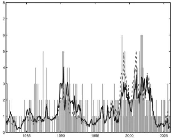
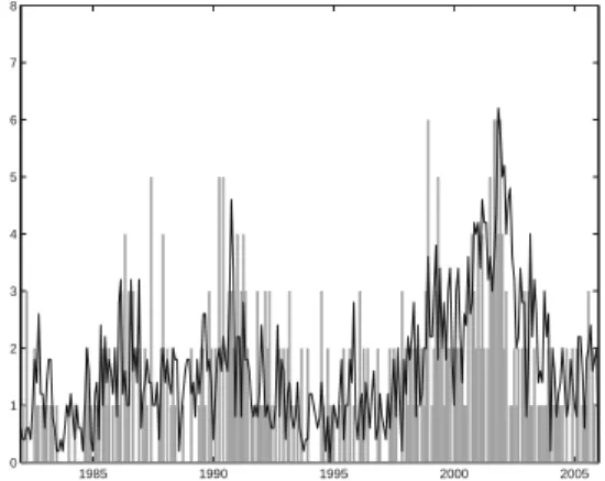
Figure I.1 shows monthly defaults along with the estimated cumulative default intensities for both models. Clearly, the estimated default intensities are different, but the graph also shows that it is difficult from visual inspection to tell which model gives the better fit.

We have examined the influence of additional economy-wide factors besides those appearing in Model I and II through proxies for the U.S. unemployment rate, the wages of U.S. production workers, the U.S. consumer price index, the U.S. gross domestic product in both real and nominal terms, the price of crude oil, and the spread between Moody’s Aaa-and Baa-rated corporate bonds, but without finding any significant effects. In a similar fashion, we have looked at a variety of alternative indicators of financial soundness at the firm-specific level including some of the empirical default predictors proposed by Altman (1968) and Zmijewski (1984), but likewise without finding support for further expansion of the set of explanatory variables.

Ideally, we should also take speciﬁc account of debt issue characteristics such as the time of issuance, maturity, face value, coupon payments including possible step up-clauses etc. given the empirical evidence presented in Davydenko (2010) who demonstrates the

7_{Duffie, Saita, and Wang (2007) suggest that this may in part reflect business cycle effects as well as be a}

consequence of correlation with the idiosyncratic stock returns, and perhaps also with other variables.

8_{Calculations are based on the likelihood ratio test statistic and its asymptotic distribution. However,}

the (asymptotically equivalent) Wald and score test statistics yield similar conclusions thus indicating a limited ﬁnite sample bias in the results.

(36)

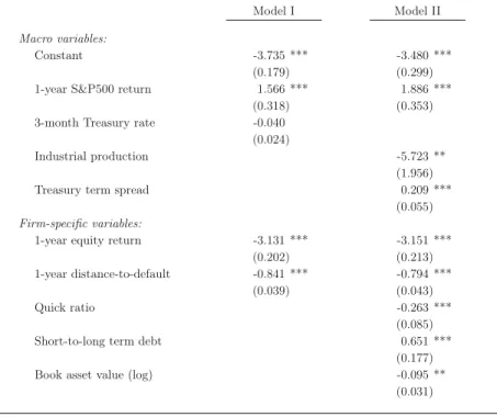
Table I.2. Parameter estimates (doubly stochastic models)

The macro variables entering the models are the 1-year return on the S&P500 index, the level of the 3-month U.S. Treasury yield, the 1-year percentage change in U.S. industrial production, and the spread between the 10-year and 1-year U.S. Treasury yields. The firm-specific variables are the 1-year stock return, the 1-year distance-to-default, the quick ratio, short-term debt as a percentage of total debt, and (log) book value of assets. Asymptotic standard errors are reported in parenthesis and statistical significance is indicated at 5% (*), 1% (**), and 0.1% (***) levels, respectively.8

Model I Model II

Macro variables:

Constant -3.735 *** -3.480 *** (0.179) (0.299) 1-year S&P500 return 1.566 *** 1.886 ***

(0.318) (0.353) 3-month Treasury rate -0.040

(0.024)

Industrial production -5.723 ** (1.956) Treasury term spread 0.209 ***

(0.055)

Firm-speciﬁc variables:

1-year equity return -3.131 *** -3.151 *** (0.202) (0.213) 1-year distance-to-default -0.841 *** -0.794 ***

(0.039) (0.043)

Quick ratio -0.263 ***

(0.085) Short-to-long term debt 0.651 ***

(0.177) Book asset value(log) -0.095 **

(0.031)

influence of this type of information on the probability of default. Similarly, it could also be of importance to allow for specific industry effects given the variation in default rates across industries documented by Li and Zhao (2006). However, the lack of available debt issue information and the limited number of defaults unfortunately prevents us from performing either type of analysis on the current data set. Working with larger data sets and performing out-of-sample tests would naturally lead us to include more variables but

(37)

I.3 Testing for conditional independence and contagion

Figure I.1. Aggregate default intensity 1982-2005

1985 1990 1995 2000 2005 0 1 2 3 4 5 6 7 8

Monthly number of U.S. industrial defaults recorded in Moody’s DRSD in the period 1982-2005 and estimated default intensities for the simple (Model I, dashed) and the expanded (Model II, solid) model.

as we will see in the next section our speciﬁcation is rich enough to capture the correlation in the data.

I.3 Testing for conditional independence and contagion

Having estimated the default intensities of each ﬁrm, we now follow DDKS and transform the time scale using the cumulative intensity and test whether on the new time scale the default arrivals are a unit rate Poisson process. We also propose and test an extended version of the default intensity which explicitly models the possibility of contagion through a Hawkes process speciﬁcation.

I.3.1 The time change test

The doubly stochastic assumption is meant to capture a setup in which probabilities of default of individual firms are affected by exogenous “background variables”. The variables are exogenous in the sense that they are not affected by actual defaults of firms. A helpful illustration from medical science could be pollution in a city and onsets of asthma attacks

(38)

among its citizens. When the level of pollution is high, there are more asthma attacks and hence onsets of these attacks are correlated. However, conditioning on the level of pollution the onsets are independent (assuming that asthma is non-contagious). Also, asthma attacks do not affect the level of pollution. For an example with more relevance to default modelling, it is possible that increasing oil prices will cause more firms who use oil as an input in their production to default, but that the defaults will have no effect on oil prices, so conditionally on the level of oil prices defaults are then uncorrelated. In models of stock returns, conditional independence is often assumed in factor models where the residual returns, i.e. the part that is not explained by the factors, are independent across firms.

The test procedure used in DDKS is easy to describe in fairly non-technical terms. First, estimate individual ﬁrm intensities using Cox regressions. Then compute the sum of these intensities. Under the assumption of orthogonality, i.e. that there are never exact simultaneous defaults, the sum of the intensities is equal to the aggregate default intensity. Now, transform time using the aggregate intensity and check whether aggregate defaults in the new time scale are a unit rate Poisson process. Testing this uses a range of diﬀerent properties of the Poisson process, such as moment properties and exponential waiting times between jumps.

To describe the test more rigorously, we ﬁrst recall that default times are said to be

orthogonal ifP(τi=τj) = 0wheneveri=j.The cumulative number of defaults among

nﬁrms is deﬁned as N(t) = n i=1 1₍_τ_i_≤_t₎ t≥0

and, as noted in the appendix, if the default times are orthogonal the cumulative default process has intensity

λ(t) =

n

i=1

λi(t)1(τi≥t) t≥0

and the compensator of the cumulative default process is then the integral of the intensity Λ(t) =

t

0 λ

(s)ds t≥0.

Hence, if we time-change the cumulative default process by the compensator, it follows from Meyer (1971) that the cumulative default process becomes a unit rate Poisson

(39)

I.3 Testing for conditional independence and contagion

process, i.e. the time-scaled process

J(t) =NΛ−1(t) t≥0

is then a unit Poisson process with jump timesVi= Λ(τ(i)), where0≤τ(1)≤τ(2)≤. . .

denotes the ordered default times. A consequence of this is that V1,V2−V1,. . . are

independent exponentially distributed variables and for any c > 0, the binned jump

times Zj= n i=1 1_]_c₍_j₋_1),_cj_](Vi)

will be independent Poisson(c)−distributed variables. In summary, if default times are

orthogonal, we can transform the time scale of the cumulative default process to obtain a unit rate Poisson process and we can then use standard properties of this process for testing. Note that conditional independence or the doubly stochastic assumption is not needed to have orthogonality of the default times. Thus, we really use the time transformation test as a misspeciﬁcation test. We return to this point in section I.4.

To test whether the default arrivals on the transformed time scale truly follow a unit rate Poisson process, we use various theoretical properties of such a process: that the number of arrivals in a time interval is Poisson distributed with a mean equal to the length of the time interval, that waiting times between jumps are exponentially distributed, that arrivals in disjoint time intervals are independent, and some moment properties.

If we split up the entire time period into intervals in each of which the cumulative

intensity increases by an integerc, then the number of arrivals in each of these intervals

are independent and Poisson distributed with meanc. We follow DDKS and refer tocas

the bin size, since it reﬂects the expected number of defaults in each time interval. The

largercis, the smaller is the total numberkof time intervals (and hence Poisson variables)

that we get, thereby weakening the power of our statistical tests. On the other hand, by

increasingcwe can hope to get a clearer picture of the presence of heavy tails representing

excess clustering of defaults. We use the same test statistics as those of DDKS, i.e. the

Fisher Dispersion (FD) and the upper tail statistics (UT1, UT2)9, and supplement with

further tests detailed in Karlis and Xekalaki (2000). Since we only have a limited number 9_{We correct for the apparent misprint in DDKS in the description of the upper tail median statistic by}

comparing the simulated median statistics to the samplemedian(instead of the sample mean). However, this implies that the median statistic by construction only will be eﬃcient for large bin sizes.