Procedia Economics and Finance 15 ( 2014 ) 19 – 26
2212-5671 © 2014 The Authors. Published by Elsevier B.V. This is an open access article under the CC BY-NC-ND license (http://creativecommons.org/licenses/by-nc-nd/3.0/).
Selection and peer-review under responsibility of the Emerging Markets Queries in Finance and Business local organization doi: 10.1016/S2212-5671(14)00441-9
ScienceDirect
Emerging Market Que
Post-crisis CDO valuatio
Gabriel G
aFinance Department, Bucharest University of EconomicAbstract
We propose a CDO valuation model with default intensit with Archimedean copulas. The model has been adap implemented a two steps process to calibrate the model consider an non-homogenous portfolio and model the companies and time. Second, we used a constrained simulation. Our approach provides a good approximation copulas.
© 2013 Published by Elsevier Ltd. Selectio Markets Queries in Finance and Business l Keywords:Archimedean copula; CDO;CDS; default intensities; d
1.Introduction
The market standard tool for pricing CDOs is 2000. In this setting the univariate distribution of t and then the joint distribution is specified using a on risk dependency modeling has evolved around the c proposed such as t-copula by O’Kane and Schö
* Corresponding author. Tel.: +40-744-361-435. E-mail address:[email protected].
eries in Finance and Business
on with Archimedean copulas
Gaiduchevici
a,*
c Studies, 13-15 Mihai Eminescu St., 010511 Bucharest, Romania.
ties derived from CDS quotes and dependence structure modeled pted to accommodate the after crisis market conditions. We l to replicate iTraxx Europe Series 15 tranche quotes. First we e loss process by letting default intensities vary both across d optimization technique to determine copula parameters via n of market data and allows for performance comparison between
on and peer review under responsibility of Emerging ocal organization
dependence structure.
the one factor Gaussian copula model introduced by Li, time to default for each asset is derived from market data ne factor Gaussian copula. The literature concerning credit copula concept. Many different types of copulas have been ögl, 2005, double t-copula by Hull and White, 2004 or © 2014 The Authors. Published by Elsevier B.V. This is an open access article under the CC BY-NC-ND license
(http://creativecommons.org/licenses/by-nc-nd/3.0/).
Archimedean copulas byHofert and Scherer, 2011. A method for inferring the copula parameters from market data was introduced by Hull and White, 2006.
In this study we propose a CDO valuation model based on default intensities calibrated to CDS quotes and credit risk dependence modeled with Archimedean copula functions. For the empirical study we used iTraxx Europe Series 15 data, retrieved from the Bloomberg database. The analysis was conducted on after the crisis data which led to supplemental challenges due to the changes in quotation styles for CDO tranches. The paper is organized as follows. In Section 2 we introduce the CDO valuation model. In Section 3 we describe the implementation. Section 4 presents the results and concludes.
2. CDO valuation
We assume the existence of a filtered probability space ሺȳǡ ࣠ǡ Էሻwhere Է is a pricing measure calibrated to market quotes. The reference portfolio is comprised of ݅ ൌ ͳǡ ǥ ǡ ܫ companies and their times to default are given by a positive random variable ߬. The default status of each entity is specified via an intensity model. The intensity used to derive the default probabilities is assumed to be a deterministic, nonnegative function denoted by ߣሺݐሻ. The term structure of survival probabilities,ҧሺݐሻ is related to ߣሺݐሻ by:
ҧሺݐሻ ൌ ݁ݔ ቆെ න ߣሺݑሻ݀ݑ ௧
ቇ
(1)
In the following we adopt the canonical model for constructing ߬ as it is implemented by Schönbucher, 2003 for its suitability to simulation. If, the variables ܷ are uniformly distributed in ሾͲǡͳሿ then:
߬ൌ ݂݅݊ሼݐ Ͳǣ ҧሺݐሻ ܷሽ (2)
The default times, ߬, are obtained by taking the inverse of the survival function at points ܷ. The greatest challenge in modeling the portfolio loss process is to determine the joint distribution of the times to default. We have used the copulas listed in Table 1, both in their exchangeable and nested forms, to introduce dependence among the stopping times by making the trigger variables ܷdependent. Results generated from a 1-parameter Gaussian copula are also presented for comparison reasons as this is the standard market model.Archimedean copulas are related to the Laplace transforms of univariate distribution functions. According to Joe, 1997 if we denote by ॷ the class of Laplace transforms that consist of strictly decreasing differentiable functions than the function ܥǣ ሾͲǡͳሿௗ՜ ሾͲǡͳሿ defined as:
ܥሺݑଵǡ ǥ ǡ ݑǢ ߠሻ ൌ ߶ሼ߶ିଵሺݑሻ ڮ ߶ିଵሺݑௗሻሽǡ ݑଵǡ ǥ ǡ ݑௗא ሾͲǡͳሿ (3) is a d-dimensional exchangeable Archimedean copula where ߶ א ॷ is called the generator function and ߠ is
the copula parameter. Table 1 presents the selected copulas and parameters relevant to this study. Table 1.Parameter space, generator and inverse generator functions and Kendall’s tau coefficients.
Family ߠ ߶ሺݑǡ ߠሻ ߶ିଵሺݑǡ ߠሻ ߬ Gumbel ሾͳǡ λሻ ൫െݐଵ ఏΤ൯ ሺെ ݐሻఏ ሺߠ െ ͳሻ ߠΤ Clayton ሺͲǡ λሻ ሺͳ ݑሻିଵ ఏΤ ݑିఏെ ͳ ߠ ሺߠ ʹሻΤ Frank ሺͲǡ λሻ െ ൫ͳ െ ൫ͳ െ ݁ ିఏ൯ ሺെݑሻ൯ ߠ െ ቆ ݁ିఏ௨െ ͳ ݁ିఏെ ͳቇ ͳ Ͷሺܦଵሺߠሻ െ ͳሻ ߠΤ Joe ሾͳǡ λሻ ͳ െ ሺͳ െ ሺെݑሻሻଵ ఏΤ െ ൫ͳ െ ሺͳ െ ݑሻఏ൯ ஶ ͳ ൫݇ሺߠ݇ ʹሻሺߠሺ݇ െ ͳሻ ʹሻ൯Τ ୀଵ
A-M-H ሾͲǡͳሻ ሺͳ െ ߠሻ ሺሺݑሻ െ ߠሻΤ ൬ͳ െ ߠ ߠݑ
ݑ ൰ ͳ െ ʹሺߠ ሺͳ െ ߠሻଶሺͳ െ ߠሻሻ ͵ߠΤ ଶ Nested Archimedean copulas provide an efficient way to recursively define the dependence structure. However, fitting a fully nested structure to a large data set is unfeasible. As an alternative to the fully nested model, we can consider copula functions with arbitrary combinations at each level. The high dimensionality of our data set and the knowledge about sectorial repartition of the companies made us particularly interested in nested structures given by the following form:
ܥሺݑଵǡ ǥ ǡ ݑௗሻ ൌ ߶ൣ߶ିଵ൫߶ଵൣ߶ଵିଵሺݑଵଵሻ ڮ ߶ଵିଵ൫ݑଵௗభ൯൧൯ ڮ ߶ିଵ൫߶௦ൣ߶௦ିଵሺݑ௦ଵሻ ڮ ߶௦ିଵ൫ݑ௦ௗೞ൯൧൯൧ ൌ ߶ ߶ିଵቌ߶௦ ߶௦ିଵሺݑ௦ሻ ௗೞ ୀଵ ቍ ௌ ௦ୀଵ (4)
whereݑ௦א ሾͲǡͳሿǡ ݏ א ሼͳǡ ǥ ǡ ܵሽǡ ݈ א ሼͳǡ ǥ݀௦ሽ where ܵ is the dimension of the outer copula and ݀௦ with ܫ ൌ σௌ௦ୀଵ݀௦ is the dimension of the ݏ inner copulas. This copula has ܵ ͳ margins and it is easier to model
because the number of parameters,ܵ ͳ, is much smaller than ܫ. As demonstrated by McNeil, 2008 a sufficient condition for this structure to be a copula function is that ߠ ߠ௦ for any ݏ א ሼͳǡ ǥ ǡ ܵሽ. In order to
sample from the above mentioned copulas we implemented our own sampling algorithms based on the contributions ofMcNeil, 2008 and Hofert, 2008.
We assume an equally weighted CDO portfolio consisting of ܫ reference entities, ܬ tranches and maturity
ܶ. The payment schedule ࣮ ൌ ሼݐൌ Ͳ ൏ ݐଵ൏ ڮ ൏ ݐൌ ܶሽ denotes the specific dates on which the premium
payments are made. Taking account of the changes described above, we define ܲሺݐሻ as the expected principal
of tranche ݆ at time ݐ expressed as a percentage of initial tranche principal. The discount factors are ݀ሺݐሻ ൌ
݁ି௧, where ݎ is the continuously compounded interest rate and the spread ݏ
is the number of basis points
paid per year in order to buy protection on tranche ݆. A reference entity ݅ ൌ ͳǡ ǥ ǡ ܫ is deemed to default before time ݐ א ሾݐǡ ܶሿ, if ߬ ݐ. The portfolio loss process at time ݐ is given by:
ܮሺݐሻ ൌܮܩܦ
ܫ ͳሺ߬ ݐሻǡ ݐ א ሾݐǡ ܶሿ ூ
ୀଵ
(5)
whereܮܩܦ is the loss given default for all companies. The losses are absorbed by tranches in order of seniority. The losses incurred by a particular tranche ݆ ൌ ͳǡ ǥ ǡ ܬ, at time ݐ are determined by the attachment point, ܽ, and detachment point ݀. Therefore the remaining principal of tranche ݆ at time ݐ is given by:
ܲሺݐሻ ൌ ە ۖ ۔ ۖ ۓ ͳ ܮሺݐሻ ܽ ݀െ ܮሺݐሻ ݀െ ܽ ܽ൏ ܮሺݐሻ ݀ Ͳ ܮሺݐሻ ݀ (6)
The defaults may happen anywhere in ሾͲǡ ܶሿ however, in order to simplify the computation we discretize the time frame according to the payment schedule and defer all defaults that happen on or before time ݐ to
the middle of the interval ሾݐିଵǡ ݐሿ. The value of a CDO tranche is the present value of its expected cash flows, and it involves three terms. The present value of the expected regular spread payments is given by:
ܸܲܧܲൌ ॱ ݏοݐ݀ሺݐሻܲሺݐሻ
ୀଵ
൩ (7)
where οݐൌ ሺݐെ ݐିଵሻ. The present value of the expected accrual payments is given by:
ܸܲܧܣൌ ॱ ͲǤͷ ݏοݐ݀ሺͲǤͷ ݐିଵ ͲǤͷ ݐሻ ቀܲሺݐିଵሻ െ ܲሺݐሻቁ
ୀଵ
൩ (8)
The present value of the expected payoffs caused by defaults is given by:
ܸܲܧܦ ൌ ॱ ݀ሺͲǤͷ ݐିଵ ͲǤͷ ݐሻ ቀܲሺݐିଵሻ െ ܲሺݐሻቁ
ୀଵ
൩ (9)
Pricing a CDO involves determining the breakeven up-front fee that would make the present value of the payments equal to the present value of the payoffs. From the perspective of the protection buyer the breakeven up-front payment is given by:
ݑሺߠሻ ൌ ܸܲܧܦെ ܸܲܧܲோെ ܸܲܧܣோ (10)
where the superscript in ܸܲܧܲோ and ܸܲܧܣோ denote that ݏ has been replaced by the specific running-spread,
ݏோ, according to the specification of the deal. Assuming deterministic discount factors, (10) only requires the computation of the portfolio loss at each point of the payment schedule. Unfortunately, as can be seen from (6), the remaining principal ܲሺݐሻ is not a linear function of the individual loss indicator. As a consequence the expected trance principal cannot be determined analytically and has to be computed via simulation.
The purpose of the model is to calibrate the copula so that the computed breakeven up-front fees would reproduce as accurately as possible the values observed on the market. The main goal of the calibration is to minimize de cumulative absolute deviations of the computed up-front fees ݑሺߠሻ from the market up-front fees ݑெ with respect to the copula parameters ߠ:
ܦሺߠሻ ൌ ఏ หݑሺߠሻ െ ݑ ெห ୀଵ (11)
Model calibration was performed with respect to the Kendall’s tau parameter because it was efficient to minimize over a bounded parameter space. For the exchangeable Archimedean copulas we calibrated over one parameter while for nested copulas we calibrated over 2 parameters characterizing the strength of dependence in and out of sector. Minimization of the objective function with respect to one parameter was performed using the algorithm described by Brent, 2002 that uses a combination of golden section and parabolic interpolation. For the twoparameter copulas the multi-dimensional minimum of the objective function was computed using a box constraint optimization algorithm based on the BFGS methodology and
implemented by Nocedal and Wright, 2006. Our choice for the method is supported by the fact that it is a direct-search algorithm that uses only function values, does not require calculation of derivatives and admits linear constraints on parameters.
3. Implementation
CDO tranche pricing is based on the following Monte Carlo routine:
Step 1. Specify all input parameters. The empirical part of this study was carried out on the iTraxx Europe Series 15 index which is comprised of the most liquid 125 CDSs referencing European investment grade credits. Standardized tranches cover losses in the ranges of Ͳ െ ͵Ψǡ ͵ െ Ψǡ െ ͻΨǡ ͻ െ ͳʹΨǡ ͳʹ െ
ʹʹΨand ʹʹ െ ͳͲͲΨ. Consequently, the number of companies ܫ ൌ ͳʹͷ, the number of tranches ܬ ൌ ͷ and the attachment and detachment points ሾܽǡ ݀ሿ are set according to the loss ranges provided by the first 5 tranches. The ܮܩܦ is set at 0.6 except for the case where it is implied by market quotes. The payment schedule ࣮ is set to match the regular payment dates with ܭ ൌ Ͷܶand ܶ ൌ ͷ. For each of the analyzed days we took the observed market up-front fees ݑெ and the zero interest rates needed to compute the discount factors ݀ሺݐሻ. For the particular case of Series 15 the first 5 tranche running-spreads expressed in basis points are ݏோൌ
ሼͷͲͲǡͷͲͲǡ͵ͲͲǡͳͲͲǡͳͲͲሽ. We made use of the fact that default correlation tends to be higher for the companies pertaining to the same industry sector and divided the portfolio into ܵ ൌ ͺ sectors according to their classification in Bloomberg database. At each iteration we performed ܰ ൌ ͳͲହ simulations. Calibration was performed for several days while Series 15 was on-the-run but only the results for 06-01 and 2011-09-30 are presented. Conclusions were drawn based on results generated for all calibrated days.
Step 2. Given ߣ and ࣮ we computed the survival probabilities ҧሺݐሻ as indicated in (1).
Step3. For each of the ܰ simulations we sampled ሺܷǡ ǥ ǡ ܷூሻ from one of the chosen copula types parameterized with ߠ. Then we computed the default times ߬ according to (2) and based on them we calculated the portfolio loss ܮሺݐሻ for each of the points in the payment schedule as indicated in (5). Having the portfolio loss profile, for each tranche ݆ and each ݐ compute the remaining tranche principal ܲሺݐሻ as described in (6).
Step 4.Having ܲሺݐሻ for each of the Monte Carlo iterations compute the present value of the regular spread payments, the accrual payment and the payoffs in case of default as in (7), (8), (9) and take the expectation as their sample means.
Step 5. Compute the up-front fees as in (10) with the sample means generated at Step 4. Step 6. Repeat Step 1 – Step 5 with different ߠ so that measure ܦ is minimal.
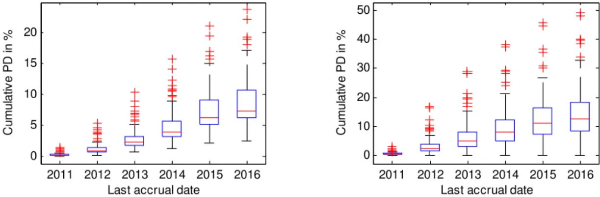
In order to model the loss process we consider an inhomogenous portfolio by letting default intensities vary both across companies and time. To determine the step function of hazard rates we have used the term structure of CDS spreads up to 5 years. The idea behind this procedure is that given the term structure of the hazard rate that is complete up to time ݐ െ ͳ, find the hazard rate at time ݐ that is consistent with de CDS spread at time ݐ. To apply this procedure we have implemented our own numerical root-finding algorithm based on Newton-Raphson method. The spread is an increasing function of hazard rate and we also assumed that this relation is linear. In general the algorithm is very fast because the convergence is quadratic, however the execution time is significantly influenced by the initial guess from which the algorithm starts. We mentioned this aspect because there is significant variability in CDS spreads across companies. To determine the unconditional default probabilities (PD) at each ݐwe numerically integrated over the term structure of the hazard rates. Figure 1 presents the result and gives a clear indication that in order for a copula to accurately describe the dependence structure it should provide enough tail dependency to catch the extreme co-movement of the variables.
Fig.1. (a) Distribution of unconditional cumulative PDs for all companies in the portfolio as seen from 2011-06-01; (b) Distribution of unconditional cumulative PDs for all companies in the portfolio as seen from 2011-09-30.
4. Results and Conclusions
Our objective was to replicate all tranche prices simultaneously by calibrating over the parameter space of the copula in order to minimize the measure ܦ. Results generated after calibrating for all types of copulas indicated that the model is consistent across time despite the significant changes in the credit market. Credit conditions worsened during 2011 on the background of stagnating European economy and deteriorated perception on sovereign creditworthiness. Tables2 and 3 present the estimated tranche up-front fees and measure ܦ for 2011-06-01 and 2011-09-30 respectively. We chose to present these dates in detail as they clearly reflect model consistency through different market conditions.
A crucial aspect regarding calibration is that up-front payments for junior tranches are inversely correlated with the dependence among firms. However, this is exactly the opposite with senior tranche as their up-front fees are positively correlated with the dependence among firms. We have observed a tendency for the model to overprice senior tranches. Constant overpricing of senior tranches has several justifications. First, we calibrate the copula so as to reflect the overall portfolio credit dependency. Since the highest up-front fee is paid for tranches Ͳ െ ͵Ψ and ͵ െ Ψ it is normal that they would have the highest influence in determining the credit dependence. This overestimation of default dependence induced by the first two tranches extrapolates by increasing the risk, and therefore the price, for the senior tranches. Second, the periodic payments for all tranches are arbitrarily determined by the running-spread. Since superior tranches have significantly lower running-spreads than junior tranches it is normal for the model to compensate by increasing the up-front fee. Third, the market itself may be inefficient in pricing superior tranches. This belief is based on the fact that investors are more concerned with correctly pricing junior tranches as these have a higher probability of being hit by defaults and don’t manifest the same diligence when pricing superior tranches. Therefore, we may conclude that the model performs consistently across tranches.
Among the 5 Archimedean copula families the two parameter Gumbel copula performed best. This was also our a priori expectation because Gumbel copula exhibits upper tail dependence, that is, it is more suitable to describe outcomes that simultaneously produce upper tail values. Joe copula performed well and close to Gumbeland therefore we consider it suitable for this type of analysis. This consideration is intuitive as they have the same tail characteristics and parameters spaces.Except for the Gumbel copula, all the copula classes do not materially improve the performances of the model by calibrating over 2 parameters instead of one. This provides a solid reason to conclude that it is the structure of (tail) dependence that matters most and not a particular value of the parameter.
Table 2.Calibrated copula parameters and tranche up-front fees for 1st of June 2011. 2011 2012 2013 2014 2015 2016 0 5 10 15 20
Last accrual date
C u mu la tiv e P D in % 2011 2012 2013 2014 2015 2016 0 10 20 30 40 50
Last accrual date
C u mu la tiv e P D in %
2011-06-01 Trance up-front fees (%) ࡰ Kendall’s tau 0-3% 3-6% 6-9% 9-12% 12-22% Market 38.25 4.60 1.87 1.94 0.91 Gauss 1 0.28 39.79 4.73 6.05 7.59 2.42 13.00 Gumbel 1 0.31 37.68 3.00 3.4 3.26 2.04 6.15 Gumbel 2 0.24 0.39 37.69 4.91 2.45 3.38 1.75 3.72 Survival Clayton 1 0.14 36.98 9.86 6.68 6.08 2.09 16.65 Survival Clayton 2 0.12 0.21 36.25 9.01 6.32 5.53 2.22 15.75 Frank 1 0.43 37.67 8.04 5.95 8.83 2.61 16.68 Frank 2 0.42 0.45 38.09 8.25 6.01 8.84 2.36 16.28 AMH 1 0.33 47.04 18.92 7.83 6.46 1.69 34.36 AMH 2 0.30 0.33 48.16 17.6 7.91 5.85 1.90 33.84 Joe 1 0.24 39.35 4.35 2.76 5.16 2.16 6.71 Joe 2 0.170.32 37.91 4.03 1.20 4.42 1.16 4.31
Table 3.Calibrated copula parameters and tranche up-front fees for 30th of September 2011.
2011-09-30 Trance up-front fees (%)
ࡰ Kendall’s tau 0-3% 3-6% 6-9% 9-12% 12-22% Market 61.44 27.65 19.14 4.91 2.34 Gauss 1 0.40 59.63 28.41 24.07 14.01 9.62 23.87 Gumbel 1 0.39 62.20 27.03 21.92 6.70 5.29 8.89 Gumbel 2 0.34 0.48 61.24 27.83 19.73 6.24 4.72 4.67 Survival Clayton 1 0.26 54.54 27.69 22.81 20.32 13.73 37.40 Survival Clayton 2 0.22 0.28 58.27 31.16 24.70 16.99 11.5 33.47 Frank 1 0.43 62.76 30.56 24.22 23.98 13.65 39.68 Frank 2 0.42 0.5 58.80 30.01 24.36 24.31 10.77 38.04 AMH 1 0.30 77.14 33.53 24.51 17.93 9.78 47.40 AMH 2 0.30 0.33 76.99 32.50 25.42 19.06 10.03 48.51 Joe 1 0.35 61.30 28.53 21.51 10.51 5.35 11.99 Joe 2 0.24 0.52 61.55 27.05 20.17 7.74 5.97 8.19
Clayton copula, even though it was used in the survival form showed weak performance and therefore sustains the fact that it is not suitable in this modeling context. This is also the only copula that has a tendency to fit in between, that is, to underprice junior tranches and overprice senior ones.AMH and Frank copulas, as expected, performed worst due to their lack of tail dependence. In addition AMH has a restricted parameter space which prevents it from capturing enough dependence. This is the reason why calibrated parameters for the AMH copula came very close to the upper limit of the parameter space. Even though calibrations for exchangeable and nested copulas were independent the parameter calibrated in the exchangeable form always falls between the parameters calibrated for the nested form. This leads us to conclude that information about sectorial repartition has a significant influence on the dependence structure. Even more so, for every copula and every calibrated day the inter sector parameter was lower than the intra sector one. This reinforces our belief that dependence among companies is clustered according to industry sectors. The naïve Gaussian model does not properly capture the dependence characteristics of the portfolio. What is even more discouraging to using this type of copula in this context is that its performance decreases as dependence among companies increases. This finding is supported by the fact that it performed worst in relative terms during the analyzed time period that exhibited worsening credit conditions and increasing dependence.
Acknowledgements
This work was co-financed from the European Social Fund through Sectoral Operational Programme Human Resources Development 2007-2013; project number POSDRU/107/1.5/S/77213 „Ph.D. for a career in interdisciplinary economic research at the European standards”
The scientific support and access to databases provided by Ladislaus von Bortkiewicz Chair of Statistics, C.A.S.E. - Center for Applied Statistics and Economics, Humboldt-Universitätzu Berlin is gratefully acknowledged.
References
Li, D.X., 2000.On Default Correlation: A Copula Function Approach. The Journal of Fixed Income, 9, 4, p. 43-54.
O’Kane, D.,Schögl, L., 2005.A note on the large homogenous portfolio approximation with the Student-t copula.Finance and Stochastics, 9(4), p. 577-584.
Hull, J., White, A., 2004. Valuation of a CDO and an nth to default CDS without montecarlo simulation. Journal of Derivatives 12 (2), p. 8–23.
Hofert, M., Scherer, M., 2011. CDO pricing with nested Archimedean copulas. Quantitative Finance 11(5), p. 775–787. Hull, J., White, A., 2006. Valuing credit derivatives using an implied copula approach. Journal of Derivatives 14(2), p. 8–28. Schönbucher, P., 2003. Credit Derivatives Pricing Models: Model, Pricing and Implementation. John Wiley & Sons. Joe, H., 1997. Multivariate Models and Dependence Concepts.Chapman & Hall, London.
McNeil, A., 2008. Sampling nested Archimedean copulas. Journal Statistical Computation and Simulation 78(6), p. 567–581. Hofert, M., 2008.Sampling Archimedean copulas. Computational Statistics & Data Analysis 52(12), p. 5163–5174. Brent, R., 2002. Algorithms for Minimization without Derivatives.Prentice-Hall.