failure”
AUTHORS A. Blanco-Oliver A. Irimia-Dieguez M.D. Oliver-Alfonso M.J. Vázquez-Cueto ARTICLE INFOA. Blanco-Oliver, A. Irimia-Dieguez, M.D. Oliver-Alfonso and M.J. Vázquez-Cueto (2016). Hybrid model using logit and nonparametric methods for predicting micro-entity failure. Investment Management and Financial Innovations, 13(3), 35-46. doi:10.21511/imfi.13(3).2016.03
DOI http://dx.doi.org/10.21511/imfi.13(3).2016.03
JOURNAL "Investment Management and Financial Innovations"
FOUNDER LLC “Consulting Publishing Company “Business Perspectives”
NUMBER OF REFERENCES
0
NUMBER OF FIGURES0
NUMBER OF TABLES0
A. Blanco-Oliver (Spain), A. Irimia-Dieguez (Spain), M.D. Oliver-Alfonso (Spain), M.J. Vázquez-Cueto (Spain)
Hybrid model using logit and nonparametric methods for predicting
micro-entity failure
Abstract
Following the calls from literature on bankruptcy, a parsimonious hybrid bankruptcy model is developed in this paper by combining parametric and non-parametric approaches.To this end, the variables with the highest predictive power to detect bankruptcy are selected using logistic regression (LR). Subsequently, alternative non-parametric methods (Multilayer Perceptron, Rough Set, and Classification-Regression Trees) are applied, in turn, to firms classified as either “bankrupt” or “not bankrupt”. Our findings show that hybrid models, particularly those combining LR and Multilayer Perceptron, offer better accuracy performance and interpretability and converge faster than each method implemented in isolation. Moreover, the authors demonstrate that the introduction of non-financial and macroeconomic variables complement financial ratios for bankruptcy prediction.
Keywords: bankruptcy models, combining forecasts, decision making, hybrid models, data mining, small firms.
JEL Classification: G33, C53.
Introduction ©
The financial crisis has spiked interest in empirical research in corporate bankruptcy prediction. Many different models have been used to predict corporate failure; nevertheless, to select the most appropriate for empirical applications is not straightforward. Data mining algorithms (DMAs) have recently fitted failure models with higher predictive power than the traditional methods, such as discriminant analysis (DA) and logistic regression (LR). The boom of DMAs is substantiated by the capacity of these algorithms to work effectively in non-linear environments where the presence of a high level of noise and a low sample sizeis strong (Marquez et al., 1991). Additionally, the assumptions of parametric approaches such as DA or LR might not hold true in many cases. The requirements of linearity, normality and independence among input variables, and the establishment of a strict functional form in the relation between predictive and response variables, limit real world applications (Eisenbeis, 1977; Karels and Prakash, 1987). Nevertheless, many DMAs (e.g., Neural Network) are black-box methods and, therefore, are difficult, if not impossible, to interpret. Furthermore, parametric approaches do allow us to determine the sense (positive or negative) and the importance (e.g., p
© A. Blanco-Oliver, A. Irimia-Dieguez, M.D. Oliver-Alfonso, M.J. Vázquez-Cueto, 2016.
A. Blanco-Oliver, Department of Financial Economy and Operations Management, Faculty of Economics and Business Sciences, University of Seville, Spain.
A. Irimia-Dieguez, Department of Financial Economy and Operations Management, Faculty of Economics and Business Sciences, University of Seville, Spain.
M.D. Oliver-Alfonso, Department of Financial Economy and Operations Management, Faculty of Economics and Business Sciences, University of Seville, Spain.
M.J. Vázquez-Cueto, Department of Applied Economics III, Faculty of Economics and Business Sciences, University of Seville, Spain.
value) of how the input variables affect firm bankruptcy, although certain relevant proposals exist for knowing more about the sense and importance of input variables in DMAs, among which the Bayesian neural networks stand out. In recent years, a research approach has emerged which combines both parametric and non-parametric techniques to fit hybrid failure models (e.g., Chen 2011; Chen et al., 2011; Jagric et al., 2011; Sánchez-Lasheras et al., 2012; Rodrigues and Stevenson, 2013). However, these models have not been widely employed in prior studies despite the fact that theoretical principles and the existing empirical evidence suggest the superiority of hybrid models over single-type models to predict firm bankruptcy. The implementation of both parametric and non-parametric statistical approaches minimizes the theoretical problems of each technique in isolation, also providing effective synergies between them (Castro et al., 2014). According to previous studies (Timmermann, 2006; Fan et al., 2011; Rodrigues and Stevenson, 2013), hybrid models have better interpretability (the most relevant input variables and their estimator sign are known), reduce the dimension and accelerate the convergence rate while dealing in a non-linear and non-parametric adaptive-learning environment. In this framework, the main objective of this paper is to build and compare the performance of several parsimonious bankruptcy models focused on micro-entities1 (MEs), by considering financial, non-financial and macroeconomic information, and by employing different hybrid models which are applied in two
1 MEs constitute a very relevant firm size which has recently been
defined in the Directive 2012/6/EU as those companies which do not exceed the limits of two of the three following criteria: (a) total assets of €350,000; (b) annual turnover of €700,000 and; (c) average number of employees during the financial year of 10.
steps. First, the traditional LR (parametric approach) is applied. Second, the following non-parametric methods are performed: (1) multilayer perceptron neural networks (MLP) (Neves and Vieira 2006; Angelini et al., 2008); (2) rough sets (RS) (Slowinski and Zopounidis, 1995; Dimitras et al., 1999); and (3) classification and regression trees (CART) (Gepp et al., 2009). We compare the performance of several hybrid failure models based on DMAs since, as explained in Witten and Frank (2005), the different data mining methods correspond to different concept description spaces searched with different schemes. In this sense, MLPs are consistent with the universal approximation property whilst permitting a high level of noise and low sample size (Gibbons and Chakraborti, 2014). CART, likewise, uses a nonlinear procedure, and also provides interpretable results.
This paper updates the literature in three ways. First, we provide a new approach – a hybrid model – for developing bankruptcy models which exploits the advantages of both parametric and non-parametric methods by creating synergies and minimizing the cost associated with the implementation of each method in isolation. Second, we use a highly relevant and recently defined firm size which represents over 75 per cent of European Union businesses and 30 per cent of the European work force. To the best of the authors’ knowledge, our bankruptcy model is the first specifically designed for this firm size. The existing failure models – routinely built based on numerous finance-accounting ratios – cannot be applied to MEs, because their reporting regimen does not require this financial information. Third, in accordance with recent research (e.g., Altman et al., 2010), we test the predictive power added by the introduction of non-financial and macroeconomic information as predictor variables in the development of bankruptcy models. In this regard, bankruptcy literature suggests that the financial ratios are not really predictor variables of the financial distress of a firm, but are the observable and measurable output of these financial problems. Therefore, financial ratios can only detect the financial distress of a firm in near bankruptcy, and should, therefore, be complemented by the non-financial and macroeconomic data which are well recognized as efficient early warning variables. The influence of directors’ management skills and family character on the performance of firms (Wilson et al., 2013), along with the positive relationship between the adverse economic cycle and the number of corporate failures (Moon and Sohn, 2010), represent two examples of the substantial importance of non-accounting data on failure prediction.
In section 1, we provide details of our UK sample, and examine in detail the data routinely available to model small enterprise failure amongst unlisted firms. Section 2 develops several failure prediction models for micro-entities and explains the methodologies applied. Section 3 applies the models to sample forecasts and discusses the results. Final section provides the main conclusions and proposes future lines of research.
1. Data
1.1. Description of firm-population: micro-entities. In 2003, the European Commission Recommendation 2003/361/EC classifies the smallest companies into three segments: micro, small and medium-sized enterprises, although consultations with Member States suggested a sub-group of the smallest micro-enterprises, MEs, to represent companies with a size lower in both total balance sheet and net turnover than that laid down for micro-enterprises. In 2012, the European Parliament (Directive 2012/6/EU) redefined the enterprises sizes including MEs resulting in four groups of SMEs: micro-entities, micro, small and medium-sized enterprises. The major quantitative relevance of MEs in the United Kingdom represent approximately 42% of all companies (BIS, 2013) and their homogeneous characteristics and challenges, justified the creation of this new, size-based classification.
Their most relevant features and problems are linked to financial and legal issues, ownership structure and type of management, and limited resources. Traditionally, they experienced excessive difficulties when attempting to access funding sources, owing to high asymmetry problems between MEs and lenders. They are considered opaque with regards to financial information; publically available financial data are usually limited and unreliable given unaudited accounts (Berger and Frame, 2007). Other factors that influence this funding constraint are the lack of access to capital markets, of credit ratings, and MEs’ track record of high bankruptcy rates (Ciampi and Gordini, 2013). The figure of owners and directors coincide and casts doubt on the reliability of financial ratios (Claessens et al., 2000). These arguments support the consideration of MEs as a new business size that requires differentiated treatment. The European Directive 2012/6/EU not only created the micro-entity firm size, but also more importantly, established a new simplified financial reporting regime soughing to reduce the administrative burden of statutory reporting. This new accounting regime introduced a set of exemptions for MEs from the accounting requirements of the 4th and 7th Directives. To
introduce these exemptions in the UK – the country analyzed in the present study – the Government published The Small Companies (Micro-entities’ Accounts) Regulations 2013, under which the MEs need to file, at the official business register, only a simple balance sheet with information disclosed at the foot. This new accounting regimen may compound an information asymmetry problem, and maybe the reason a proportion of UK micro and small companies filling full, audited accounts voluntarily (Collis, 2012). In this context, the need arises for the development of failure models specifically designed for the intrinsic characteristics (only using limited financial data contained in the new financial reporting regime under Directive 2012/6/EU) of MEs, since, to date, no bankruptcy models have yet been built specifically for this firm size. Very small enterprises account for most economic activity worldwide and have traditionally experienced a higher probability of failure than large corporations (Carter and Van Auken, 2006). The models developed in this paper should reduce the high informational gap that ME shareholders (mainly investors, lenders and suppliers) face, and thus, improve the decision-making process.
1.2. The dataset and explanatory variables. A dataset provided by a U.K. Credit Agency is used in this study2. After eliminating missing and abnormal (which lie within the top 1% and the bottom 1% of each financial ratio) cases, we select a random sample of MEs, with 39,710 sets of accounts remaining (50% non-failed) for1 the period 1999-20083. In line with other studies, we2define corporate failure as entry into liquidation, administration or receivership in the analyzed period. The accounts analyzed for failed companies are the last set of accounts filed in the year preceding insolvency. For each case, the dependent variable (corporate failure) takes the value 1, when the ME failed and 0, otherwise.
To estimate the prediction error (generalization error) of the models developed here on new data (model assessment), we follow Hastie et al. (2009), and our final dataset was randomly split into three sub-sets4: a training set of 60%, a3 validation set5 of 20% and a test data set (or hold-out sample) of420%.
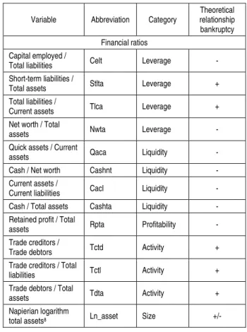
Table 1 describes the variables considered in this study and the theoretical relationship with firm
2 The data set used in the present study was supplied under license
agreement and can not be made publicly available.
3 Table A.1 and A.2 of Appendix 1 summarize the descriptive statistics
of all variables for both the failed and non-failed samples.
4 Another argument that supports this division is the big size of our data
set (Hastie et al., 2009).
5 In the case of logistic regression, the optimal cut-off point is obtained
through the validation sub-sample.
failure. Motivated by MEs intrinsic characteristics of limited and sometimes unreliable financial information, we assume that an adequate bankruptcy model made specifically for MEs should not be based solely upon financial ratios. Therefore, as suggested in previous literature (e.g., Grunert et al., 2005; Altman et al., 2010; Wilson and Altanlar, 2013), we also include non-financial variables as explanatory inputs on the presumption that the combined use of both financial and non-financial variables increases the accuracy of the failure models built. Finally, a macroeconomic variable –
Industry solvency – which measures the financial
health of the sector in which the firm operates and is the inverse of the probability of bankruptcy for the sector, was also considered as an independent variable, since several studies have shown a positive relationship between an adverse economic cycle and the number of corporate failures (e.g., Moon and Sohn, 2010)6. 5
Table 1. Financial, non-financial and macroeconomic variables7 6
Variable Abbreviation Category
Theoretical relationship bankruptcy Financial ratios
Capital employed /
Total liabilities Celt Leverage -
Short-term liabilities /
Total assets Stlta Leverage +
Total liabilities /
Current assets Tlca Leverage +
Net worth / Total
assets Nwta Leverage -
Quick assets / Current
assets Qaca Liquidity -
Cash / Net worth Cashnt Liquidity -
Current assets /
Current liabilities Cacl Liquidity -
Cash / Total assets Cashta Liquidity -
Retained profit / Total
assets Rpta Profitability -
Trade creditors /
Trade debtors Tctd Activity +
Trade creditors / Total
liabilities Tctl Activity +
Trade debtors / Total
assets Tdta Activity +
Napierian logarithm
total assets8 Ln_asset Size +/-
6 For a detailed analysis of the variables employed here, see Altman et
al. (2010).
7 For more details about the non-financial variables, see Table A.3. of
Appendix A.
8 Many previous studies found that large firms are less likely to encounter
credit constraints thanks to the effect of a good reputation, and therefore their studies conclude that a firm’s small size may lead to insolvency (Dietsch and Petey, 2004). In contrast, Altman et al. (2010) find that the relationship between asset size and insolvency risk appears to be non-linear, since it is positive when the firms have less than £350,000 in assets, and is negative when their assets are higher than this value.
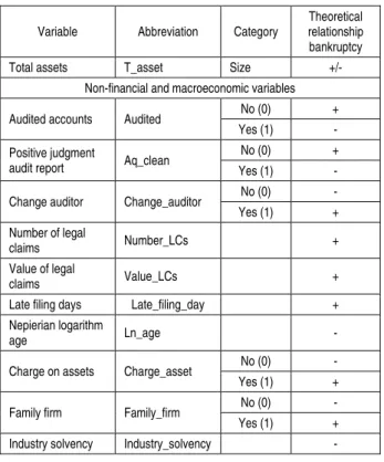
Table 1 (cont.). Financial, non-financial and macroeconomic variables
Variable Abbreviation Category
Theoretical relationship bankruptcy
Total assets T_asset Size +/-
Non-financial and macroeconomic variables
Audited accounts Audited No (0) +
Yes (1) -
Positive judgment
audit report Aq_clean
No (0) +
Yes (1) -
Change auditor Change_auditor No (0) -
Yes (1) +
Number of legal
claims Number_LCs +
Value of legal
claims Value_LCs +
Late filing days Late_filing_day +
Nepierian logarithm
age Ln_age -
Charge on assets Charge_asset No (0) -
Yes (1) +
Family firm Family_firm No (0) -
Yes (1) +
Industry solvency Industry_solvency -
2. Methods
2.1. Forecasting strategy and accuracy measuresof models. In theory, the non-parametric statistical techniques implemented here (MLP, RS and CART) should obtain higher accuracy performance than the classic parametric method (LR), although there is empirical evidence in both directions (Ravi Kumar and Ravi, 2007; Olson et al., 2012). This theoretical superiority is mainly supported by the high complexity, computational power, and learning capability associated with non-parametric approaches. Nevertheless, the transparency of the LR models in regards to variable selection and time structure, adds flexibility, allowing the researcher to adapt the model correspondingly (Rodrigues and Stevenson, 2013). Therefore, the use of hybrid models – combining both parametric and non-parametric approaches – should minimize the theoretical problems of each technique in isolation and provide effective synergies between them.
To exploit the above advantages, this study builds bankruptcy models in two steps. First, the LR method’s strengths are employed to select the most relevant variables, which also allows establishing the empirical relationship between these predictors and ME bankruptcy (through the signs of its coefficients). Second, by introducing only these significant variables, we implement each of three non-parametric techniques (MLP, RS and CART). From a theoretical point of view, this procedure should allow us to reduce the dimension and to
accelerate the convergence of non-linear methods, as well as to improve the interpretability and the accuracy performance of the resulting bankruptcy models. That is, with the implementation, first of LR, and, then, of a non-parametric model (hybrid failure model), it is possible to exploit the advantages of both statistical approaches.
In order to evaluate the performance of each model, we use the area under the ROC curve (AUC) and misclassification costs (MC) (West, 2000).
2.2. Logistic regression and selection of input variables. In this study, the LR model has been fitted with the glm function in R (Venables and Ripley, 2002) which strives to compute the maximum likelihood estimators of the n + 1 parameters by means of an iterative weighted least squares (IWLS) algorithm.
We use LR instead of other parametric methods (such as linear discriminant analysis, LDA) since several authors (including Karels and Prakash, 1987) point out that two basic assumptions of LDA are often violated when applied to default prediction problems. Moreover, it provides a suitable balance of accuracy, efficiency, and interpretability of the results, as affirmed by Crone and Finlay (2012). To select the most relevant explanatory variables, we apply several procedures with a sole objective: to build parsimonious failure models. To select the most relevant financial ratios, in accordance with Altman and Sabato (2007), we follow the steps outlined below. Once the potential candidate predictors have been defined and calculated, the accuracy ratio (AR) is observed for each financial variable9. To avoid the problem of multicollinearity between the independent variables of the model, only one variable is selected from each ratio category. The variable selected is that which has the highest accuracy ratio from each group. These five most significant variables, one from each accounting category, are, then, considered to create the first LR model (LR 1) which only introduces financial ratios. Table 2 shows all the financial ratios, the accounting category to which they pertain, and their AUC and AR values. 1
Table 2. Selected financial ratios Variable examined Accounting
ratio category AUC (%) AR (%) Variable selected Capital employed /
Total liabilities Leverage 69.10 38.20 X
Short-term liabilities / Total assets
Leverage 57.60 15.20
9 According to Engelmann et al. (2003), the accuracy ratio (AR) is
Table 2 (cont.). Selected financial ratios Variable examined Accounting
ratio category AUC (%) AR (%) Variable selected Total liabilities /
Current assets Leverage 67.10 34.20
Net worth / Total
assets Leverage 69.00 38.00
Quick assets /
Current assets Liquidity 59.80 19.60
Cash / Net worth Liquidity 51.10 2.20
Current assets /
Current liabilities Liquidity 66.70 33.40
Cash / Total assets Liquidity 69.40 38.80 X
Retained profit /
Total assets Profitability 70.00 40.00 X
Trade creditors /
Trade debtors Activity 57.20 14.40
Trade creditors /
Total liabilities Activity 54.40 8.80
Trade debtors /
Total assets Activity 61.60 23.20 X
Ln total assets Size 63.50 27.00 X
Total assets Size 63.20 26.40
To explore whether the non-financial information increases the accuracy performance of our model, the most relevant non-financial information is introduced into the previous model resulting in a new LR model (LR 2). To this end, a forward
stepwise selection procedure is implemented, thereby concluding that Number_LCs,
Late_filing_day, Ln_age, Family_firm and
Industry_solvency are the most significant
non-financial variables.
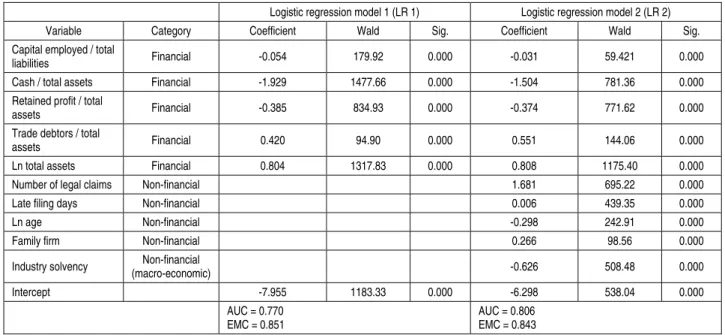
The coefficients and significance level of all variables considered in each model are collected in Table 3. As shown in this table, all slopes (signs) follow our expectations. The relevance of these variables on firm failure can also be analyzed by the absolute values of Wald ratio coefficients for each variable. Cash/total assets and Ln_asset are the most relevant variables in the model which considers only financial variables, whereas
Ln_asset, Cash/total assets and Number_ LCs are
the most relevant variables in the models which introduce non-financial variables (LR 2). Based on these results and in accordance with the present study’s objective, only the variables of the failure model with the highest capacity to detect ME bankruptcy (LR2) are used as input variables in the subsequent statistical methods (MLP, CART and RS) Table 5 of Section 4.1. analyzes the accuracy performance of each model and the predictive power added by each type of explanatory variable.
Table 3. Logistic-default prediction models for the micro-entities
Logistic regression model 1 (LR 1) Logistic regression model 2 (LR 2)
Variable Category Coefficient Wald Sig. Coefficient Wald Sig.
Capital employed / total
liabilities Financial -0.054 179.92 0.000 -0.031 59.421 0.000
Cash / total assets Financial -1.929 1477.66 0.000 -1.504 781.36 0.000
Retained profit / total
assets Financial -0.385 834.93 0.000 -0.374 771.62 0.000
Trade debtors / total
assets Financial 0.420 94.90 0.000 0.551 144.06 0.000
Ln total assets Financial 0.804 1317.83 0.000 0.808 1175.40 0.000
Number of legal claims Non-financial 1.681 695.22 0.000
Late filing days Non-financial 0.006 439.35 0.000
Ln age Non-financial -0.298 242.91 0.000
Family firm Non-financial 0.266 98.56 0.000
Industry solvency (macro-economic) Non-financial -0.626 508.48 0.000
Intercept -7.955 1183.33 0.000 -6.298 538.04 0.000
AUC = 0.770 EMC = 0.851
AUC = 0.806 EMC = 0.843
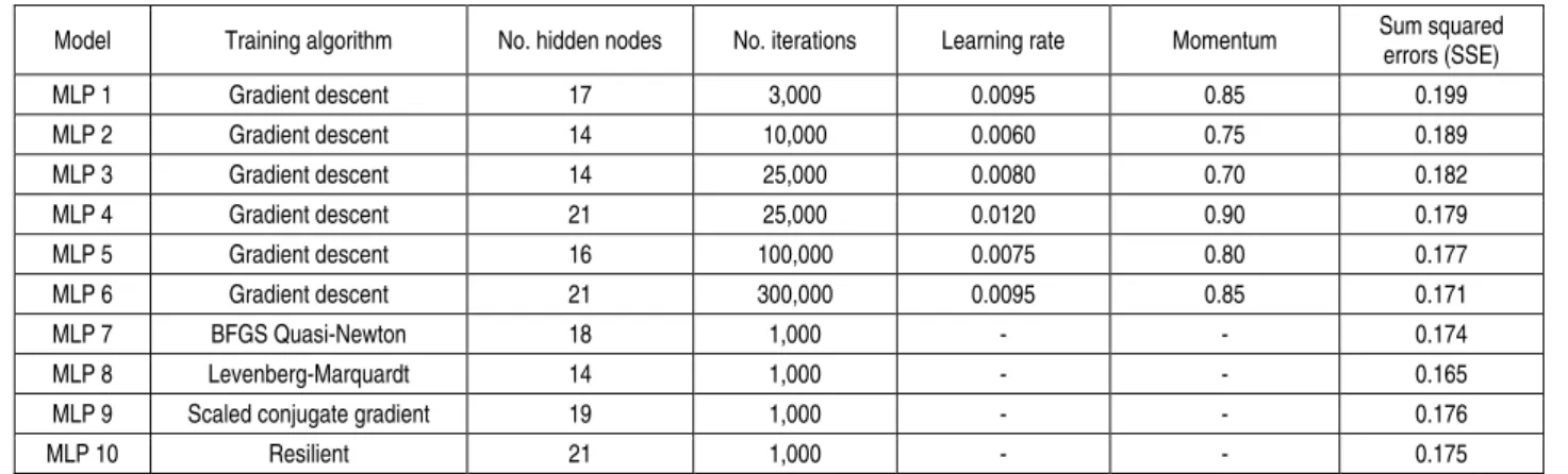
2.3. Non-parametric approaches. 2.3.1. Multilayer
perceptron. An MLP is a neural network typically
comprised of at least three different layers: an input layer, one or more hidden layers, and an output layer (Rumelhart et al., 1986). The number of nodes in the input layer corresponds to the number of predictor variables, and the number of nodes in the output layer to the number of dependent variables. Nevertheless, the number of hidden layers and the number of hidden layer nodes are more problematic to define. In the case of the number of hidden layers, the universal
approximation property of MLP states that one hidden-layer network is sufficient to model any complex system with any desired level of accuracy (Zhang et al., 1998), thus, all our MLPs will have only one hidden layer. Finally, the most common way to determine the size of the hidden layer is via experiments or trial and error (Wong, 1991). The basic parameters of all MLP-based models built are explained below and summarized in Table 5. For the gradient-descent training rule, Rumelhart et al. (1986) concluded that lower learning rates tend to give the
best network results, and that the networks are unable to converge when the learning rate is greater than 0.012. Moreover, in previous research, it is common to test various learning rates and to choose that for which network performance is the best. Therefore, learning rates 0.006, 0.0075, 0.008, 0.0095, and 0.012 are tested during the training process. Another relevant parameter is momentum. In our study, as is recommended by MATLAB (which was used to perform all the MLP experiments), momentum ranges from 0.70 to 0.90. The network weight is reset for each combination of the network parameters, such as
learning rates and momentum. For the stopping criteria of MLP, this study allows a maximum of 3,000, 10,000, 25,000, 100,000, and 300,000 learning epochs per training10 second-order training methods are used, the maximum learning epochs per training allowed is 1,000. The network topology with the minimum testing SSE is considered as the optimal network topology. In summary, ten MLP-based models are developed. The first six MLPs are fitted by using the traditional gradient-descendent training algorithm, while the other four MLPs employ second-order training algorithms.
Table 4. Multilayer perceptron models
Model Training algorithm No. hidden nodes No. iterations Learning rate Momentum Sum squared
errors (SSE) MLP 1 Gradient descent 17 3,000 0.0095 0.85 0.199 MLP 2 Gradient descent 14 10,000 0.0060 0.75 0.189 MLP 3 Gradient descent 14 25,000 0.0080 0.70 0.182 MLP 4 Gradient descent 21 25,000 0.0120 0.90 0.179 MLP 5 Gradient descent 16 100,000 0.0075 0.80 0.177 MLP 6 Gradient descent 21 300,000 0.0095 0.85 0.171 MLP 7 BFGS Quasi-Newton 18 1,000 - - 0.174 MLP 8 Levenberg-Marquardt 14 1,000 - - 0.165
MLP 9 Scaled conjugate gradient 19 1,000 - - 0.176
MLP 10 Resilient 21 1,000 - - 0.175
2.3.2. Rough set. Rough sets theory (RS) is a
machine-learning method introduced by Pawlak (1991). RS is a powerful technique in ambiguous and uncertain environments and is effective in analyzing financial information systems built using qualitative and quantitative variables. Therefore, the main advantage of RS is that no additional data information – such as a statistical probability distribution – is necessary. The basic idea rests on the indiscernibility relation which describes elements that are indistinguishable from one another. Its key concepts are: (a) discernibility;1 (b) approximation; (c) reducts; and (d) decision rules. In this study, we build an information/decision table with the 23,144 firms, each one is characterized by the ten variables (attributes) used in Model LR2 and a decision variable D whose value is 1 or 0 depending on whether the firm is classified as“bankrupt” or “not bankrupt”, respectively.
We discretize continuous variables11 (Nguyen et 2al., 1997) and elaborate decision rules with all variables, since it is not possible to extract reducts12. The Lem Procedure is employed (Chan, 2004) using ROSE
software. The outcome is a set with 5,416 rules of
10 Little is known about the selection of the number of epochs. However, we
observe that when the learning epochs per training ratio are increased, then, the mean squared error decreases significantly. For this reason, various models with different numbers of epochs are developed.
11 We coded the variables grouped into four intervals based on the
number of values that belong to each.
which (3,245 are for firms classified as3bankrupt). The quality of the approximation is 77.05%13. This percentage decreases in the validation samples, although it is within an acceptable range.4
Since the number of rules is largely impractical, we impose conditions even at the cost of accuracy. Accordingly, after evaluating several options, we decide to extract those that correctly classified at least 4% of their group, with a maximum length of five elements and a minimum coverage of 80% of the original sample. We thereby restrict the number of rules to 59, and the quality of the approximation stands at 70.94%.
2.3.3. Classification and regression trees. A
decision (classification or regression) tree is a set of logical if-then conditions organized in a simple graph without cycles which was popularized by Breiman et al. (1984). The CART model is a flexible method for specifying the conditional distribution of a variable Y, given a vector of predictor values X. One relevant advantage of CART in bankruptcy prediction is the ability to generate easily understandable decision rules despite being a non-parametric method capable of detecting complex relationships between dependent variable and explanatory predictors. This feature is not shared by many data mining techniques.
12 Minimum set of variables that conserve the same capacity for
classifying the elements as the full table of information.
13 This percentage decreases in the validation samples, although it is
In this study, we build a classification tree with an initial node composed of 23,144 firms and with only the ten variables used in Model LR2 (hybrid bankruptcy model). Employing the Gini impurity function, the prior probabilities observed in the sample, equal cost of misclassification for both groups, and the 0SERULE rule, we obtain twelve trees with their associated validation and replacement costs. The best tree is that with 28 nodes, and validation and replacement costs of 0.54868 (+/- 0.00587) and 0.47748, respectively. 3. Results and discussion
This three-part section demonstrates and analyzes the results of the failure models explored in the present study. The first section analyzes the predictive power added by financial and non-financial information on the accuracy performance of failure models built for MEs. The second section compares the accuracy performance of different data mining methods. The third section presents the impact, implications, and usefulness of our research from an economic and business perspective. To this end, and in line with Hastie et al. (2009), a random sample of 20% of all cases was retained to carry out hold-out sample tests for model performance. This test set contains 7,942 sets of accounts of MEs of which 50% are failed cases.
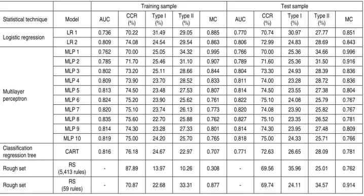
3.1. Testing the relevance of non-financial variables. Table 5 summarizes the results, in terms of AUC, test accuracy, type I-Type II errors, and MC of
all models tested on both the training and test samples. By focusing on the two parametric models (LR 1 and LR 2), our findings show that the AUC of the model which includes the non-financial variables (LR 2) is 80.6%, higher than that which only contains financial ratios as predictor variables (77.0%). Similar results are obtained when the expected misclassification costs14 are analyzed. In this case, our results demonstrate that the combined use of financial and non-financial variables (LR 2) reduces MC by 0.8% (= 0.851 – 0.843) in comparison with using only financial ratios (LR 1). Therefore, in line with other authors (Whittred and Zimmer, 1984; Peel et al., 1986; Altman et al., 2010), we suggest that non-financial information adds value to the model with an improvement of over 3.5% in terms of the AUC and a reduction of 0.8% of the MC. These results confirm our theoretical presumption which states that it seems reasonable to assume that an adequate bankruptcy model made specifically for MEs should not be based solely upon financial ratios, and that non-financial and macroeconomic variables should play a high role. The scarcity, and often misleading nature of financial ratios available for MEs, now amplified by the newly required financial reporting regime in the 2012/06/EU Directive could lie behind the low predictive power that financial ratios have in ME failure prediction. Accordingly, we encourage the collection of non-financial information as early warning variables. Table 5. AUC, correct classification rate, type I-II errors, and misclassification costs 1
Training sample Test sample
Statistical technique Model AUC CCR
(%) Type I (%) Type II (%) MC AUC CCR (%) Type I (%) Type II (%) MC Logistic regression LR 1 0.736 70.22 31.49 29.05 0.885 0.770 70.74 30.97 27.77 0.851 LR 2 0.809 74.08 24.54 29.54 0.863 0.806 72.99 24.83 28.69 0.843 Multilayer perceptron MLP 1 0.762 70.00 25.05 34.32 0.995 0.766 70.00 25.36 34.66 0.996 MLP 2 0.785 71.70 25.46 31.10 0.907 0.789 71.60 25.36 31.50 0.916 MLP 3 0.802 73.20 25.11 28.66 0.844 0.804 73.30 24.93 28.39 0.836 MLP 4 0.809 73.90 23.70 28.52 0.833 0.811 74.00 23.28 28.72 0.836 MLP 5 0.813 74.50 23.48 27.53 0.807 0.814 74.50 23.55 27.38 0.804 MLP 6 0.824 75.20 23.90 25.62 0.761 0.822 75.10 24.08 25.79 0.767 MLP 7 0.820 75.10 23.74 26.13 0.773 0.820 74.08 23.90 25.82 0.767 MLP 8 0.835 75.60 22.70 25.88 0.762 0.827 75.10 23.35 26.52 0.781 MLP 9 0.814 74.30 23.28 27.33 0.801 0.814 74.30 23.95 27.48 0.809 MLP 10 0.819 75.00 24.20 25.70 0.765 0.818 75.00 24.33 25.71 0.766 Classification
regression tree CART 0.816 76.18 24.67 22.97 0.707 0.771 72.63 26.65 28.09 0.781
Rough set RS
(5,413 rules) - 87.89 13.97 10.26 0.308 - 69.56 35.96 25.01 0.762
Rough set RS
(59 rules) - 70.87 22.68 33.31 0.877 - 69.74 24.11 34.57 0.914
1In this study, the values selected for the calculation of the misclassification costs are the following: C
21 = 1 and C12 = 5 recommended by West
(2000); P21 and P12 are dependent on each model; π1 = 0.4898 in the case of the training sample, and 0.5475 for the test sample; and π2 = 0.5102 in
3.2. Comparison of performance of statistical techniques. As can be observed in Table 5 above, in general, the hybrid models fitted in this study – with the exception of the MLP-based models applied with the traditional gradient descent algorithm (MLPs 1, 2, and 3) – outperform traditional LR in terms of the different performance criteria employed. For this reason, second-order training algorithms were also used here (MLPs 7, 8, 9, and 10). These training rules allow for an increase in the AUC values and for a decrease in the misclassification costs, thereby significantly reducing the time spent in training. The MLP model that yields the highest AUC values (0.827 in the test sample) uses the Levenberg-Marquardt training algorithm (MLP 8), which has fourteen hidden nodes and whose sum squared error (SSE) is 0.165. However, considering the misclassification costs, the best MLP model is that which employs the resilient back-propagation as its learning rule (MLP 10), obtaining an MC of 0.766 in the test sample. From the application of the CART algorithm, as in all hybrid failure models in this study, only the ten variables considered in the LR 2 Model were included as predictors. The best tree contains twenty-eight nodes, and validation and replacement costs of 0.54868 (+/- 0.00587) and 0.47748, respectively (see Figure 1). In the training sample, CART obtained an average correct classification rate (CCR) of 76.18%, and type I-II errors of 24.67% and 22.97%, respectively. The AUC is 0.816. In the test sample, the CCR is 72.63%, the type I-II errors are 26.65% and 28.09%, respectively, and the AUC is equal to 0.771. Based on these results, we suggest that the hybrid model LR-CART obtainssimilar accuracy power, in terms of different performance measures, when compared to the LR approach alone, with the exception of the misclassification costs measure under which the hybrid model clearly outperforms the LR. The main advantage of the LR-CART model is that it offers a clear, visual interpretation of the results despite the fact that it provides a non-linear combination of input variables. In addition, the software employed to build this model determines the relative relevance of each variable within the construction of the tree, and in this way, determines the early warning variables on which firms must act to prevent bankruptcy. Our model provides the following ranking: Rpta (100.00%), Celt (94.14%), Cashta (79.64%), Late_Filing_Days (47.68%), Number_ccjs (38.48%), Industry_Solvency (31.65%), Tdta (27.96%), Ln_Asset (16.20%), Ln_Age (1.31%), and Family_Firm (0.85%).
Finally, the last two rows of Table 5 show the performance obtained by the two hybrid failure models employed in this paper using the LR-RS
approach. The results reveal that, under CCR and MC criteria, the accuracy of the hybrid LR-RS model is even lower than that obtained by the parametric LR. Just in terms of MC the LR-RS model employing 5,413 rules outperforms the LR approach. However, the performance and usefulness of this hybrid model is limited, since a high number of rules generate an impractical inefficient model.Conversely, for the 59-rule LR-RS model, it is possible to establish the relevance of each input predictor by taking into account the number of times that each of the ten variables is in a rule, alone or linked with others. Under this procedure, the most relevant variables to classify non-failed MEs are: Late_Filing_Days with the highest weight (55.5% presence in the rules for no failure) and then Cetl (38.89%). In the case of failed MEs, Ln_Asset is the variable with the highest percentage of presence 56.52%, following Tdta (52.17%). Cashta only appears in two of these rules.
Therefore, from a statistical view, our findings support the development of hybrid bankruptcy models. Their higher accuracy performance, improved interpretability as a result of the parametric method’s inclusion of only the most relevant input variables, and the acceleration of the convergence rate of non-parametric statistical techniques, clearly justify the implementation of these hybrid models to predict ME failure. Particularly relevant is the possibility that the development of hybrid models offers in discerning the variables that explain ME failure. Hybrid methods allow us to somehow open the black-box that characterizes non-parametric methods, and distinguish the early warning variables that influence ME bankruptcy. This previous knowledge allows us to anticipate and take the appropriate steps to improve businesses’ financial positions.
3.3. Economic implications. The results of this paper have relevant economic implications for lenders, MEs, and bank supervisors, among others. For lenders, it represents a reduction in asymmetric information in their dealings with MEs. Furthermore, lenders may more effectively control the credit risk specifically supported by MEs (one of their more numerous customers); calculate their capital requirements in a more risk-sensitive way (Internal Rating Based approach); and apply pricing strategies (interest-rate discrimination) for each ME. From the point of view of MEs, the bankruptcy models provide crucial information about the financial health of a firm to investors, managers and auditors, and present a highly useful aid when making a decision to invest, detecting internal problems, and grading the company in terms of (in)solvency risk. For bank supervisors, the
application of a ‘mixed’ failure model is a source of support which includes financial and non-financial variables to determine regulatory capital requirements.
From a methodological perspective, our findings support the development of bankruptcy models using non-financial and macroeconomic variables, and hybrid statistical methods. First, the value added by non-financial and macroeconomic information is substantial given the paucity of publicly available financial data for MEs under the new financial reporting regimen laid down in the recent 2012/06/EU Directive. Second, our hybrid failure models better distinguish the input variables that predict bankruptcy, opening the black-box that characterizes non-parametric statistical techniques. Lastly, it is worth noting that the failure models developed here are, to the best of the authors’ knowledge, the first models fully adapted to publicly available financial ratios under the new ME accounting norms, as established in the 2012/6/EU Directive.
Conclusion
This study compares different hybrid failure models made specifically for MEs, on the premise that the selection of input variables made by the LR model, first, followed by the classification provided by alternative non-parametric methods (MLP, RS, and CART), combined offer better accuracy performance and interpretability than the implementation in isolation of each one of these statistical approaches. In addition, convergence is accelerated.
Our findings show relevant conclusions. First, in general, the hybrid models predict ME failure, obtaining higher accuracy performance in terms of the AUC, test accuracy and Type I-II errors and lower misclassification costs than the traditional LR approach alone. Therefore, hybrid bankruptcy prediction models, especially those developed under the LR-MLP paradigm, constitute relevant tools that enable all users: (1) to make better decisions, by reducing the uncertainty associated with decision making and, thus, reducing the costs associated with poor business decisions; (2) to obtain parsimonious failure models, improving the interpretability of the resulting models; and, (3) to reduce the dimension and to accelerate the convergence rate of non-parametric techniques. In this way, the advantages of both statistical approaches can be harnessed, by first ,implementing LR and, then, a non-parametric model to provide effective synergies between them. Secondly, the hybrid bankruptcy model built on LR-MLP approaches outperforms the other alternative
hybrid methods implemented in this study, LR-RS and LR-CART. The results show that precisely the proposed MLP-based failure model achieves high accuracy, superior by 2.47% to those obtained by LR-CART and 5.54% and 5.36% to those provided by LR-RS, in terms of CCR. Similarly, the comparison in terms of MC also suggests that the LR-MLP generates substantial savings in costs when compared to LR-CART (1.5%) and LR-RS (14.8%). Therefore, based on these findings, we recommend the use of the MLP as a non-parametric statistical method to predict the failure of MEs to the detriment of CART and RS, despite the advantage of transparency that RS and CART have over the MLP by avoiding the black-box feeling of the latter. As affirmed by West (2000), just a mere 1% improvement in accuracy would reduce losses in a large loan portfolio and save millions of dollars. Third, our results demonstrate that the non-financial and macroeconomic variables can complement financial ratios for the prediction of ME failure. Therefore, we suggest the combined use of financial, non-financial and macroeconomic variables, since together they increase the AUC and considerably decrease MC. Quantitatively, we find that the improvement, in terms of the AUC, thanks to the introduction of non-financial and macroeconomic predictors, is 3.6%; even higher than the improvement that involves the use of the best hybrid failure model, LR-MLP (2.1%). However, the LR-MLP model significantly decreases the MC (7.7%). Therefore, we conclude that the predictive power added by non-financial and macroeconomic information is very relevant in the case of MEs, even more so in a new regulatory environment which limits the financial ratios available for these types of firms with the enactment of Directive 2012/6/EU.
All ME stakeholders, particularly banks, creditors and shareholders, should carefully consider the results of this research for the detection of financial distress. In this regard, in a restrictive environment such as the one presented here, where viable investment projects planned by small firms cannot be carried out by weak and cautious financial intermediaries, our bankruptcy model provides an innovative paradigm not only for the mitigation of the risk of a default occurring in the micro-entity segment, but also for the improvement in access to funding resources (mainly in the form of equity, bank debt, and commercial debt) by this type of firm. Additionally, the models developed here are useful for ME managers to analyze internal problems and control the performance of the company, by anticipating insolvency situations and working towards their solution.
This study can be further improved by (a) comparing other non-parametric methodologies such as support vector machines and (b) collecting
non-financial information of a potentially relevant nature in an effort to increase the default prediction accuracy of our models.
References
1. Angelini E., di Tollo G., Roli, A. (2008). A neural network approach for credit risk evaluation, Q. Review of
Economics & Finance, 48(4), pp. 733-755.
2. Altman E.I., Sabato, G. (2007). Modeling credit risk for SMEs: Evidence from US market, Journal of Accounting,
Finance & Business Studies, 43(3), pp. 332-357.
3. Altman, E.I., Sabato, G., Wilson, N. (2010). The Value of Non-Financial Information in Small and Medium-Sized Enterprise Risk Management, Journal of Credit Risk, 6(2), pp. 95-127.
4. Berger A.N., Frame, S.W. (2007). Small business credit scoring and credit availability, Journal of Small Business
Management, 45(1), pp. 5-22.
5. Beyer, A., Cohen, D., Lys, T., Walther, B. (2010). The financial reporting environment: Review of the recentliterature, Journal of Accounting & Economics, 50 (2-3), pp. 266-343.
6. BIS, Department for Business, Innovations and Skills. Simpler financial reporting for micro-entities: The UK’sproposal to implement the ‘micros directive’,https://www.gov.uk/government/uploads/system/uploads/ 7. attachment_data/file/86259/13-626-simpler-financial-reporting-for-micro-entities-consultation.pdf. Accessed on24
September 2014.
8. Bishop, C.M. (1995). Neural networks for pattern recognition. New York, Oxford UniversityPress.
9. Breiman, L. (1988). Submodel selection and evaluation in regression: The x-fixed case and little bootstrap.Technical Report No. 169, Statistics Department, U.C. Berkeley.
10. Breiman, L., Friedman, J., Olshen, R., Stone, C. (1984). Classification and regression trees. Wadsworth, Belmont, CA. 11. Castro, A., Carballo, R., Iglesias, G., Rabuñal, J.R. (2014). Performance of artificial neural networks in nearshorewave
power prediction, Applied of Soft Computing, 23, pp. 194-201.
12. Carter, R., Van Auken, H. (2006). Small firm bankruptcy, Journal of Small Business Management, 44(4), pp. 493-512. 13. Chan, C.C. (2004). Learning rules from very large databases using rough multisets. In J. Peters, A. Skowron,
J.W.Grzymala-Busse, B. Kostek, R.W. Swiniarski, M. Szczuka (eds.). LNCS Transactions on Rough Sets, pp. 59-77, Springer -Verlag Berlin Heidelberg.
14. Chen, M.Y. (2011). Predicting corporate financial distress based on integration of decision tree classification andlogistic regression, Expert Systems with Applications, 38, pp. 11261-11272.
15. Chen, S., Härdle, W.K., Moro, R.A. (2011). Modeling default risk with support vector machines, Quantitative
Finance, 11(1), pp. 135-154.
16. Ciampi, F., Gordini, N. (2013). Small enterprise default prediction modeling through artificial neural networks: Anempirical analysis of Italian small enterprises, Journal of Small Business Management, 51(1), pp. 23-45. 17. Claessens, S., Djankov, S., Lang, L.H. (2000). The separation of ownership and control in East Asian corporations,
Journal of Financial Economics, 58, pp. 81-112.
18. Collis, J. (2012). Determinants of voluntary audit and voluntary full accounts in micro- and non-micro small companies in the UK, Accounting & Business Research, 42(4), pp. 441-468.
19. Crone, S.F., Finlay, S. (2012). Instance sampling in credit scoring: An empirical study of sample size andbalancing, International Journal of Forecasting, 28(1), pp. 224-238.
20. Dedman, E., Kausar, A. (2012). The impact of voluntary audit on credit ratings: Evidence from UK private firms,
Accounting & Business Research, 42(4), pp. 397-418.
21. Dietsch, M., Petey, J. (2004). Should SME exposures be treated as retail or corporate exposures? A comparative analysis of default probabilities and asset correlation in French and German SMEs, Journal of Banking & Finance, 28(4), pp. 773-788.
22. Dimitras, A.I., Slowinski, R., Sumaga, R., Zopounidis, C. (1999). Business failure prediction using rough sets,
European Journal of Operational Research, 114(2), pp. 263-280.
23. Directive 2012/6/EU: Directive 2012/6/EU of the European Parliament and of the Council of 14 March 2012.
http://eur-lex.europa.eu/LexUriServ/LexUriServ.do?uri=OJ:L:2012:081:0003:0006:en:PDF (2012). Accessed on
24 September 2014.
24. Eisenbeis, R. (1977). Pitfalls in the application of discriminant analysis in business, finance, and economics,
Journal of Finance, 32(3), pp. 875-900.
25. Engelmann, B., Hayden, L.E., Tasche, D. (2003). Testing rating accuracy, Risk, 16, pp. 82-86.
26. Fan, C.Y., Pei-Chann, C., Jyun-Jie Lin, L., Hsieh, J.C. (2011). A hybrid model combining case-based reasoningand fuzzy decision tree for medical data classification, Appl. Soft Computing, 11(1), pp. 632-644.
27. Gibbons, J.D., Chakraborti, S. (2014). Nonparametric statistical inference, International Encyclopedia Statistical Science, pp. 977-979.
28. Gepp, A., Kuldeep, K., Bhattacharya, S. (2009). Business failure prediction using decision trees, Journal of
Forecasting, 6, pp. 536-555.
29. Grunert, J., Norden, L., Weber, M. (2005). The role of non-financial factors in internal credit ratings, Journal of
Banking & Finance, 29(2), pp. 509-531.
30. Hastie, T., Tibshirani, R., Friedman, J.H. (2009). The elements of statistical learning: Data mining, inference,
31. Jagric, V., Kracun, D., Jagric, T. (2011). Does non-linearity matter in retail credit risk modeling? Czech Journal of
Economics & Finance, 61(4), pp. 384-402.
32. Jones, F.L. (1987). Current techniques in bankruptcy prediction, Journal of Accounting Literature, 6, 131-164. 33. Karels, G., Prakash, A. (1987). Multivariate normality and forecasting of business bankruptcy, Journal of
Business, Finance and Accounting, 14(4), pp. 573-593.
34. Kim, K.J. (2003). Financial time series forecasting using support vector machines, Neurocomputing, 55, pp. 307-319. 35. Marquez, L., Hill, T., Worthley, R., Remus, W. (1991). Neural network models as an alternative to regression. 36. Proceedings of the IEEE 24th Annual Hawaii International Conference on Systems Sciences 4, pp. 129-135. 37. Moon, T., Sohn, S. (2010). Technology credit scoring model considering both SME characteristics and economic
conditions: The Korean case, Journal of the Operational Research Society, 61(4), pp. 666-675.
38. Peters, A., Hothorn, T. (2012). ipred: Improved Predictors. R package version 0.8-13. Available at:
http://CRAN.R-project.org/package=ipred.
39. Neves, J.C., Vieira, A. (2006). Improving bankruptcy prediction with hidden layer learning vector quantization,
European Accounting Review, 15(2), pp. 253-271.
40. Nguyen, S.H., Skowron, A., Synak, P., Wróblewski, J. (1997). Proc. of The Seventh International Fuzzy Systems Association World Congress, 2, pp. 204-209.
41. Olson, D.L., Denle, D., Meng, Y. (2012). A comparative analysis of data mining methods for bankruptcyprediction, Decision Support Systems, 52, pp. 464-473.
42. Pawlak, Z. (1991). Rough sets: Theoretical aspects of reasoning about data. Kluwer Academic Publishers. 43. Peel, M.J., Peel, D.A., Pope, P.F. (1986). Predicting corporate failure – Some results for the UK corporate sector,
Omega International Journal of Management Science, 14(1), pp. 5-12.
44. RaviKumar, P., Ravi, V. (2007). Bankruptcy prediction in banks and firms via statistical and intelligenttechniques – A review, European Journal of Operational Research, 180(1), pp. 1-28.
45. Rodrigues, B.D., Stevenson, M.J. (2013). Takeover prediction using forecast combinations, International Journal
Forecasting, 29(4), pp. 628-641.
46. Rumelhart, D.E., Hinton, D.E., Williams, R.J. (1986). Learning internal representations by error propagation
inparallel distributed processing. Cambridge, MA: MIT Press (1986).
47. Sánchez-Lasheras, F., de Andrés, J., Lorca, P., de Cos Juez, F.J. (2012). A hybrid device for the solution of sampling bias problems in the forecasting of firms´bankruptcy, Expert Systems with Applications, 39(8), pp. 7512-7523.
48. Slowinski, R., Zopounidis, C. (1995). Application of the rough set approach to evaluation of bankruptcy risk,
International Journal of Intelligent Systems in Accounting, Finance & Management, 4(1), pp. 27-41.
49. Timmermann, A. (2006). Forecast combinations. In: G. Elliott, C. Granger, & A. Timmermann (eds.), Handbook
of economic forecasting. Elsevier.
50. Venables, W.N., Ripley, B.D. (2002). Modern applied statistics with S-PLUS. New York: Springer.
51. West, D. (2000). Neural network credit scoring models, Computers & Operations Research, 27, (11/12), pp. 1131-1152.
52. Whittred, G.P., Zimmer, I. (1984). Timeliness of financial reporting and financial distress, Accounting Review, 59(2), pp. 297-295.
53. Wilson, N., Altanlar, A. (2013). Company failure prediction with limited information: Newly incorporatedcompanies,
Journal of the Operational Research Society. 1, pp. 1-13.
54. Wilson, N., Wright, M., Scholes, L. (2013). Family business survival and the role of boards, Entrepreneurship
Theory & Practice, 37(6), pp. 1369-1389.
55. Witten, I.H., Frank, E. (2005). Data mining, practical machine learning tools and techniques. San Francisco: Morgan Kaufmann.
56. Wong, F.S. (1991). Time series forecasting using backpropagation neural networks, Neurocomputing, 2, pp. 147-159. 57. Zhang, G.P., Patuwo, B.E., Hu, M.Y. (1998). Forecasting with artificial neural networks: The state of the art,
International Journal of Forecasting, 14(1), pp. 35-62.
Appendix 1
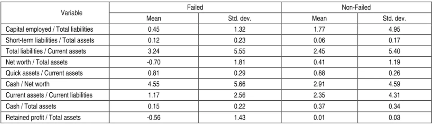
Table A.1. Descriptive statistics of the quantitative predictor variables
Variable Failed Non-Failed
Mean Std. dev. Mean Std. dev.
Capital employed / Total liabilities 0.45 1.32 1.77 4.95
Short-term liabilities / Total assets 0.12 0.23 0.06 0.17
Total liabilities / Current assets 3.24 5.55 2.45 5.40
Net worth / Total assets -0.70 1.81 0.41 1.19
Quick assets / Current assets 0.81 0.29 0.88 0.26
Cash / Net worth 4.55 5.66 2.91 4.59
Current assets / Current liabilities 1.17 2.56 2.35 4.31
Cash / Total assets 0.15 0.22 0.37 0.34
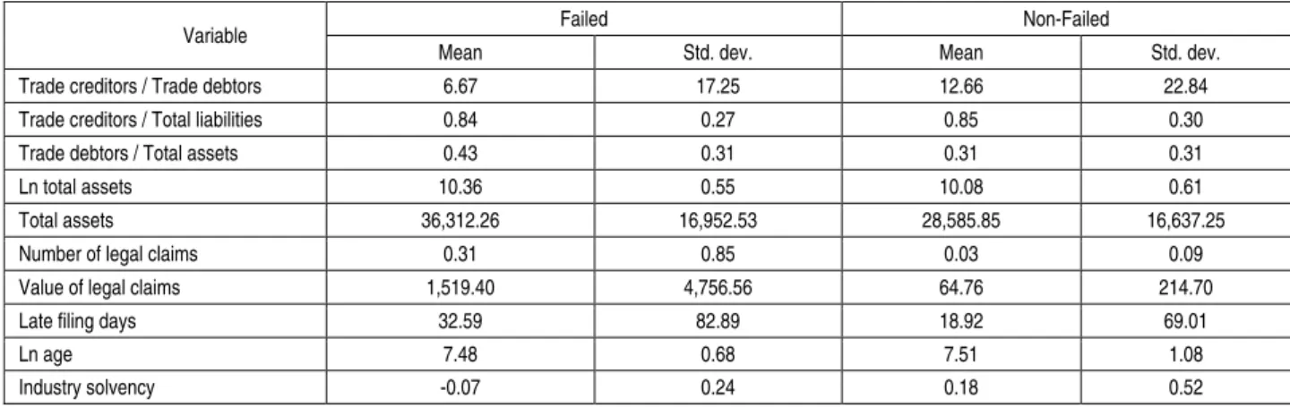
Table A.1 (cont.). Descriptive statistics of the quantitative predictor variables
Variable Failed Non-Failed
Mean Std. dev. Mean Std. dev.
Trade creditors / Trade debtors 6.67 17.25 12.66 22.84
Trade creditors / Total liabilities 0.84 0.27 0.85 0.30
Trade debtors / Total assets 0.43 0.31 0.31 0.31
Ln total assets 10.36 0.55 10.08 0.61
Total assets 36,312.26 16,952.53 28,585.85 16,637.25
Number of legal claims 0.31 0.85 0.03 0.09
Value of legal claims 1,519.40 4,756.56 64.76 214.70
Late filing days 32.59 82.89 18.92 69.01
Ln age 7.48 0.68 7.51 1.08
Industry solvency -0.07 0.24 0.18 0.52
Table A.2. Descriptive statistics of the qualitative predictor variables
Variable Category Status Frequency (%)
Charge on asset No (0) Failed 46.75 Non-Failed 49.40 Yes (1) Failed 3.25 Non-Failed 0.60 Family firm No (0) Failed 28.30 Non-Failed 25.56 Yes (1) Failed 21.70 Non-Failed 24.44 Audited accounts No (0) Failed 47.26 Non-Failed 48.14 Yes (1) Failed 2.74 Non-Failed 1.86
Positive judgment audit report
No (0) Failed 48.10 Non-Failed 48.32 Yes (1) Failed 1.90 Non-Failed 1.68 Change auditor No (0) Failed 47.40 Non-Failed 47.63 Yes (1) Failed 2.60 Non-Failed 2.37
Table A.3. Definition and explanation of the non-financial predictor variables
Variable Definition
Number/Value of legal claims
Both variables are related with financial distress situation since, on the majority of occasions, previous to declaring themselves bankrupt, the companies tend to present defaults in some of their payments. If this delay is prolonged in time, suppliers often bring a legal claim to collect the money owed to them. Therefore, the accumulation of legal claims (LCs) against a company is indicative that this firm is financially troubled, which can lead to the failure of the company. We use both: (i) the number of LCs (Number_LCs) against a company and, (ii) the value, in monetary units, of these LCs (Value_LCs).
Late filing days
In the U.K., firms have 10 months to submit their annual accounts. The late submission of annual accounts is a violation of business regulations and is usually due to reasons that adversely affect the company's financial health. Late submission is likely to be an indicator of financial distress.
Charge on asset
In the case of borrowers of higher credit risk, lenders often require financing to be secured by charges on assets of the company. Consequently, we assume that the borrowers who have charges on assets will have a higher probability of bankruptcy than those who do not. For this reason, we consider that firms with charges on assets hoard higher risk of bankruptcy.
Family firm Family firms often have certain problems linked to their own idiosyncrasies, such as family successions, non-professional CEOs and low productivity. Therefore, we posit that family companies run a greater likelihood of failure than non-family firms.
Audited accounts This variable states whether the annual accounts of a micro-entity is, or not, audited. Audited accounts, takes a value of 1 where the firm has been audited, and 0 otherwise.
Positive/Negative judgment audit report
The audit report issued by the auditors can highlight financial problems in the firms which are often linked to bankruptcy situations. Auditors can qualify accounts according to the severity of their concerns.
Change auditor
Frequently, the change in the auditor is linked to discrepancies of criteria between the auditor and firm about the contents of the audit report. These discrepancies often happen when the auditor highlights problems which adversely affect the financial health of the company.