Predicting financial distress through machine learning

(1)

FACULTAT D’INFORMÀTICA DE BARCELONA MASTER ININNOVATION ANDRESEARCH ININFORMATICS

DATAMINING ANDBUSINESSINTELLIGENCE

M

ASTER

T

HESIS

Predicting Financial Distress Through

Machine Learning

Author:

Malika IBRAIMOVA

Supervisor: Alfredo VELLIDO

A thesis submitted in fulfillment of the requirements for the degree of Master in Innovation and Research in Informatics

Computer Science Department

(2)

(3)

iii

Declaration of Authorship

I, Malika IBRAIMOVA, declare that this thesis titled, “Predicting Financial Distress Through Machine Learning” and the work presented in it are my own. I confirm that:

• This work was done wholly or mainly while in candidature for a research de-gree at this University.

• Where any part of this thesis has previously been submitted for a degree or any other qualification at this University or any other institution, this has been clearly stated.

• Where I have consulted the published work of others, this is always clearly attributed.

• Where I have quoted from the work of others, the source is always given. With the exception of such quotations, this thesis is entirely my own work.

• I have acknowledged all main sources of help.

• Where the thesis is based on work done by myself jointly with others, I have made clear exactly what was done by others and what I have contributed my-self.

Signed: Date:

(4)

(5)

v

Abstract

The beforehand identification of future financial distress of a company might be very helpful for managers, stockholders, creditors and other interested third parties to discover the financial health of company more deeply. The main question which will be raised in this thesis is - whether we can predict future financial distress of a company based on the changes in historical financial results using different ma-chine learning techniques. The predictions were made based on changes in financial results during three different time intervals, which are: one year, half-year and a quarter before expected bankruptcy. The financial data of banks used in analysis was obtained from the quarterly reports presented on the website of the Federal Deposit Insurance Corporation. The results of analysis indicated that classification model developed by RBF kernel SVM using the data, obtained from PCA analysis on the basis of quarterly changes of the financial data, best predicts future financial distress in banks of Unites States of America.

(6)

(7)

vii

Acknowledgements

I would like to thank my supervisor, Alfredo Vellido, for his assistance and guidance which facilitated my work. A special thanks to my family for providing me with endless support throughout my university studies. . . .

(8)

(9)

ix

List of Figures

2.1 Conceptual overview of Exploratory Factor Analysis . . . 8

2.2 An orthogonal projection process in PCA . . . 10

2.3 Scree test of eigenvalues . . . 12

2.4 The KNN approach . . . 14

2.5 Architecture of the Self-Organizing Map . . . 16

2.6 Architecture of the Supervised SOM for classification problem . . . 18

3.1 Number of banks which faced financial distress during the 1992-2017 period in the U.S. . . 21

3.2 Total number of banks in U.S. during 1992-2017 . . . 22

3.3 Loans and Leases group’s boxplots: Scenario 1 . . . 24

3.4 Loans and Leasesgroup density plots: Scenario 1 . . . 24

3.5 Total Depositsgroup boxplots: Scenario 2 . . . 25

3.6 Total Depositsgroup density plots: Scenario 2 . . . 25

3.7 Performance and Condition Ratiosgroup boxplots: Scenario 3 . . . 26

3.8 Performance and Condition Ratiosgroup density plots: Scenario 3 . . . . 26

3.9 Scree plot: Scenario 1 . . . 27

3.10 The first 3 dimensions obtained from PCA: Scenario 1.. . . 28

3.15 Very Simple Structure Fit . . . 31

3.16 Exploratory Factor Analysis: Scenario 1 (1 Part) . . . 33

4.1 Importance of variables in KNN models obtained from EFA. . . 44

4.2 Importance of variables in RF models obtained from EFA.. . . 46

4.3 Importance of variables in Gaussian kernel SVM models obtained from EFA.. . . 47

4.4 Importance of variables in RBF kernel SVM models obtained from EFA. 48 4.5 Importance of variables in 2-degree Polynomial kernel SVM models obtained from EFA. . . 50

4.6 Importance of variables in 3-degree Polynomial kernel SVM models obtained from EFA. . . 51

4.7 Importance of variables in supervised SOM models obtained from EFA. 53 4.8 Supervised SOM models. . . 55

(12)

(13)

xiii

List of Tables

3.1 Groups of exploratory variables. . . 23

4.1 KNN results . . . 45

4.2 Random Forests results . . . 46

4.3 SVM results . . . 52

(14)

(15)

xv

List of Abbreviations

CFA ConfirmatoryFactorAnalysis EFA ExploratoryFactorAnalysis FA FactorAnalysis

FDIC FederalDepositInsuranceCorporation ICA IndependentComponentAnalysis KMO KaiserMeyerOlkin

KNN K-NearestNeighbors ML MaximumLikelihood PC PrincipalComponent

PCA PrincipalComponentAnalysis RF RandomForests

SOM Self -OrganizingMaps SVM SupportVectorMachines U.S. UnitedStates of America VIF VarianceInflationFactors VSS VerySimpleStructure

(16)

(17)

1

Chapter 1

Introduction

1.1 Motivation

Bankruptcy is a process that a legal entity or an individual undertakes in order to protect or liquidate assets to repay debts, depending on the situation. Judging by the financial crisis history and multiple valuations of the several banks’ behaviors -bankruptcy is not a problem as such, but a measure taken to solve a bigger problem. Many myths surrounding bankruptcy often create a barrier in the human mind to adequately assess the financial situation of the legal entity. When foreseen before-hand, the bankruptcy can actually become a great tool to avoid further damage and total annihilation of personal assets. That is why it is extremely important to be able to predict any possible financial distress in a company and have up-to-date and con-stantly improving algorithms that will help to analyze the future financial health of an organization through the financial dynamics of the organization.

Financial distress of the legal entity can be caused by numerous factors that are extremely important to be observed. In today’s world, every legal entity has to con-sider the preemptive measures that will help either to foresee the financial distress and try to avoid it, or file for bankruptcy at the right time. Let us bring about the case of the Lehman Brothers investment bank going bankrupt in September of 2008, an institution that was established in 1850. The financial crisis itself did not begin because of Lehman Brothers having to go bankrupt. The financial crisis had been lurking for the more than a year before this bankruptcy came to happen. A large US investment bank, Bear Stearns, had to be saved in March of 2007. The systematic loss of trust amongst financial institutions towards each other’s solvency caused the stress. United States Bankers had made huge benefits by selling “risk free” assets, called mortgage-backed securities, which were basically subprime mortgages mixed together with a better-quality mortgage. In 2006, the Central Bank of The United States had raised the interest which made many households to go default, leading to a decrease in house prices, making it clear that mortgage-backed securities were very risky. Risky securities were owned by almost every bank and it was impossible to recognize which bank was more strongly damaged by the bad debts. Because of all the distrust among each other, banks started to charge high rates to other banks that were suspicious to have unrecognized damage from the mortgage backed secu-rities. And it was precisely in this period of distrust when banks stopped to lend to each other that Lehman Brothers went bust1.

Why did such a huge investment bank had to file for bankruptcy? The answer is a failure to properly predict the financial distress that was about to hit the U.S. econ-omy and subsequently holding on to the problematic assets and low-rated mort-gages that amounted to the figure 30 times bigger than its capital. However, there are

1 https://www.independent.co.uk/news/business/analysis-and-features/financial-crisis-2008-why-lehman-brothers-what-happened-10-years-anniversary-a8531581.html

(18)

also cases of a timely financial distress prediction that helped the banks to avoid un-necessary damages. The BNP Paribas bank, formerly controlled by the government and with current headquarters in Paris, France, is the third largest bank in European Union. The BNP Paribas bank was able to avoid the financial distress of 2007-2008 because of its more conservative business structure and forecasting. More than a half of the BNP Paribas’s revenue came from retail banking in European Countries like France, Spain and Italy. Due to their substantial accumulated retail deposits that were $659 billion in 2007, BNP Paribas were able to avoid short-term lending and fund its investment banking operations with existing capital2.

Predicting financial distress is an activity aimed at identifying and studying pos-sible dangers for the future development of a company. For sustainable develop-ment, each company must make predictions about its future financial condition. This is due to the fact that predicting financial distress for a company is of great importance, since it helps to reduce various types of risks that affect the financial condition, increase the efficiency of the company, increase profitability and help to avoid bankruptcy of the company. Financial condition prediction is characterized by uncertainty, which is a problem, since for forecasting it is necessary to take into account many factors that may affect the company in the future. However, after an-alyzing the most likely factors that may have influence on the financial health of the company, the company’s future financial condition can be predicted and the threats that may lead to a decrease in financial viability or even bankruptcy can be foreseen.

1.2 Goals and Research Questions

The research in this thesis is aimed at building a model which can accurately predict future financial distress of a company. The main goal leads in turn to several sub-goals which will be described in this section.

Most of the research in the field of bankruptcy prediction has been carried out using the financial ratios of the company as the exploratory variables. In case of this study, availability of U.S. banks’ financial data allowed us to increase the number of factors that may affect the future financial condition of the company. Also, previous work examined in their analysis only the financial results of the firm for the specific period before the predicted bankruptcy date. The novelty of this study is that it tries to find out if the changes in financial data during a specific period before expected bankruptcy can properly predict it. So, the first question raised in this study can be formally stated as:

• Q1: How relevant are the changes in historical financial data for bankruptcy predic-tion?

The number of features used in the analysis is quite significant. So, there is a need for dimensionality reduction and feature extraction in order to make the inter-pretation of the results amenable. In order to do it, two different techniques were implemented, namely: Principal Component Analysis (PCA) and Factor Analysis (FA). This leads to the second question:

• Q2: Which dimensionality reduction and feature extraction technique is more useful in the analysis and, can we extract hidden information from the new features?

2_{http://archive.fortune.com/2008/08/27/news/companies/demos}

(19)

1.3. Outline 3 The prediction accuracy varies depending on the technique used to build the model. Obtaining the best prediction accuracy is the main goal. So, different su-pervised machine learning techniques, namely, Support Vector Machines (SVM), K-Nearest Neighbors (KNN), Random Forests and Supervised Self-Organizing Maps (XY-Fused networks) were compared to answer the following question:

• Q3: Which machine learning technique best predicts the financial distress of a com-pany?

The main objective of the study is not only to predict the bankruptcy of a com-pany based on the changes in financial results, but, also, to identify the historical time interval which best suits for predictions. So, the changes in financial data oc-curred during three different time intervals were considered. Those intervals are: year, half-year and quarter before prediction period. So, third question is stated as:

• Q4: How far in advance can we predict bankruptcy?

All the experiments and background information needed to answer the ques-tions listed above will be disclosed in this thesis.

1.3 Outline

This study is divided into five chapters: introduction, background, materials and methods, classification experiments and conclusion. After this brief introduction, in chapter2, we present the background of this work, including a brief presentation of the banking system of the United States of America; we discuss previous work in this area; and we describe the machine learning algorithms and concepts used in the analyses.

The first part of chapter3describes the data used to build the model and the data pre-processing steps that were conducted, including the dimensionality reduction and feature extraction processes.

The chapter4depicts the machine learning algorithms and their implementation with a focus on the technical side and the results of classification methods used for model development and, finally, the conclusions and some possible extensions of this work are presented in chapter5.

(20)

(21)

5

Chapter 2

Background

This chapter provides an overview of the general information about the banking industry of United States of America and the main machine learning algorithms which were used in this work. Several related works in bankruptcy prediction were reviewed with comparative view of the techniques and approaches proposed by the authors.

2.1 Banking

Banking is an industry that works with the main means of economic exchange in the society. Banks offer different cash transactions, credits and a reliable place to keep savings for their clients, which includes savings accounts, checking accounts and deposits. Using the money that is stored in the deposits, banks can provide different types of loans that include mortgages, cars or business loans. Banking has always been one of the most vital parts of the United States economy, since most of its citizens have long-term liabilities to banks. By providing loans for families and entrepreneurs, banks provide an opportunity for people who do not have big savings to invest into the education, housing or businesses.

Insured by the Federal Deposit Insurance Corporation (FDIC), banks are the most reliable institution to deposit cash. Banks, in their turn, not only provide a safe storage for the cash, but also reward the depositors by a certain interest rate paid to them on monthly or yearly basis. According to FDIC requirements, banks are obliged to keep only 10 percent of their deposits and lend the other 90 percent with higher interest rates than they reward their depositors with. Therefore, it is easy for banks to make money. It is also true that banks should always balance it’s operations in order to prevent financial problems in the future.

2.1.1 The banking system of the United States of America

The banking system of United States of America (U.S.) consists of a few different types of banking institutions, which are: commercial banks, community banks, re-tail banks, credit unions, mutual banks, savings banks, savings and loans, online banks and central banks (The Federal Reserve). Commercial banks provide differ-ent financial services to individuals and to businesses, while retail banking provides its services only to individuals and families. Community banks are smaller than commercial banks and provide fewer financial operations, concentrating on the lo-cal market. Credit unions and mutual banks are owned by individuals which are members of it. These types of institutions provide more personalized services. Sav-ings banks are focused only on providing the saving accounts, while saving and loan institutions provide saving accounts and several types of loans. As can be seen from

(22)

the name, online banks provide all of their services on-line and do not have physical locations.

A chain of events that included financial panic that damaged the U.S. economy in 19th and the beginning of the 20th century led to the creation of the Federal Reserve System or central bank. Among others, the central bank has four major functions, which are1:

• Monetary policy of the U.S., which includes conditions of credit and long term interest rates.

• Ensuring safety of the financial and banking system.

• Overlooking the stability and systemic risks of the financial system.

• Handling the payment system in both domestic and international domains. 2.1.2 Federal Deposit Insurance Corporation

The Federal Deposit Insurance Corporation (FDIC) is an independent agency of the U.S. government that protects the funds that depositors place in banks and savings associations. FDIC insurance is backed by the full faith and credit of the U.S. gov-ernment. Since the FDIC was established in 1933, no depositor has lost a cent of FDIC-insured funds2. FDIC insurance covers all deposit accounts, including:

• Checking accounts • Savings accounts

• Money market deposit accounts • Certificates of deposit

FDIC insurance does not cover other financial products and services that banks may offer, such as stocks, bonds, mutual funds, life insurance policies, annuities or secu-rities. The standard insurance amount is $250,000 per depositor, per insured bank, for each account ownership category3.

2.1.3 Financial data

Financial data reflects the financial condition of a company and should be tied to a specific period of time in the past. It consists of day-to-day bookkeeping infor-mation. The financial data of a company is used in preparation of the company’s financial statements. Financial statements are used by internal and external man-agement to analyze and audit the business performance of the entity. In fact, there are four main types of financial statements:

• Balance sheets • Income statements • Cash flow statements

• Statement of shareholders’ equity 1_{www.federalreserve.gov/faqs/about}

12594.htm 2_{https://www.fdic.gov/about/history/}

(23)

2.2. Dimensionality reduction and feature extraction 7 Balance sheets represent a company’s financial position at the end of a specific time period. Observed periods of time can be a quarter, half year, year, or several years. Balance sheets express the fundamental equation:

Assets=Liabilities+Equity (2.1) Assets represent everything that an entity can own and include all intangible and tangible property. Tangible property is any physical property, whereas intangible property is non-physical, such as a patent or a goodwill.

Liabilities are everything that the company owes to others. Liabilities include such things as debt, accounts payable, wages, benefits, and taxes. Liabilities can be short-term, which means that the they will be due within a year, or long-term if the liabilities should be redeemed within a year or longer.

Stockholders’ equity is known as the book value of a company. It has two main sources: the money initially invested in a firm and additional investments made later. Income statements summarize the total earnings during a period of time. The total earnings are calculated as the difference between total income and expenses. Cash flow statements disclose cash movements during the observed period. State-ments of shareholders’ equity show the changes in the owners’ equity for the certain period.

2.2 Dimensionality reduction and feature extraction

The number of features in an input data vector could easily be as high as tens of thousands. Such a high dimensionality of data could have very adverse effect on data analysis and processing (Kung,2014), this mainly affects the following factors:

• Computational cost. A large dimensionality usually leads to high computa-tional complexity and power consumption both in the (off-line) learning and in the (online) prediction phases. The reduction of the number of dimensions helps to minimize the computation time and might prevent keeping irrelevant features in the data.

• Performance degradation due to sub-optimal search. A high data dimensional-ity may cause the numerical process to converge prematurely to a sub-optimal solution.

• Data visualization. It is connected with humans’ inability to see objects geo-metrically in high-dimensional spaces.

• Data over-fitting. In supervised learning, when the input vector dimension far exceeds the number of training samples, data over-fitting becomes highly likely.

Dimensionality reduction offers an effective remedy to mitigate the above-mentioned problems. This data pre-processing step can also help in reducing the noise in the data, as it is possible to have irrelevant features or high multicollinearity in the data collected.

Next, we will discuss two primary techniques for dimension reduction and fea-ture extraction considered in the thesis, namely Factor Analysis (FA) and Principal Component Analysis (PCA).

(24)

2.2.1 Factor Analysis

Factor analysis is a statistical technique that is widely used in psychology and the social sciences at large. It was originally developed by Spearman in 1904 in the area of human abilities in particular, to answer the question of why human abilities are always positively correlated. Factor analysis is a method for investigating whether variables of interestX1, X2, . . . ,Xn, are linearly represented by a smaller number

of unobservable factorsF1,F2, . . . ,Fk. The variables which make up these factors

should be generally more correlated to each other than the factors are to each other. The orthogonal model underlying FA can be described by Equation 2.2 (Hewson, 2009) :

X =µ+Γα+e, (2.2)

whereXis an 1∗nrandom vector,µrepresents a vector of unknown constants (mean values), Γis an unknownn∗k matrix of constants referred to as the loadings, αis a 1∗kunobserved random vector referred to as the scores assumed to have mean 0, e is 1∗n unobserved random error vector having mean 0 and by assumption a diagonal covariance θ referred to as the uniqueness or specific variance. Factor loadings (Γ) are defined as the correlations between variables and factors.

FA is an ambiguous model, as it is unchanged if we replace Γ by KΓ for any orthogonal matrix K. This is a potential problem, but it can turn into an advan-tage because, with a reasonable choice of a suitable orthogonal matrix K, we can achieve a rotation that may yield a more interpretative result. FA therefore requires an additional stage, having fitted the model we may wish to consider rotation of the coefficients. We must keep in mind that orthogonally rotated factors have zero or negligible intercorrelation by definition. An oblique rotation provides a degree of correlation between factors to improve the mutual correlation between elements within the factors.

FIGURE2.1: Conceptual overview of Exploratory Factor Analysis.

(25)

2.2. Dimensionality reduction and feature extraction 9 • Exploratory factor analysis (EFA): attempts to uncover the nature of the

con-structs, influencing a set of responses.

• Confirmatory factor analysis (CFA): tests whether a specified set of constructs have the predicted effect on the set of responses.

The EFA is used to reduce the amount of data to be used or identify the number and nature of hidden latent factors in the data. The term "exploratory" is not used casually, as EFA does not test a model of factor structure, rather it examines the data set in search for statistically justified factors. It leads to subjectivity, since determin-ing how many factors to select is a subjective and arbitrary process. (Plucker,2003). The steps for performing EFA are as follows:

• Obtain the data

• Calculate correlation matrix

• Choose the number of factors for inclusion • Extract initial set of factors

• Rotate the factors to obtain final solution • Interpret factors structure

• Construct factor scores for further analysis • Derive the new data set

Despite the many benefits, the FA has also some objections, listed below (Kline, 1994):

• Infinity mathematically equivalent solutions.

• The discrepancy of results. FA frequently leads to disagreement as to what are the most important factors in the problem.

• It is difficult to replicate FA. This statement comes from the first objection. 2.2.2 Principal Component Analysis

Principal Component Analysis is a dimensionality reduction technique of the fea-ture extraction family. It is defined as an orthogonal transformation that linearly transforms a set of observations of possibly correlated variables into a set of values of linearly uncorrelated variables called principal components or PCs (Kung,2014). PCA finds a linear projection of data into orthogonal basis system that has the mini-mum redundancy and preserves the maximini-mum variance in the data. The projection process is illustrated in Figure 2.2 with an example of data set of observations xn

wheren = 1, ..,P, wherexnis a variable of dimensionalityD. The goal is to project

the data into a space of dimensionalityM < D, while maximizing the variance of the projected input data (Bishop,2006). In Figure 2.2, PCA seeks a space of lower dimensionality, which is denoted by the magenta line, such that the orthogonal pro-jection of the data points (red dots) into this subspace maximizes the variance of the projected points (green dots). The new coordinates in the eigenvector basis, i.e. the orthogonal projections onto the eigenvectors, are the aforementioned PCs. The first

(26)

FIGURE2.2: An orthogonal projection process in PCA (Bishop,2006).

PC is chosen as a projection direction such that the projections of the data onto it have maximum variance.

PCA is an unsupervised approach, since it involves only a set of input features

X1,X2, . . . ,Xp, and no associated response or targetY. The number of components extracted from PCA is equal to the number of observed variables in the analysis. The first PC identified accounts for most of the variance in the data. The second accounts for the second largest amount of variance in the data and is uncorrelated with the first principal component, and so on. The steps of the PCA procedure are as follows:

• Obtain data

• Standardize the data

• Calculate correlation matrix

• Calculate eigenvalues and eigenvectors of correlation matrix or perform Sin-gular Vector Decomposition.

• Choose components to retain and form feature vectors • Derive the new data set

The PCA model can be summarized by Equation 2.3, where X is a matrix of observed variables,Zis a matrix of scores on components andBis a matrix of eigen-vectors.

X=ZB (2.3)

The component score is a linear combination of observed variables weighted by eigenvectors. The scores of the first PC of a set of features X1, X2, . . . , Xp is the normalized linear combination of the features, which is presented in Equation 2.4 (G. et al.,2013).

Z1= b11X1+b21X2+...+bp1Xp (2.4)

For dimensionality reduction purposes, the components accounting for maximal variance are retained while other components accounting for a trivial amount of variance are ignored. The eigenvalues indicate the amount of variance explained by each PC. Any PC with near-zero eigenvalues should be removed from analysis, as they do not explain a significant amount of variance in the data.

(27)

2.2. Dimensionality reduction and feature extraction 11 2.2.3 Factor Analysis versus Principal Components Analysis

FA and PCA are often confused with each other, it might occur due to the fact that there is one method of performing FA called Principal Component Extraction. These two methods should never be confused. PCA seeks orthogonal projections of the data according the variance maximization in order to achieve dimensionality reduc-tion, and is not intended to find a reasonable interpretation for all the components that are kept. FA, instead, tries to study the covariance (or correlation) relation-ships between many variables and is based on creates unobservable or latent ran-dom quantities called factors (Hewson,2009) and it is, this, a latent variable model. So, PCA observes the relationships between the individual and total (common and error) variances shared between items, while FA observes the relationship between the individual item variances and common variances shared between items. Some-times, in the early stages of an analysis, FA is preferable to PCA, as it allows you to measure the ratio of an item’s unique variance to it’s shared variance, known as its communality.

FA and PCA have two main conditions. Firstly, there must be some relation/connection (correlation) between the variables. In addition, the larger the sample size, especially in relation to the number of variables, the more reliable the resulting factors. The sample size is less important for factor analysis, since the communalities of objects with other objects are high or relatively high. However, PCA or FA should never be performed if the number of variables is greater than the number of observations in the data set.

There are several similarities between the FA and PCA techniques (Klinke, Mi-hoci, and Hardle,2010; Hardle and Simar,2003), including:

• Based on a linear model

• Aim to reduce the number of data features • Can be used on covariance or correlation matrix

• Provide similar results for the resulting PCs and latent factors (without rota-tion).

And at the same time they have differences, as listed below:

• PCA has an importance ranking of the components determined by the eigen-values while in EFA factors are all equal in the analysis and only might be ranked after rotation based on interpretability of factors which is nonobjective. • PCA is based on a well-defined algorithm, whilst the fitting factor analysis model includes many numerical procedures. The non-uniqueness of the factor analysis procedure opens the door for subjective interpretation and, therefore, produces a range of different results.

• PCA optimises the total variance. Since the total variance is the sum of squared distances to the data centre it is obvious that the covariance or correlation struc-ture of the data does not play any role. EFA aims to reproduce the covariance or correlation matrix as well as possible.

(28)

2.2.4 Selection of the number of components or factors to retain

There are several techniques for the identification of the number of dimensions that should be kept for further analysis, and most of them are commonly used both in FA and PCA. Several of these methods will now be discussed further in this section. The first one is the Kaiser-Guttman rule, also referred to as “the Kaiser criterion”, or “the eigenvalues > 1.0 rule”. It proposes dropping factors whose eigenvalues are less than one, since the variance explained by each of these factors is less than the variance explained by a single variable. The Kaiser–Guttman rule is widely used because of its simplicity.

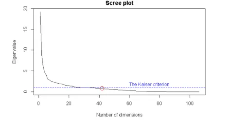
The second approach, called Cattell scree test, is a graph-basedad hoctechnique that uses the eigenvalues that are taken from the input or reduced correlation matrix. As shown in Figure 2.3, the eigenvalues form the vertical axis and the factors form the horizontal axis. The graph is inspected to determine the last substantial decline in the magnitude of the eigenvalues or the point where eigenvalues substantially change slope. This graph is the most popular method for determining the number of factors/dimensions. A limitation of this approach is that the results of the scree test might be ambiguous and open to subjective interpretation (Brown,2006).

FIGURE2.3: Scree test of eigenvalues. Arrow indicates region of the

curve where the slope changes.

Another criterion is to set a certain percentage of variance that needs to be ex-plained, and then keep enough factors/dimensions to achieve this variance from data. Usually, the lower limit is set to be at least 50% of the total variance in the data. The choice of the wright technique among all the above mentioned methods is not straightforward. Perhaps the best advise is to use the number of factors that best agrees with the goals of analysis. If there is no need of substantial dimensionality reduction, it might be better to keep most, if not all, of the factors/dimensions dur-ing the early stages of the analysis. If the goal is to reduce the dimensionality of data, then it is best to keep enough factors/dimensions so that they will explain a reasonably large percentage of the variation in data.

(29)

2.3. Supervised Learning 13

2.3 Supervised Learning

Most machine learning problems can be considered to fall into one of three cate-gories: unsupervised, semi-supervised or supervised. The previous part of this chapter discussed unsupervised methods in this work, and the next part of the thesis is devoted to supervised learning techniques.

The main characteristics of supervised learning models is that for each obser-vation of the predictor measurementxi, i = 1, ...,n there is an associated response

measurementYi, and the goal is fitting a model that relates the response to the

pre-dictors. This model should accurately predict the response for future observations or better understand the relationship between the response and the predictors (G. et al.,2013). All of the machine learning classification methods discussed and used in this thesis are examples of supervised learning.

2.3.1 Support Vector Machine

The Support Vector Machine (SVM) is a supervised learning algorithm which is used for classification and regression analysis. It is an extension of the support vec-tor classifier that results from expanding the feature space in a specific way using kernels. The SVM constructs a hyper-plane, or set of hyper-planes, in a high- or infinite-dimensional space, which can be used for classification. The best separation is achieved by the hyper-plane that has the largest distance to the nearest training data point of any class, since in general, the larger the margin, the lower the general-ization error of the classifier. SVM is good at classification because it minimizes the generalization error rather than the training error (Vapnik,1998).

In the case of non-linear SVM, the objective is to linearly divide the data in a higher-dimensional space. This is done via a kernel function, in what is known as the “kernel trick”, which has its own set of parameters. When it is translated back to the original feature space, the result is non-linear. The number of support vectors, found for each model, depends on how much slack is allowed, but it also depends on the complexity of the model. Each “twist and turn” in the final model in the input space requires one or more support vectors to define. Ultimately, the output of an SVM is the support vectors and an alpha parameter, which, in essence, is defining how much influence that specific support vector has on the final decision. In the case of non-linear SVM, accuracy depends on the trade-off between a high-complexity model which may overfit the data and a large-margin which will incorrectly classify some of the training data in the interest of better generalization. The number of support vectors can range from very few to every single data point if we completely over-fit our data. This trade-off is controlled via parameterCand through the choice of kernel and kernel parameters. The computational complexity of the model is linear in the number of support vectors. Fewer support vectors mean faster classification of test points.

SVM is, primarily, a non-parametric method, yet as previously mentioned, some hyperparameters do need to be tuned before optimization. In the Gaussian kernel case, there are two hyperparameters: C, which is the penalty term andσ, the width of the exponential. A too small value ofσcausesk(xi,xj) =0.,ij., i.e., each sample is considered as an individual “cluster”. While a too high value causesk(xi,xj) = 1., i.e., all samples are considered neighbours. Thus, only one cluster can be identified. The choice of σ should reflect the range of the variables, to be able to detect sam-ples that belong to the same cluster from those that belong to others clusters. This

(30)

is usually done by a cross-validation step, where several values are tested (Kung, 2014).

2.3.2 K-Nearest Neighbors

The K-nearest neighbors (KNN) classifier is aimed at estimating the conditional dis-tribution ofYgivenX, and then classify a given observation to the class with highest estimated probability. Given a positive integerKand a test observationx0, the KNN classifier first identifies the neighboringKpoints in the training data that are closest tox0, represented byN, and then estimates the conditional probability for classjas the fraction of points inNwhose response values equalj(G. et al.,2013):

Pr(Y= j|X= x0) = 1

K_i

∑

_∈_NI(yi = j) (2.5)

KNN applies Bayes’ rule and classifies the test observationx0to the class with the largest probability.

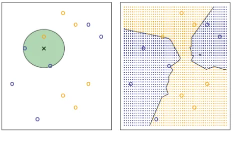
FIGURE2.4: The KNN approach, forK=3 (G. et al.,2013).

Figure 2.5 provides an illustrative explanation of the KNN approach. A set of training data consisting of blue and orange class observations is presented on the left side of the plot. The purpose of this problem is to predict the class (blue or orange) of the black cross labeled data point, given thatKis equal to three. KNN first finds the three observations that are closest to the cross. These neighborhood of three nearest observations is marked by the circle. It consists of two blue points and one orange point, with resulting estimated probability of 2/3 for the blue class and 1/3 for the orange class. Therefore, KNN will predict that the black cross belongs to the blue class. The right-hand side of Figure 2.5 illustrates the result after application of KNN approach at all of the possible values forX1 andX2 with drawn KNN decision boundary. The choice ofKstrongly influences the resulting KNN classifier. We can obtain the optimal model by varying theK value and comparing the training and validation errors. Although this is an overall very simple approach, KNN can often produce surprisingly good results. The summary of some strong and weak points (Lantz,2013) of the KNN algorithm are presented below .

(31)

2.3. Supervised Learning 15 Strengths:

• Simple and effective

• Makes no assumptions about the data distribution • Fast training phase

Weaknesses:

• Slow classification phase

• Does not produce a model as such, which limits the ability to find relationships among features

• Requires a large amount of memory 2.3.3 Random Forests

Bagging or bootstrap aggregation is a method to reduce the variance of the esti-mated prediction function. Bagging seems to be particularly well suited for for high-variance and low-bias procedures, such as trees. In the case of regression problems, we should repeatedly fit the same regression tree to bootstrap sampled versions of the training data, and average the results. For classification, each time a committee of trees votes for the predicted class.

Random Forests (RF) is a machine learning algorithm that take account of all the features at the same time. It focuses only on ensembles of decision trees. RF is a modification of bagging that builds a large collection of de-correlated trees, and then averages them. This method was developed by Leo Breiman and Adele Cutler. The algorithm buildsntreetrees repeating the following steps (Usuelli,2014):

• step1: Subset the data to build the tree by choosing a random row from the datasampsize times. Each row can be chosen more than once and in the end we have a table withsampsizerandom rows.

• step2: Randomly select amtrynumber of features • step3: Build a decision tree based on the sampled data

RF combine versatility and power in a single machine learning approach. Given that an ensemble uses only a small random portion of the full set of features, it can process very big data sets, where such dimensionality might lead to other models failing. Nevertheless, error rates for most learning tasks are almost as good as for any other method. The strengths and weaknesses (Lantz, 2013) of the model are summarized below.

Strengths:

• Selects only the most important features

• Can be used on data with an extremely large number of features or observa-tions

• Performs well on most problems Weaknesses:

• It may require some effort to tune the model to the data • The model is not easily interpretable

(32)

2.3.4 Supervised Self-Organizing Map

Self-Organizing Maps (SOM) are an effective tool for visualization of high-dimensional data. The SOM (also known as Kohonen maps) algorithm was invented by Pro-fessor Teuvo Kohonen back in 1982, aiming to define a neuro-computational bio-plausible model. The SOM produces a nonlinear, ordered, smooth mapping of a high-dimensional data on a regular, low-dimensional (usually 2D) grid (Kohonen, 2001).

The SOM consists of an input level that distributes input data to each node (neu-ron) at the second level, the so-called competitive level. Each of the nodes in the second layer acts as an output node. Each node in the competitive layer is con-nected to other nodes in its neighbourhood. Neurons in the competitive layer have strong connections with the nearest neighbors and weak connections with more dis-tant neurons. Each nodeiin the map has a weight vectorwiand the number of

ele-ments in the weight vector is equal to the number of features in input vector. Each node (neuron)i is defined by a position in a pre-defined grid of fixed dimension. The SOM is continuously updated during the training phase by randomly choosing one input examplexk and applying the following algorithm (Buessler, Urban, and

Gresser,2002; Almendra and Enachescu,2014):

• Choose the winning uniti∗that minimizes the distance||x_k−w_i||

• The weights of units are updated according to following formula:

wi =wi+ρΦ(i,i∗)(x_k−wi), (2.6)

whereρ is the learning rate,Φ()is the neighboring function, which is a monoton-ically decreasing function of the distance between unitsiandi∗. According to this algorithm, the weight vectors of the winner node and its neighbors are updated and, thus, they become more similar to the input vector, while this similarity will decrease for more distant neurons. The weight correction process is repeated itera-tively until all vectors in the training set are presented a sufficient number of times to the network. Nowadays, SOM is most commonly used in the areas of data min-ing, in particular, data visualization, clustering in biomedical analysis, engineering sciences, macroeconomics and finance.

FIGURE2.5: Architecture of the Self-Organizing Map.

The SOM is an unsupervised technique, but there are several supervised vari-ants of SOM such as counter propagation artificial neural network (CP-ANN), su-pervised Kohonen networks (SKN) and XY-Fused networks (XYF). The Susu-pervised Self-Organizing Map (SSOM) can be used for classification problem, where Y =

(33)

2.3. Supervised Learning 17

(Y1,Y2, ...,YC)is a target output withCclasses,X = (X1,X2, ...,XN)is an input

vec-tor with N number of features. Y represents a binary vector containing class in-formation, where only the class index to which it belongs is set to 1. The difference between SOM and SSOM is that an additional vector of class information is included in the training and it introduces an additional factor that organizes the map. This data model allows class information to influence the topological ordering of the map during training process. Then, the trained map is used for predicting the unknown

Ydimension. The extent to which class information affects map can be controlled by class weight, which can be adjusted depending on how class information is used to train the map: a low value causes the map to be close to unsupervised, and a high value may overfit the data (Xiao et al.,2006; Wongravee et al.,2010).

The architecture of the SSOM model for classification problems is a three-layer neural network, as shown in Figure 2.6. The first layer is the input layer which con-sists ofNnodes (neurons) corresponding to the number of features in the input data. The second layer nodes are constructed during training phase and each node repre-sents a reference pattern. The third layer is the output where each node reprerepre-sents a specific class. Each node in the second layer is connected with the first layer nodes through connectionswji. The weight vector wj of the dimension Nrepresents the

reference pattern of thej-th node in the cluster layer. When the model obtains the input and associated target output, the input vectorXi is transmitted to the cluster

layer, and each node in the cluster layer then calculates the degree to which the input vectorXi belongs to clusterj. Next, the system makes a cluster choice by selecting

the winning nodejwith maximum choice function value from all the nodesjin the cluster layer. If the winning nodejbelongs to the correct class defined by the target output vector, the weight vector of the winning node and those of its neighboring nodes whose classes are the same as the winning nodejwill be updated. However, if the winning node does not represent the class to which it belongs, the system will search for the next best cluster nodej∗whose class is the same as the target output (Thammano and Kiatwuthiamorn,2007).

The explanation of the SSOM architecture above explains general model, but there might be some differences in different types of SSOM. In CP-ANN, the winning node on the input layer determines the position of the winning node on the output layer, so, the output layer of the simplified CPN model is developed exclusively by the topology present in the input space. Therefore, the CPN model cannot be consid-ered as a truly supervised method. During the training of the SKN model, the input and output layers must be glued and training process works like in a standard SOM, but the information in the output layer is used to indicate the winning node in the learning phase. The main disadvantage of the SKN network is that the user must de-termine the right balance between input and output objects. Correct scaling of input and output vectors has a huge importance on model creation. Imbalance in inputs and outputs can negatively affect the model efficiency. InXY-Fused networks, the fused similarity is calculated from both input and output layer and is used to deter-mine the position of the winner node. The set of similarities obtained for an object

X and the input map units is combined with the similarities corresponding to the output objectYand the output map such that common winning unit for both maps is determined (Vasighi and Kompany-Zareh,2013; Melssen, Wehrens, and Buydens, 2006).

(34)

FIGURE 2.6: Architecture of the Supervised SOM for classification problem (Thammano and Kiatwuthiamorn,2007).

2.3.5 Cross Validation

The data analysis might face a bias caused by the particular sample chosen. Each class in the data set should be represented in equal proportions in the training and testing sets. If all examples with a certain class were omitted in the training set, the classifier extracted from this data will not work well with examples from this class. A simple way to prevent it, is to use statistical technique called cross-validation. In cross-validation, a fixed number of folds (k) of the data should be chosen. Then, the training sample is divided intoksubsets, each of which has the same number of samples. The classifier is trainedktimes, in each iteration the one of subset is used for testing and the remaining data is used for training. For example, in thei-th iter-ation (i = 1, ...,k) iteration the classifier is trained on all subsets except thei-th one, then, the classification error is computed for thei-th subset. The procedure should be repeatedktimes so that in the end, every instance has been used exactly once for testing. This is calledk-fold cross-validation. Differentk-fold cross-validation exper-iments with the same learning scheme and data might provide different results due to the effect of random variation in choosing the folds (Witten, Eibe, and Hall,2011).

2.4 Review of related works

Financial distress prediction is a well-studied topic. There is no standardized proce-dure to access companies’ full internal data, so, most models proposed in the litera-ture rely on only main financial ratios which are easy to obtain as public companies are bound to disclose their main financial results. There are some rare cases though in which not only financial indicators are used. For instance, Ptak-Chmielewska and Matuszyk (2018) in their work “The importance of financial and non-financial ra-tios in SMEs bankruptcy prediction” (Ptak-Chmielewska and Matuszyk,2018) used financial and non-financial data in their analyses. The usage of non-financial data

(35)

2.4. Review of related works 19 together with financial data improved the results of models which were previously based on only financial indicators. In addition, some researches are trying to deter-mine whether the financial results of bankrupt firms differ based on demographic data. Lukason (2012) used Independent Samples Median Test to check whether me-dians of different pre-bankruptcy financial results changes vary through firm types (Lukason,2012). Based on the data of Estonian bankrupt firms for the period 2002-2009, it was proved, that there are a differences in the financial indicators for differ-ent industries, size groups, bankruptcy years, insolvency types and varying levels of control.

According to my review of the literature, some studies use dimensionality reduc-tion or feature extracreduc-tion techniques as pre-processing step. The study conducted,

inter alia, by Adalessossi (2015) used PCA to explore hidden relationships between variables (Adalessossi,2015). Chen (2011) used PCA for dimensionality reduction in the study “Bankruptcy prediction in firms with statistical and intelligent tech-niques and a comparison of evolutionary computation approaches”. It was identi-fied that with nearly 80% fewer financial ratios, the prediction performance is still able to provide highly-accurate forecasts of financial bankruptcy (Chen,2011). Va-clav and Hampel (2016) used filter based feature selection algorithms like Gain ra-tio, Chi-square and Relief in order to obtain attributes with the best information value(Václav Klepáˇc,2016). A SOM model was used by Kiviluoto (1998) in the pa-per “Predicting bankruptcies with the self-organizing map” as an exploratory pre-processing step to visualize the differences between companies that go bankrupt and those that do not (Kiviluoto, 1998). Arora and Saini (2014) applied Indepen-dent Component Analysis (ICA) on the input data set comprising financial ratios to choose the most significant to be considered as input to the further analysis (Arora and Saini,2014).

Plenty of techniques have been used in bankruptcy prediction. We will dis-cuss most popular algorithms in the remaining part of this section. SVM is one of the most frequently used classification techniques in the area of bankruptcy pre-diction. The studies conducted by Chen (2011) and Kalyan and Amulyashr (2015) analyzed bankruptcy prediction with different machine learning techniques like lo-gistic regression, decision trees, RF, Naive Bayes, neural networks and SVM, the results showed that SVM outperformed other techniques (Chen,2011; Kalyan and Amulyashree,2015). The authors of the paper “Prediction of Bankruptcy with SVM Classifiers Among Retail Business Companies in EU”, Vaclav and Klepac (2016), ap-plied the SVM method with linear, polynomial and radial kernels to obtain the best bankruptcy prediction results (Václav Klepáˇc, 2016). The data used in the study consists of financial data of 850 medium-sized retail business companies in EU from which 48 companies were bankrupt in 2014. One of the questions raised in this pa-per is whether it is possible to predict bankruptcy 1–5 years before the bankruptcy time. The results indicated that the longest prior-to-bankruptcy period models are not efficient enough to predict the bankruptcy. The SVM classifier based on RBF kernel performed best according to accuracy for 1 year-ahead prediction.

Hauser and Booth (2011) investigated the accuracy of bankruptcy prediction us-ing financial ratio data of U.S. firms from 2006 till 2007 (Hauser and Booth,2011). They compared the results of robust logistic regression with the Bianco and Yohai (BY) estimator versus maximum likelihood (ML) logistic regression and BY. With both the 2006 and 2007 data, BY robust logistic regression improved the classifica-tion results of ML logistic regression in the training and testing sets. The study “A Cash Flow Based Model of Corporate Bankruptcy in Australia”, by Jones (2016), em-ploys binary logistic regression to predict corporate bankruptcies in Australia using

(36)

cash flow based ratios (Jones,2016). The results outperformed a logit model esti-mated on Altman Z-score variables.

The Z-score formula was devised in 1968 by Edward I. Altman. This formula is used to predict the probability that a firm will face financial distress. The advantages of this method are that it is easy to calculate and provides quite satisfactory results. Craciun and co-workers (2013) tested the suitability of Altman’s model to predict the financial health of Romanian companies in the period of financial crisis (Cr˘aciun et al., 2013). The data used in the study included financial ratios of 60 Romanian companies for the period between 2005 and 2009. Altman’s model obtained a satis-fying result for the economic period in which this model was developed (1946-1965), however, it failed predicting the bankruptcy of Romanian firms under an unstable economic environment. Adalessossi (2015) applied Altman’s Z-scores to predict the probability of bankruptcy of West African’s firms using the financial statements for 2013. The analysis overall provided fair results (Adalessossi,2015).

Artificial neural networks have performed well in business-related classifica-tion problems including bankruptcy predicclassifica-tion. Arora and Saini (2014) used Fuzzy SVMs to predict financial distress in companies in “Bankruptcy Prediction of Fi-nancially Distressed Companies using Independent Component Analysis and Fuzzy Support Vector Machines”. Surprisingly, Fuzzy SVMs yielded an accuracy of around 94%. Lately, The SOM method has became more popular in classification prob-lems like bankruptcy prediction. Back, Oosterom and Sere (1994) examined the pre-diction power of the SOM algorithm, the backpropagation network and the Boltz-mann Machine. The resultas showed that the backpropagation net performs best in bankruptcy prediction (Back, Oosterom, and Sere, 1994). Serrano-Cinca (1996) describes the usage of SOM for financial health analysis in his work named “Self organizing neural networks for financial diagnosis”. This model was used sepa-rately as well as in combination with other models like Linear Discriminant Anal-ysis and a Multilayer Perceptron artificial neural network. According to Serrano-Cinca, the flexibility of the neural model for combining and adapting to other struc-tures, whether neural or otherwise, guaranteed a bright future for this type of model (Serrano-Cinca, 1996). Kiviluoto (1998) utilized the SOM algorithm in qualitative analysis to visually examine difference between bankrupt and non-bankrupt firms and in the classification analysis as a vector quantizer, to predict financial distress in firms (Kiviluoto,1998).

In this thesis, several machine learning and related algorithms, namely KNN, RF, SVM and supervised SOM will be used to predict the financial distress of U.S. banks for the period 1993-2017. The prediction will be made based on the results of dimen-sionality reduction and feature extraction techniques like PCA and EFA, which will be obtained from the features corresponding to the changes in the financial results of U.S. banks based on three different time periods: a quarter, half-year and a year before bankruptcy.

(37)

21

Chapter 3

Materials and Methods

In this chapter, the data sources are summarily described, followed by the data pre-processing methods and the strategies to increase the interpretability of the data.

3.1 Data Source

The data used in this study was retrieved from the Federal Deposit Insurance Cor-poration (FDIC) database. The FDIC provides the list of U.S. insured banks which went bankrupt during the period 1992-2017. Also, financial organizations insured in FDIC submit quarterly reports with financial results, which are publicly available on the FDIC website. According to FDIC, the total number of the U.S. banks which went bankrupt between 1992-2017 reached 845.

FIGURE3.1: Number of banks which faced financial distress during the 1992-2017 period in the U.S.

All quarterly reports with financial data of banks for the 1992-2016 period were extracted from the FDIC website to be used in the prediction of the financial distress of observed banks during 1994-2017 period. The data for each quarter consists of up to 60 financial reports in CSV format. The number of banks listed in the reports varies from 5,679 up to 13,973.

After merging all financial results for each quarter, we obtained overall 1,034 financial indicators common to all observed time periods. These indicators were used to form exploratory variables by calculating the percentage changes of each

(38)

FIGURE3.2: Total number of banks in U.S. during 1992-2017

financial indicator during one of the three proposed time intervals; therefore, three different data sets with 1,034 features were created.

The final data sample consists of changes in financial results of all bankrupt banks and randomly selected non-bankrupt banks. The formula for computation of changes in financial results is presented below:

Frij =

F_i(j−1)−Fi(j−2)

F_i(j−2)

, (3.1)

where,Frij - changes in financial results of bankifor the periodj;Fi(j−1)- financial results of bankifor the period prior tojperiod;F_i(j−2)– financial results of bankifor the period prior toj−1 period. The periods of calculation might be the following: 1) quarter-based for scenario 1, 2) half-year-based for scenario 2, 1) year-based for scenario 3.

3.2 Data Pre-processing

The data samples for our analyses were built from all bankrupt and randomly lected non-bankrupt banks’ financial results. Non-bankrupt banks’ data was se-lected from the same period that for bankrupt banks, and the proportion of bankrupt-to-non-bankrupt is equal to 1/5. Given the requirement that the financial history of the enterprise be known well enough, if there was no data available for an observed period before the bankruptcy date of the company, the bank was excluded from the analyzed sample. As mentioned, the data sets for all three scenarios consist of 1,034 exploratory variables, including the demographic data.

In the data pre-processing step, the main concern was to check if the data set had any missing values. The final data sets were checked for missing values and all variables with more than 90% of missing values were removed from them. The remaining missing values, even if this is not the optimal procedure, were replaced with “0” values. After removal, the total number of variables decreased to only

(39)

3.2. Data Pre-processing 23

TABLE3.1: Groups of exploratory variables.

Group name Number of variables

Assets and Liabilities 30

Performance and Condition Ratios 27

Total Deposits 13

Income and Expense 12

Net Loans and Leases 9

Securities 3

Changes in Bank Equity Capital 2

Total Interest Income 2

1-4 Family Residential Net Loans and Leases 1 Additional Noninterest Expense 1

Cash and Balances Due 1

Maturity & Repricing for Loans and Leases 1

Nontransaction Accounts 1

Time Deposits at the $100,000 Threshold 1

Total Interest Expense 1

Transaction Accounts 1

Total 106

139 in all scenarios. As demographic data is not used in further analysis, the cor-responding columns were also removed. In the end, the data set was composed of 106 exploratory variables and 1 response variable. The response variable is cat-egorical, where the value “1” refers to bankrupt entities, and “0” corresponds to non-bankrupt entities.

In order to simplify the visualization of the data, exploratory variables were split into 16 groups based on the definition provided by FDIC reports. The groups of data are presented in full in Table 3.1. The full list of explanatory variables for each scenario with the corresponding groups are presented in AppendixA, AppendixB

and AppendixC. As some of groups of data were subgroups of other groups, the variables were merged into 6 “super-groups” only for visualization purposes.

The data sets were checked for multi-collinearity, and the “Variance Inflation Factors” (VIF) test detected very strong multi-collinearity in all three scenarios. 3.2.1 Scenario 1: Quarterly changes in financial results

This data set was built by computing the percentage of change in financial results between 1 and 2 quarters prior to the possible bankruptcy date.

The data from FDIC reports from 4Q 1992 till 3Q 2017 were used to forecast bankruptcy for the period from 2Q 1993 till 4Q 2017.

The data set consists from 399 observations of bankrupt banks and 1,995 obser-vations of non-bankrupt banks. The original total number of variables including demographic data is equal to 1,034. After the removal of variables with too many missing values, the total number of variables decreased to 139. The final data set af-ter demographic data removal consisted of 106 exploratory variables and 1 response variable. The data set can be considered as medium-sized, consisting of just 2,394 entries.

The boxplots of variables from the “Loans and Leases” group, broken down by class value, are presented in Figure 3.3. The boxplots of the remaining groups are

(40)

FIGURE3.3:Loans and Leasesgroup boxplots: Scenario 1

FIGURE3.4:Loans and Leasesgroup density plots: Scenario 1

presented in AppendixDto avoid cluttering the document. There is a common pat-tern for some of the variables: the bankrupt banks’ exploratory mean values of the variables are smaller than zero, which means negative percentage change in finan-cial results, while the mean values of exploratory variables of non-bankrupt entities are close to 0 or slightly over 0.

The density plots of the variables were broken down by class value. It helped to understand the overlap of classes for any given attribute. Figure 3.4 shows the density plots of the “Loans and Leases” group variables. The red colored part of the density plot presents bankrupt entities. As we can see, the density of bankrupt and non-bankrupt entities are almost equal. Also, we should take into account that the number of bankrupt banks is 5 times lower than the non-bankrupt banks in the data set. In the density plots, we can see that those of bankrupt banks are shifted to the left, as related to the non-bankrupt banks. The density plots of the remaining groups of variables are presented in AppendixEfor further detail.

(41)

3.2. Data Pre-processing 25

FIGURE3.5:Total Depositsgroup boxplots: Scenario 2

3.2.2 Scenario 2: Half-year changes in financial results

The data set for this scenario was built from the percentage changes in financial results between half-year and 1 year prior to the possible bankruptcy date. The data from FDIC reports from 4Q 1992 till 2Q 2017 were used to forecast bankruptcy for the period from 4Q 1993 till 4Q 2017.

FIGURE3.6:Total Depositsgroup density plots: Scenario 2

If there was no data available for 1 year before the bankruptcy date of the com-pany, the bank was excluded from the sample. The data set consisted of 390 ob-servations of bankrupt and 1,950 non-bankrupt banks’ results, with an overall 2,340 entries.

The boxplots of variables from the “Total Deposits” group, broken down by class value are presented in Figure 3.5, remaining boxplots are presented in AppendixF. The density plot was also broken down by class value. Figure 3.6 shows the density plots of the “Total Deposits” group variables. The red colored part of the plot repre-sents bankrupt banks. The density of bankrupt and non-bankrupt entities are almost

(42)

equal except that the density plots of bankrupt banks are shifted to the left related to the non-bankrupt banks. The density plots of remaining groups of variables are presented in AppendixG.

FIGURE 3.7: Performance and Condition Ratios group boxplots: Sce-nario 3

3.2.3 Scenario 3: Yearly changes in financial results

The data set for this scenario represents the percentage changes in financial results between 1 year and 2 years before possible bankruptcy date. The data from FDIC reports from 4Q 1992 till 4Q 2016 were used to forecast bankruptcy for the period from 4Q 1994 till 4Q 2017. The data set includes 375 entries of bankrupt banks and 1,875 of non-bankrupt banks, which is 2,250 entries in total.

FIGURE3.8:Performance and Condition Ratiosgroup density plots: Sce-nario 3

The boxplots and density plots of variables from the “Performance and Con-dition Ratios” group, broken down by class value are presented in Figure 3.7 and

(43)

3.3. Dimensionality reduction and feature extraction 27 Figure 3.8 respectively. Remaing boxplots and density plots are presented in the AppendixHand AppendixI.

3.3 Dimensionality reduction and feature extraction

The paragraphs below describe the steps and calculations performed to apply the two dimensionality reduction and feature extraction methods described in the pre-vious chapter: PCA and EFA.

3.3.1 Principal Components Analysis

PCA was conducted on normalized data. The correct number of components in PCA was identified based on the variance threshold. The number of first components which overall explain about 90% of variance in data was retained for further analy-sis. PCA results are determined by the dimension of the data set under study. In this case, the data sets consist of 107 exploratory variables, so, 107 PCs were originally computed.

Scenario 1: Quarterly changes in financial results

In this study, as mentioned, the threshold used was set to 90%. Even by keeping the 42 PCs, totalling a 90.12% of variability in the data, we achieved a good dimension-ality reduction by explaining the variability of the 107 variables with just 42 in the new space.

FIGURE3.9: Scree plot: Scenario 1

The scree plot of the eigenvalues found after performing PCA on our data set is presented in the Figure 3.9. The total number of dimensions retained doesn’t satisfy the Kaiser criterion. However, the lowest eigenvalue is equal to 0.76, which is still quite sufficient.

The first 3 PCs explain about 34.25% of the total variance. Therefore, I plotted each individual in these three dimensions as shown in Figure 3.10. The individuals are grouped by class, the blue triangles represent the non-bankrupt entities, while yellow circles represent the bankrupt banks. It seems that some bankrupt banks have high correlation with the third dimension while the non-bankrupt banks don’t have

(44)

or have very low correlation with the third dimension. However, non-bankrupt banks seem to have mostly positive correlation with the first PC, while, bankrupt banks have negative correlation with the first PC. Also, We see that there is no clear-cut linear separation between the bankrupt and non-bankrupt banks in the first three dimensions.

FIGURE3.10: The first 3 dimensions obtained from PCA: Scenario 1.

3.3.2 Scenario 2: Half-year changes in financial results

The scree plot of the PCA of the data set composed from the half-year changes in financial results is presented in the Figure 3.11. The red circle on the plot denotes the number of components retained for further analysis.

Predicting financial distress through machine learning

M

T

Predicting Financial Distress Through

Machine Learning

Declaration of Authorship

Abstract

Acknowledgements

Contents

List of Figures

List of Tables

List of Abbreviations

Chapter 1

Introduction

1.1

Motivation

1.2

Goals and Research Questions

1.3

Outline

Chapter 2

Background

2.1

Banking

2.2

Dimensionality reduction and feature extraction

2.3

Supervised Learning

∑

2.4

Review of related works

Chapter 3

Materials and Methods

3.1

Data Source

3.2

Data Pre-processing

3.3

Dimensionality reduction and feature extraction