DOI 10.1007/s11590-017-1107-z
S H O RT C O M M U N I C AT I O N
On the comparison of initialisation strategies in
differential evolution for large scale optimisation
Eduardo Segredo1 · Ben Paechter1 · Carlos Segura2 · Carlos I. González-Vila3
Received: 24 March 2016 / Accepted: 6 January 2017
© The Author(s) 2017. This article is published with open access at Springerlink.com
Abstract Differential Evolution(de) has shown to be a promising global
optimi-sation solver for continuous problems, even for those with a large dimensionality. Different previous works have studied the effects that a population initialisation strat-egy has on the performance of dewhen solving large scale continuous problems,
and several contradictions have appeared with respect to the benefits that a particu-lar initialisation scheme might provide. Some works have claimed that by applying a particular approach to a given problem, the performance ofdeis going to be
bet-ter than using others. In other cases however, researchers have stated that the overall performance ofdeis not going to be affected by the use of a particular initialisation
method. In this work, we study a wide range of well-known initialisation techniques for
de. Taking into account the best and worst results, statistically significant differences
among considered initialisation strategies appeared. Thus, with the aim of increasing the probability of appearance of high-quality results and/or reducing the probability
B
Eduardo Segredo [email protected] Ben Paechter [email protected] Carlos Segura [email protected] Carlos I. González-Vila [email protected]1 School of Computing, Edinburgh Napier University, Edinburgh, Scotland, UK 2 Área de Computación, Centro de Investigación en Matemáticas, Callejón Jalisco s/n,
Mineral de Valenciana, Guanajuato 36240, Mexico
of appearance of low-quality ones, a suitable initialisation strategy, which depends on the large scale problem being solved, should be selected.
Keywords Differential evolution·Initialisation strategies·Large scale continuous optimisation
1 Introduction
Differential Evolution(de) is one of the most widely used meta-heuristics to deal with
continuous optimisation problems [17]. Due to its simplicity and efficiency, it has not only been applied to benchmark problems, but also to a wide range of real-world appli-cations regarding electrical and power systems, robotics, and bio-informatics, among others [2]. Moreover,deand its variants have usually been one of the best
perform-ing approaches in different contests, such as the competition onLarge Scale Global Optimisation(lsgo) organised in different editions of theCongress on Evolutionary Computation(cec) [10].
Regardinglarge scaleproblems, i.e., problems with a large dimensionality, typi-cally more than 100 decision variables [6], a significant number of works have tried to modify different aspects of de for searching the vast decision space in a more
efficient way [2]. For instance, in [12], a novel proposal that groups dependent deci-sion variables in different sets was combined withde, being the latter responsible for
optimising each set of variables separately. Another work proposed a linearly scalable exponential crossover operator that provided promising results considering a recent set of scalable benchmarks [19]. Recently, two novel schemes that improve the trial vector generation strategy ofdewere proposed, which showed to increase the performance
of that algorithm when dealing with large scale problems [13]. Finally, the analysis of different strategies for initialising the population ofdewith the aim of improving its
performance with large scale optimisation problems has gained a noticeable popularity in recent years [5,18].
Some controversies have arisen concerning the benefits that a particular initial-isation strategy, applied together with de, might provide when solving large scale
problems [5]. The common belief is that some initialisation strategies can improve the performance ofdefor solving problems with a high dimensionality. For instance, the
main conclusion given in [6] is that, in opposition to the application of basic random number generators as initialisation strategies, other more advanced methods should be considered in order to increase the performance ofdewhen dealing with large scale
problems, with the most suitable initialiser depending on the problem at hand. In a more recent work [5] however, authors claimed that the initialisation approach does not significantly affect the performance ofde. In that paper, the behaviour of several
advanced initialisation methods with different features was analysed when dealing with a set of large scale problems. Those initialisation strategies were combined with the best performing configuration found for one of the most widely useddevariants.
Although a few differences among initialisation techniques appeared in some cases when functions were analysed separately, all initialisation approaches performed in a statistically similar fashion taking into account the test suite as a whole.
In the current work, we try to shed some light on the above, by performing a novel study which consists of analysing the behaviour of a wide range of initialisation strate-gies in the overall, best, and worst cases. Those initialisation mechanisms are applied with the aforementioned best parameterisation ofdeto the same set of large scale
problems considered in [5]. We show that initialisation strategies present a consider-ably larger number of statistically significant differences for the best and worst cases in comparison to the overall case, and therefore, a proper mechanism should be selected with the aim of increasing the probability of appearance of high-quality results and/or reducing the probability of appearance of low-quality ones, especially in cases where a high number of executions is not feasible.
The rest of this paper is organised as follows.deand the particular variant applied
herein are described in Sect.2. Section3is focused on introducing the initialisation strategies considered for our study. Afterwards, in Sect.4, the different experiments conducted are exposed, together with their discussion. Finally, some conclusions and lines of future work are shared in Sect.5.
2 Differential evolution
deis a stochastic direct search method especially suited for continuous global
opti-misation [17]. Inde, the decision variables of a given problem are defined by a vector X= [x1,x2, . . . ,xi, . . . ,xD], beingDthe number of decision variables or the
dimen-sionality of the problem, and everyxi=1...Da real number. As we previously mentioned,
the term large scale problems is used to refer to those optimisation problems with a large dimensionality, typically D > 100. The quality of each vectorXis given by the objective function f(X)(f : Ω ⊆ RD → R). The goal of the global optimi-sation, considering a minimisation problem, is thus to find a vectorX∗ ∈Ω where
f(X∗)≤ f(X)holds for allX∈Ω. In the particular case of box-constrained contin-uous optimisation problems, the feasible regionΩ is defined by particular values for the lower (ai) and upper (bi) bounds of each variable, i.e.,Ω =iD=1[ai,bi].
Taking into account the most widely used nomenclature forde[17], i.e.,de/x/y/z,
wherexis the vector to be mutated,ydefines the number of difference vectors used, and
zindicates the crossover scheme, in this work we applied the approachde/rand/1/bin.
We selected this variant due to its simplicity and popularity. The operation of this
devariant is as follows. First of all, a population P = [X1,X2, . . . ,Xj, . . . ,XN P]
withN P individuals, also called vectors in the field ofde, is initialised by using a
particular strategy. Each individual comprisesDdecision variables. The value of the decision variableibelonging to the individualXjis denoted byxj,i. Then, successive
iterations are evolved by executing the following steps. For each vector Xj in the
current population, calledtarget vector, a newmutant vector Vj is created using a
mutant vector generation strategy. Several mutant vector generation strategies have been devised [2]. In our case, we applied the rand/1 scheme, which is probably the most popular one. The mutant vectorVj for target vectorXjis thus created as shown
in Eq.1, wherer1,r2, andr3are mutually exclusive integers chosen at random from the range[1,N P]. Furthermore, they are all different from the indexj. Themutation scale factor Fallows the exploration and exploitation abilities ofdeto be balanced.
Vj =Xr3+F×(Xr1−Xr2) (1)
After applying the mutant vector generation strategy, the mutant vector is combined with the target vector to generate thetrial vectorUjthrough a crossover operator. The
combination of the mutant vector generation strategy and the crossover operator is usually referred to as thetrial vector generation strategy. The most commonly applied operator for combining the target and mutant vectors—and the one considered in this paper—is thebinomial crossover(bin). The crossover operation is controlled by means of the crossover rateC R. The binomial crossover generates a trial vector as shown in Eq.2. A uniformly distributed random number in the range[0,1]is given byr andj,i,
andir and∈ [1,2, . . . ,D]is an index selected in a random way that ensures that at least
one variable is propagated from the mutant vector to the trial one. For the remaining cases, the probability of the variable being inherited from the mutant vector isC R. Otherwise, the variable of the target vector is taken into consideration.
uj,i =
vj,i i f (r andj,i ≤ C R or i = ir and)
xj,i ot herwi se (2)
The trial vector generation strategy, as described above, might generate vectors outside the feasible region Ω. One of the most widely used schemes is based on randomly reinitialising the infeasible values in their corresponding feasible ranges, and it is the one applied herein. Finally, after generatingN Ptrial vectors, each one is compared against its corresponding target vector. For each pair, the one that minimises the objective function is selected to survive. In case of a tie, in our implementation the trial vector survives.
3 Initialisation strategies for differential evolution
A wide range of initialisation strategies have been proposed in order to improve the results obtained byde[2,5,18]. In the current work, we compared the same set of
initialisation strategies considered in [5], which are introduced herein.
Pseudo-Random Number Generators (prngs) and Chaotic Number Generators
(cngs) are one of the most frequently used approaches for initialising a population
of individuals [11,15]. In the case ofprngs, one of the most popular methods is Mersenne Twister(mt) [9], which is included as a typicalprngon a large number
of programming languages. Particularly, we used the variant that provides a period of 219937and 623-dimensional equidistribution with 32-bit accuracy. Regardingcngs, we
consideredTent Map(tm) [3]. This approach produces a chaotic sequence of numbers
uniformly distributed in the range[0,1], and has shown some benefits, like a higher iterative speed, with respect to othercngs, such asLogistic Map[3].
The aforementioned types of schemes take into account both randomness and uni-formity to generate the initial population. There exist other kinds of schemes however, that only consider uniformity, and therefore, are usually deterministic. From among those strategies, we applied the methodsSobol Set(ss) [1] andGood Lattice Points
(glp) [16], which are able to provide a set of points well distributed in the decision
space.
Finally, Opposition-based Learning(obl) mechanisms as initialisation methods
fordehave gained a significant popularity in recent years [18]. Instead of considering
randomness and/or uniformity,oblgenerates an initial population and calculates the
opposite one with the aim of selecting the fittest individuals from both populations as the starting set. There are different variants ofoblschemes [18]. In addition to the
approaches considered in [5], i.e.,oblandQuasi-Opposition-based Learning(qobl),
we also appliedQuasi-Reflection Opposition-based Learning(qrobl) herein, since a
recent work [4] stated that the quasi-reflected opposition individual is more likely to be closer to the optimal solution than the opposition and quasi-opposition individuals.
4 Experimental evaluation
This section is devoted to describe the experiments conducted with the version ofde
introduced in Sect.2integrated with the different initialisation strategies depicted in Sect.3.
Experimental method
The approachde/rand/1/bin, as well as the initialisation strategies considered, were
implemented by using theMeta-heuristic-based Extensible Tool for Cooperative Opti-misation(metco) [7]. Tests were run onTeideHigh Performance Computing facilities,
which are composed of 1100 Fujitsu® computer servers, with a total of 17800 com-puting cores and 36tbof memory. Since all experiments used stochastic algorithms,
each execution was repeatednum Rep =3×10³times, with the aim of comparing the different initialisation strategies with enough statistical confidence. With respect to the former, comparisons were carried out by applying the following statistical anal-ysis [14]. First, aShapiro-Wilk testwas performed to check whether the values of the results followed a normal (Gaussian) distribution or not. If so, theLevene testchecked for the homogeneity of the variances. If the samples had equal variance, ananova test was done. Otherwise, aWelch test was performed. For non-Gaussian distribu-tions, the non-parametric Kruskal-Wallistest was used. For all tests, a significance levelα=0.05 was considered.
Problem set
Experiments were carried out using a set of scalable continuous optimisation problems proposed incec’13 for itslsgocompetition [8]. It is important to remark that this set
of functions is the latest benchmark suite provided for large scale global optimisation in the field of thecec. Consequently, it was also considered for thelsgo
competi-tion organised duringcec’15.1 The set is composed of 15 functions (f1–f15) with
different features: fully-separable functions (category 1: f1–f3), partially additively separable functions (category 2: f4–f11), overlapping functions (category 3: f12–f14), and a non-separable function (category 4: f15). Following the indications given for 1 We should note that, although special sessions onlsgowere proposed forcec’14 andcec’16, the
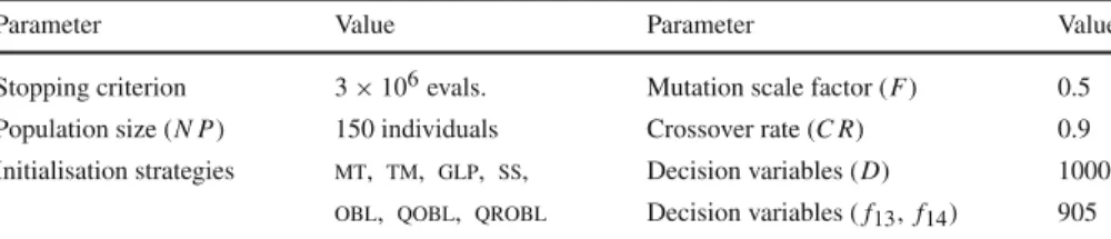
Table 1 Different parameterisations of the schemede/rand/1/bin
Parameter Value Parameter Value
Stopping criterion 3×10⁶evals. Mutation scale factor (F) 0.5 Population size (N P) 150 individuals Crossover rate (C R) 0.9 Initialisation strategies mt, tm, glp, ss, Decision variables (D) 1000
obl, qobl, qrobl Decision variables (f13,f14) 905
the different editions of thelsgo competition, in the current work, the number of
decision variablesDwas fixed to 1000 for all the aforementioned functions, with the exception of problems f13and f14, whereDwas fixed to 905 decision variables due to overlapping subcomponents.
Parameters
The experiments conducted applied a common parameterisation for different config-urations of the schemede/rand/1/bin, which can be observed in Table1. The only
difference among configurations resides on the initialisation strategy used. In pre-vious work [5], a configuration of the scheme de/rand/1/bin using those parameter
values, from among a candidate pool with more than 80 different configurations of that approach, was able to provide the best overall results for problems f1–f15 with 1000 decision variables. That is the reason why we have selected those values for the parametersN P,F, andC R. Finally, rules of thelsgocompetition indicate that
the stopping criterion has to be fixed to a maximum number of 3×10⁶ function evaluations. In order to perform the analyses,dewas applied with each considered
initialisation strategy to each of the 15 benchmark problems, thus giving a total num-ber of 3.15×10⁵runs. Following the recommendations given in [5,10], Eq.3was applied to assign a seeds(i)to thei-th run of everydeconfiguration, regardless of
the initialisation method.
s(i)=i ∀i ∈ {1,2, . . . ,num Rep} (3) Table2 shows rankings of the considered initialisation strategies when the best 300 and the worst 300 executions, i.e., those with the lowest and highest values of the objective function at the end of the runs, respectively, are taken into account. Results regarding all the executions are also shown. In order to calculate rankings the following steps were performed. First, the number of approaches that a particular strategy statistically outperformed (↑), as well as the number of times that it was statistically outperformed (↓) by the remaining schemes, considering all problems, were calculated by applying the statistical procedure explained at the beginning of the current section. Approach A statistically outperforms scheme B if there exist statistically significant differences between them, i.e., if the p-value is lower than
α = 0.05, and if at the same time, A provides a lower mean and median of the objective value thanB, since we are dealing with minimisation problems. Afterwards, the score assigned to a strategy is given by the difference between the number of schemes it was able to beat and the number of schemes that were able to beat it.
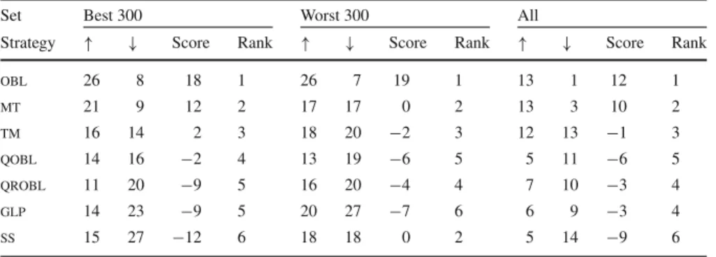
Table 2 Ranking of initialisation strategies considering the best 300 and the worst 300 executions for problems f1–f15
Set Best 300 Worst 300 All
Strategy ↑ ↓ Score Rank ↑ ↓ Score Rank ↑ ↓ Score Rank
obl 26 8 18 1 26 7 19 1 13 1 12 1 mt 21 9 12 2 17 17 0 2 13 3 10 2 tm 16 14 2 3 18 20 −2 3 12 13 −1 3 qobl 14 16 −2 4 13 19 −6 5 5 11 −6 5 qrobl 11 20 −9 5 16 20 −4 4 7 10 −3 4 glp 14 23 −9 5 20 27 −7 6 6 9 −3 4 ss 15 27 −12 6 18 18 0 2 5 14 −9 6
Results are also shown considering all executions
Finally, a ranking is established by sorting strategies in descending order taking into account the scores assigned.
If we consider the whole set of executions, the best performing overall approach was
obl, although followed bymtwith a similar score. In this case, it can be observed that
scores assigned to both aforementioned approaches were lower than those assigned to the first-ranked scheme in the best and worst cases. This means that, if all executions are taken into account, the number of differences among initialisation strategies (122 cases out of 630) significantly decreases in comparison to the number of differences that appears regarding the best (234 cases) and the worst results (256 cases). Furthermore, since two methods obtained similar scores, no initialisation strategy was able to provide a clear advantage with respect to the remaining ones when considering the set of problems as a whole. As a result, it might seem that the initialisation technique does not affect the overall performance ofdewhen solving large scale problems. The above
agrees with the conclusions given in [5].
Nevertheless, it can be observed thatobl was the best performing initialisation
strategy in cases when the best and the worst 300 executions were analysed, since it obtained significantly better scores than the remaining approaches. The methodobl
was statistically better in a larger number of cases than the remaining strategies, while it was statistically worse in a lower number of cases when compared to the remaining schemes. By the application ofoblas an initialisation technique, we therefore might
increase/reduce the probability of appearance of high-quality/low-quality executions when usingdefor solving large scale continuous optimisation problems. A more
in-depth analysis of this method however, should be carried out for each problem, with the aim of providing more evidence of its advantages and drawbacks.
4.1 Analysis of the schemeoblconsidering all the results
This section focuses on comparing the approachoblwith respect to the remaining
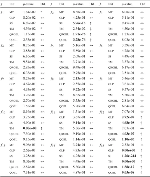
strategies when considering all the executions. Table3shows, for each problem, the
Table 3 Statistical comparison betweenobland the remaining strategies considering problems f1–f15
and all executions
f Init. p-value Dif. f Init. p-value Dif. f Init. p-value Dif.
f1 mt 1.84e-02 * f2 mt 8.58e-01 ↔ f3 mt 6.08e-01 ↔
glp 8.20e-02 ↔ glp 4.25e-01 ↔ glp 5.11e-01 ↔
ss 6.89e-02 ↔ ss 5.96e-15 ↑ ss 9.45e-01 ↔
tm 4.56e-02 * tm 2.34e-02 ↓ tm 4.50e-01 ↔
qrobl 1.13e-01 ↔ qrobl 1.91e-76 ↑ qrobl 1.23e-01 ↔
qobl 2.55e-01 ↔ qobl 3.78e-76 ↑ qobl 8.03e-01 ↔
f4 mt 8.73e-01 ↔ f5 mt 5.16e-01 ↔ f6 mt 3.59e-01 ↔
glp 3.85e-01 ↔ glp 5.89e-01 ↔ glp 4.28e-01 ↔
ss 6.16e-01 ↔ ss 2.09e-01 ↔ ss 4.49e-01 ↔
tm 9.54e-01 ↔ tm 3.71e-01 ↔ tm 3.37e-01 ↔
qrobl 2.83e-01 ↔ qrobl 9.49e-01 ↔ qrobl 6.17e-01 ↔
qobl 6.38e-01 ↔ qobl 9.75e-01 ↔ qobl 3.51e-01 ↔
f7 mt 8.27e-01 ↔ f8 mt 2.13e-01 ↔ f9 mt 5.46e-01 ↔
glp 4.67e-01 ↔ glp 2.55e-01 ↔ glp 3.61e-01 ↔
ss 4.33e-01 ↔ ss 9.22e-01 ↔ ss 9.57e-01 ↔
tm 3.28e-01 ↔ tm 8.62e-01 ↔ tm 5.30e-01 ↔
qrobl 2.70e-01 ↔ qrobl 5.55e-01 ↔ qrobl 2.81e-01 ↔
qobl 1.58e-01 ↔ qobl 5.20e-01 ↔ qobl 6.64e-01 ↔
f10 mt 8.16e-01 ↔ f11 mt 1.51e-01 ↔ f12 mt 7.07e-01 ↔
glp 3.25e-01 ↔ glp 3.67e-01 ↔ glp 2.92e-07 ↑
ss 4.90e-01 ↔ ss 9.14e-01 ↔ ss 4.68e-08 ↑
tm 0.00e+00 ↑ tm 5.36e-01 ↔ tm 7.03e-01 ↔
qrobl 7.30e-01 ↔ qrobl 9.19e-01 ↔ qrobl 4.03e-07 ↑
qobl 9.15e-01 ↔ qobl 1.14e-01 ↔ qobl 1.10e-03 ↑
f13 mt 9.96e-01 ↔ f14 mt 3.74e-01 ↔ f15 mt 2.33e-01 ↔
glp 2.62e-01 ↔ glp 4.73e-01 ↔ glp 0.00e+00 ↑
ss 3.25e-01 ↔ ss 4.25e-01 ↔ ss 1.26e-214 ↑
tm 8.02e-01 ↔ tm 4.48e-01 ↔ tm 0.00e+00 ↑
qrobl 2.87e-01 ↔ qrobl 5.80e-01 ↔ qrobl 1.58e-12 ↑
qobl 7.31e-01 ↔ qobl 4.87e-01 ↔ qobl 9.05e-08 ↑
Data in boldface show those cases where OBL statistically outperformed other initialisation strategy, i.e., where an↑is also shown in columns called “Dif”
remaining approaches. It also shows cases for which obl was able to statistically
outperform other strategy (↑), cases where other strategy outperformedobl(↓), and
cases where statistically significant differences betweenobland the corresponding
method did not arise (↔). Finally, in cases where statistically significant differences betweenobland the corresponding scheme appeared, but one approach obtained the
lowest mean, while the other one provided the lowest median, an ‘*’ is shown. It can be observed that in 10 out of 15 problems, no statistically significant differences
appeared betweenobland the remaining initialisation strategies. This confirms our
previous statement concerning the lack of differences between initialisation methods when the overall results are considered. Generally speaking, there was no strategy that clearly provided better results than the remaining ones regardless of the addressed problem. Despite that, some differences arose in some cases.oblwas better than
sev-eral approaches when solving functions f2, f10, f12, and f15, with each one belonging to a different category. For instance, in the case of the non-separable function f15,obl
showed a clear superiority together withmt. Only in the case of function f2oblwas
statistically worse than another scheme (tm).
4.2 Analysis of the schemeoblconsidering the best results
This section is devoted to compare the initialisation scheme obl in regard to the
remaining approaches when the best 300 executions are considered. Results of this analysis are shown in Table4.
It is important to remark that, taking into account the best 300 executions, differ-ences betweenobland the remaining methods appeared in 11 out of 15 problems,
being this a significant increase concerning the previous analysis of the overall results.
obldid not present statistically significant differences with any other approach for
functions f4, f5, f9, and f11. At the same time, in 8 out of 15 problems,oblwas able
to outperform other strategies, and in 4 out of those 8 functions, it was not worse than any other initialisation strategy. Considering function f14, for example,oblwas
sta-tistically better, together withmtandss, than the remaining schemes. This means that,
if users would like to increase the probability of appearance of high-quality results when solving problem f14, they should initialise the population ofdewith one of
those three strategies. Moreover, depending on the problem being solved, the most suitable initialisation strategy changes. For instance, taking into account function f8, the best performing scheme wasobl, together withmtandglp, while in the case of
f7,qoblprovided the best performance.
4.3 Analysis of the schemeoblconsidering the worst results
In this section, we carry out a similar analysis than the one exposed in the previous section, but in this case, we compare the strategyoblwith respect to the remaining
approaches when considering the worst 300 executions. Results of this study are shown in Table5.
In the worst case, differences betweenobland the remaining methods appeared in
14 out of 15 problems. As in the best case, this is a significant increase of differences in comparison to the study considering all executions. Only in the case of function f8,
obldid not present statistically significant differences with any other approach. In 11
out of 15 problems,oblwas able to outperform other strategies. In fact, in 10 out of
those 11 functions, it was not worse than any other initialisation strategy. For instance, considering function f2,oblwas statistically better, together withmtandtm, than the
remaining schemes. This means that, in the worst case,dewould attain better results
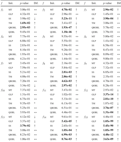
Table 4 Statistical comparison betweenobland the remaining strategies considering problems f1–f15
and the best 300 executions
f Init. p-value Dif. f Init. p-value Dif. f Init. p-value Dif.
f1 mt 3.06e-01 ↔ f2 mt 4.78e-02 ↑ f3 mt 2.96e-02 ↑
glp 4.32e-01 ↔ glp 2.96e-01 ↔ glp 1.45e-01 ↔
ss 3.98e-02 ↓ ss 5.23e-11 ↑ ss 3.90e-04 ↑
tm 1.69e-02 ↑ tm 3.41e-07 ↓ tm 3.06e-01 ↔
qrobl 2.95e-03 ↑ qrobl 1.93e-47 ↑ qrobl 5.78e-02 ↔
qobl 9.45e-01 ↔ qobl 1.18e-46 ↑ qobl 3.79e-01 ↔
f4 mt 7.75e-01 ↔ f5 mt 9.55e-01 ↔ f6 mt 5.80e-02 ↔
glp 6.88e-02 ↔ glp 5.55e-01 ↔ glp 1.41e-02 ↓
ss 2.83e-01 ↔ ss 5.94e-01 ↔ ss 6.58e-01 ↔
tm 8.10e-01 ↔ tm 9.28e-01 ↔ tm 8.47e-01 ↔
qrobl 1.93e-01 ↔ qrobl 1.34e-01 ↔ qrobl 8.09e-02 ↔
qobl 4.21e-01 ↔ qobl 1.44e-01 ↔ qobl 9.00e-01 ↔
f7 mt 3.45e-01 ↔ f8 mt 2.16e-01 ↔ f9 mt 4.32e-01 ↔
glp 7.59e-01 ↔ glp 5.84e-02 ↔ glp 7.32e-01 ↔
ss 5.21e-02 ↔ ss 2.81e-03 ↑ ss 6.85e-01 ↔
tm 4.08e-01 ↔ tm 2.86e-02 ↑ tm 2.35e-01 ↔
qrobl 7.20e-01 ↔ qrobl 4.62e-03 ↑ qrobl 4.70e-01 ↔
qobl 3.34e-02 ↓ qobl 2.97e-02 ↑ qobl 8.28e-01 ↔
f10 mt 7.37e-02 ↔ f11 mt 3.47e-01 ↔ f12 mt 2.97e-02 ↓
glp 1.31e-01 ↔ glp 1.02e-01 ↔ glp 3.37e-14 ↑
ss 6.75e-01 ↔ ss 5.33e-01 ↔ ss 2.81e-10 ↑
tm 9.35e-03 * tm 6.13e-01 ↔ tm 1.87e-02 ↓
qrobl 5.25e-01 ↔ qrobl 6.51e-01 ↔ qrobl 3.76e-07 ↑
qobl 3.93e-01 ↔ qobl 4.46e-01 ↔ qobl 1.31e-04 ↑
f13 mt 4.12e-02 ↓ f14 mt 9.61e-01 ↔ f15 mt 4.46e-01 ↔
glp 3.37e-02 ↓ glp 5.42e-05 ↑ glp 1.05e-99 ↑
ss 3.79e-02 ↑ ss 2.65e-01 ↔ ss 5.45e-90 ↑
tm 3.08e-01 ↔ tm 1.05e-04 ↑ tm 1.05e-99 ↑
qrobl 8.23e-02 ↔ qrobl 6.99e-03 ↑ qrobl 4.48e-12 ↑
qobl 1.06e-01 ↔ qobl 8.76e-03 ↑ qobl 3.63e-09 ↑
Data in boldface show those cases where OBL statistically outperformed other initialisation strategy, i.e., where an↑is also shown in columns called “Dif”
the problem being solved, as in the best case, the most suitable initialisation strategy changes. Taking into account function f9, for example, the best performing scheme wasobl, together withtm,glpandqrobl, while in the case of f14,ssprovided the
best performance.
Finally, it is worth mentioning that, if we consider the best and worst cases simul-taneously, there exist two problems (f3and f15) for whichobl, and other schemes,
were the best performing initialisation approaches. The above means that those ini-tialisation strategies allow the probability of appearance of high-quality results to be
Table 5 Statistical comparison betweenobland the remaining strategies considering problems f1–f15
and the worst 300 executions
f Init. p-value Dif. f Init. p-value Dif. f Init. p-value Dif.
f1 mt 5.99e-03 ↑ f2 mt 3.64e-01 ↔ f3 mt 5.52e-01 ↔
glp 3.17e-01 ↔ glp 3.46e-05 ↑ glp 9.69e-01 ↔
ss 1.07e-02 ↑ ss 7.89e-12 ↑ ss 8.73e-02 ↔
tm 2.78e-01 ↔ tm 2.15e-01 ↔ tm 9.76e-04 ↑
qrobl 5.69e-02 ↔ qrobl 1.14e-46 ↑ qrobl 7.93e-02 ↔
qobl 1.44e-03 ↑ qobl 6.32e-47 ↑ qobl 8.97e-01 ↔
f4 mt 2.26e-01 ↔ f5 mt 3.40e-01 ↔ f6 mt 1.66e-02 ↑
glp 3.07e-02 ↑ glp 1.11e-05 ↑ glp 6.30e-01 ↔
ss 9.43e-01 ↔ ss 6.11e-06 ↑ ss 8.42e-02 ↔
tm 4.84e-01 ↔ tm 2.63e-02 ↑ tm 3.81e-01 ↔
qrobl 8.38e-01 ↔ qrobl 7.29e-02 ↔ qrobl 4.82e-02 ↑
qobl 5.32e-01 ↔ qobl 7.61e-01 ↔ qobl 6.03e-01 ↔
f7 mt 3.89e-01 ↔ f8 mt 3.06e-01 ↔ f9 mt 1.39e-02 ↑
glp 5.06e-01 ↔ glp 6.97e-01 ↔ glp 1.22e-01 ↔
ss 3.78e-01 ↔ ss 5.76e-01 ↔ ss 5.33e-04 ↑
tm 7.63e-01 ↔ tm 8.04e-01 ↔ tm 7.74e-02 ↔
qrobl 4.41e-02 ↓ qrobl 3.64e-01 ↔ qrobl 1.57e-01 ↔
qobl 2.18e-01 ↔ qobl 6.42e-01 ↔ qobl 1.34e-02 ↑
f10 mt 1.03e-03 ↓ f11 mt 7.09e-02 ↔ f12 mt 1.15e-01 ↔
glp 4.91e-02 ↓ glp 7.72e-01 ↔ glp 3.40e-04 ↑
ss 1.76e-02 ↓ ss 2.19e-01 ↔ ss 2.81e-03 ↑
tm 1.05e-99 ↑ tm 6.34e-02 ↔ tm 4.53e-01 ↔
qrobl 6.77e-04 ↓ qrobl 1.08e-01 ↔ qrobl 1.56e-01 ↔
qobl 1.65e-01 ↔ qobl 2.24e-05 ↑ qobl 2.17e-01 ↔
f13 mt 9.64e-01 ↔ f14 mt 1.76e-01 ↔ f15 mt 4.90e-01 ↔
glp 5.48e-03 ↓ glp 5.55e-01 ↔ glp 1.56e-69 ↑
ss 8.38e-01 ↔ ss 1.72e-03 ↓ ss 2.10e-10 ↑
tm 8.04e-01 ↔ tm 1.02e-01 ↔ tm 2.75e-90 ↑
qrobl 8.95e-01 ↔ qrobl 7.64e-02 ↔ qrobl 4.78e-14 ↑
qobl 6.62e-02 ↔ qobl 2.05e-01 ↔ qobl 7.86e-10 ↑
Data in boldface show those cases where OBL statistically outperformed other initialisation strategy, i.e., where an↑is also shown in columns called “Dif”
increased, and at the same time, are able to reduce the probability of appearance of low-quality results when solving those two particular functions.
5 Conclusions and future work
Some controversies have arisen in recent years regarding the benefits of using a given initialisation strategy for solving large scale problems withde. Some works have stated
that certain initialisation mechanisms are able to increase the performance ofde. Other
authors however, have claimed that the initialisation strategy does not significantly change the waydeperforms.
Analysing the overall case, we showed that differences among the initialisation strategies considered were not statistically significant for a considerable number of problems. Bearing the above in mind, it might seem that the initialisation technique does not generally affect the performance ofdewhen solving large scale problems.
However, when studying the best and worst cases, which had not been previously analysed, significant differences appeared among initialisation mechanisms, withobl
being the best performing approach for a wide range of problems. As a result, with the aim of increasing the probability of appearance of high-quality results and/or decreasing the probability of appearance of low-quality solutions whendeis used
to solve large scale problems, a suitable initialisation strategy, which depends on the problem at hand, should be selected. For those cases where we do not have enougha prioriinformation about the problem being solved, for instance, when dealing with black-box optimisation problems,oblseems to be a promising scheme. Finally, we
should note that the above is even more important in those scenarios where only a few executions can be performed, for example, when solving large scale real-world problems with time-consuming evaluation functions.
Although qobl andqrobl are extensions of obl, the experimental evaluation
carried out in this work showed that they were not able to provide better results than the latter. It is likely that this is because different variants ofde, with different
parameter values, components, and stopping criteria, are studied depending on the considered work. Another possibility might be the dimensionality used for defining the problems. Due to the above reasons, it would be interesting to study whether more sophisticated initialisation strategies, such asqroblandqobl, among others, are able
to provide some benefits with respect to the traditionaloblscheme. Another line of
future work would be to analyse the behaviour of different mechanisms based onobl,
as well as other initialisation schemes, in the worst and best cases, by combining them with different variants ofdeapplied to several sets of problems. This might allow the
conclusions extracted in this work to be generalised.
Finally, we should note that another factor that could affect the quality of the algo-rithm initialisation is the population size. As it was already mentioned, a significant number of configurations of one of the most widely useddevariants were analysed in
a previous work considering the overall case. Those configurations were obtained by combining different values for the parameters ofde, including the population size. The
best performing configuration was applied with one of the biggest population sizes considered. In opposition to the resolution of problems with lower dimensionalities, where smaller populations perform better, the analyses carried out in the aforemen-tioned work concluded that an increase of the population size to some threshold values is more suitable when dealing with large scale optimisation. Nevertheless, those stud-ies also concluded that differences among the initialisation strategstud-ies considered were not statistically significant when using larger population sizes. Bearing the above in mind, and considering that the said best performing configuration was also applied in the current work, the effects that the population size, together with the initialisation strategy, may have on the quality of the algorithm initialisation, were not analysed
herein. Since the overall case has already been analysed however, it would be very interesting to carry out a study about the performance ofdethrough the combination
of different initialisation strategies and different population sizes taking into account the best and worst cases.
Acknowledgements The authors wish to acknowledge the contribution of Teide High-Performance Com-puting facilities to the results of this research. TeideHPC facilities are provided by the Instituto Tecnológico y de Energías Renovables (iter, s.a).url:http://teidehpc.iter.es.
Open Access This article is distributed under the terms of the Creative Commons Attribution 4.0 Interna-tional License (http://creativecommons.org/licenses/by/4.0/), which permits unrestricted use, distribution, and reproduction in any medium, provided you give appropriate credit to the original author(s) and the source, provide a link to the Creative Commons license, and indicate if changes were made.
References
1. Bratley, P., Fox, B.L.: Algorithm 659: implementing sobol’s quasirandom sequence generator. ACM Trans. Math. Softw.14(1), 88–100 (1988)
2. Das, S., Mullick, S.S., Suganthan, P.: Recent advances in differential evolution—-an updated survey. Swarm Evolut. Comput.27, 1–30 (2016)
3. Dong, N., Wu, C.H., Ip, W.H., Chen, Z.Q., Chan, C.Y., Yung, K.L.: An opposition-based chaotic GA/PSO hybrid algorithm and its application in circle detection. Comput. Math. Appl.64(6), 1886– 1902 (2012)
4. Ergezer, M., Simon, D.: Mathematical and experimental analyses of oppositional algorithms. IEEE Trans. Cybern.44(11), 2178–2189 (2014)
5. Kazimipour, B., Li, X., Qin, A.: Effects of population initialization on differential evolution for large scale optimization. In: 2014 IEEE Congress on Evolutionary Computation (CEC), pp. 2404–2411 (2014). doi:10.1109/CEC.2014.6900624
6. Kazimipour, B., Li, X., Qin, A.K.: Initialization methods for large scale global optimization. In: 2013 IEEE Congress on Evolutionary Computation (CEC), pp. 2750–2757 (2013). doi:10.1109/CEC.2013. 6557902
7. León, C., Miranda, G., Segura, C.: METCO: a parallel plugin-based framework for multi-objective optimization. Int. J. Artif. Intell. Tools18(4), 569–588 (2009)
8. Li, X., Tang, K., Omidvar, M., Yang, Z., Qin, K.: Benchmark functions for the CEC’2013 special session and competition on large scale global optimization. Technical report, Evolutionary Computation and Machine Learning Group, RMIT University, Australia, (2013)
9. Matsumoto, M., Nishimura, T.: Mersenne twister: a 623-dimensionally equidistributed uniform pseudo-random number generator. ACM Trans. Model. Comput. Simul.8(1), 3–30 (1998)
10. Qin, A., Li, X.: Differential evolution on the CEC-2013 single-objective continuous optimization testbed. In: 2013 IEEE Congress on Evolutionary Computation (CEC), pp. 1099–1106 (2013). doi:10. 1109/CEC.2013.6557689
11. Rajashekharan, L., Shunmuga Velayutham, C.: Is Differential Evolution Sensitive to Pseudo Random Number Generator Quality?—An Investigation. In: Berretti, S., Thampi, S. M., Srivastava., Praveen Ranjan (eds) Intelligent systems technologies and applications: vol 1, pp. 305–313. Springer Interna-tional Publishing, Cham (2016)
12. Sayed, E., Essam, D., Sarker, R., Elsayed, S.: Decomposition-based evolutionary algorithm for large scale constrained problems. Inf. Sci.316, 457–486 (2015)
13. Segura, C., Coello, C.A.C., Hernández-Díaz, A.G.: Improving the vector generation strategy of differ-ential evolution for large-scale optimization. Inf. Sci.323, 106–129 (2015)
14. Segura, C., Coello, C.A.C., Segredo, E., Aguirre, A.H.: A novel diversity-based replacement strategy for evolutionary algorithms. IEEE Trans. Cybern.46(12), 3233–3246 (2015)
15. Skanderova, L., ˇRehoˇr, A.: Comparison of Pseudorandom Numbers Generators and Chaotic Numbers Generators used in Differential Evolution. In: Zelinka, I., Suganthan, Ponnuthurai, N., Chen, G., Snasel, V., Abraham, A., Rössler, O (eds) Nostradamus 2014: prediction, modeling and analysis of complex systems, pp. 111–121. Springer International Publishing, Cham (2014)
16. Sloan, I.H.: Lattice methods for multiple integration. J. Comput. Appl. Math.12, 131–143 (1985) 17. Storn, R., Price, K.: Differential evolution—a simple and efficient heuristic for global optimization
over continuous spaces. J. of Glob. Optim.11(4), 341–359 (1997)
18. Xu, Q., Wang, L., Wang, N., Hei, X., Zhao, L.: A review of opposition-based learning from 2005 to 2012. Eng. Appl. Artif. Intell.29, 1–12 (2014)
19. Zhao, S.Z., Suganthan, P.N.: Empirical investigations into the exponential crossover of differential evolutions. Swarm Evolut. Comput.9, 27–36 (2013)