Towards more precise sugar beet management based on geostatistical analysis of spatial variability within fields

i

Towards More Precise Sugar Beet Management Based on

Geostatistical Analysis of Spatial Variability within Fields

Salar A. Mahmood

Thesis submitted for the Degree of Doctor of Philosophy

School of Agriculture, Policy and Development

University of Reading

Reading, Berks RG6 6AR, UK

i

DEDICATION

I dedicate my thesis to my family, especially my loving children Sarkar, Sarmad, Sooz and Silvan who brighten my life. A special feeling of gratitude to my parents and wife, who have supported me throughout the entire doctorate programme.

ii

Declaration of original authorship

I confirm that this is my own work and the use of all materials from other sources has been properly and fully acknowledged.

---

Salar A. Mahmood

iii

Acknowledgements:

I am very grateful to Kurdistan regional government for providing me with the scholarship and support to study for a PhD Degree.

I would like to acknowledge and thank the School of Agriculture, Policy and Development, University of Reading for allowing me to conduct my research and providing any assistance requested.

I am extremely grateful to my supervisor (Alistair Murdoch) for his valuable supervision, guidance and sharing his professional experiences and time throughout the study period. Many thanks to Liam Doherty, Caroline Hadley, Richard Casebow and Paul DeLaWarr for their help and technical support.

I would also like to thank Broom’s Barn Research Station and Trumpington Farm Company for providing fields, labs and transportation. Especial thanks goes to Mark Stevens, David Knott, Andrew Creasy and Will Foss of Agrii.

I appreciate the analysis of final harvests done by British Sugar and managed by Colin Walters. I am grateful to Robin Limb for providing me with data and figures of sugar beet production in the UK.

I am also grateful to Margaret Oliver and Richard Webster from Rothamsted Research for providing valuable advice on geostatistical analysis, and Qi Aiming and Tom Osborne for their help on modelling.

iv

Abstract:

Within-field variation in sugar beet yield and quality was investigated in three commercial sugar beet fields in the east of England to identify the main associated variables and to examine the possibility of predicting yield early in the season with a view to spatially variable management of sugar beet crops. Irregular grid sampling with some purposively-located nested samples was applied. It revealed the spatial variability in each sugar beet field efficiently. In geostatistical analyses, most variograms were isotropic with moderate to strong spatial dependency indicating a significant spatial variation in sugar beet yield and associated growth and environmental variables in all directions within each field. The Kriged maps showed spatial patterns of yield variability within each field and visual association with the maps of other variables. This was confirmed by redundancy analyses and Pearson correlation coefficients. The main variables associated with yield variability were soil type, organic matter, soil moisture, weed density and canopy temperature. Kriged maps of final yield variability were strongly related to that in crop canopy cover, LAI and intercepted solar radiation early in the growing season, and the yield maps of previous crops. Therefore, yield maps of previous crops together with early assessment of sugar beet growth may make an early prediction of within-field variability in sugar beet yield possible. The Broom’s Barn sugar beet model failed to account for the spatial variability in sugar yield, but the simulation was greatly improved when corrected for early canopy development cover and when the simulated yield was adjusted for weeds and plant population. Further research to optimize inputs to maximise sugar yield should target the irrigation and fertilizing of areas within fields with low canopy cover early in the season.

v

Table of Content:

DEDICATION ... i

Declaration of original authorship ... ii

Acknowledgements: ... iii

Abstract: ... iv

Table of Content: ... v

Table of Figures: ... xi

List of Tables: ... xvi

List of Appendices: ... xix

List of Abbreviations:... xxii

1. Chapter One: Introduction and Literature Review. ... 1

1.1 Introduction: ... 1

1.2 Sugar beet crop: ... 5

1.3 Precision agriculture (PA): ... 9

1.3.1 Precision agriculture tools: ... 12

1.3.1.1 Global Positioning System (GPS): ... 13

1.3.1.2 Geographic Information System (GIS): ... 16

1.3.1.3 Remote sensing: ... 17

1.3.1.4 Electrical Conductivity (EC): ... 22

1.3.1.5 Yield monitoring: ... 23

1.3.2 Precision agriculture challenges: ... 27

1.4 Geostatistics in precision agriculture: ... 29

1.4.1 The variogram: ... 30

1.4.1.1 The reliability of the experimental variogram: ... 33

1.4.2 Kriging:... 36

vi

1.5.1 Choice for sampling: ... 39

1.5.1.1 Random sampling: ... 39

1.5.1.2 Systematic sampling design: ... 39

1.5.1.3 Nested samples: ... 40

1.5.1.4 Stratified random sampling: ... 40

1.5.2 Sample size and intervals: ... 42

1.6 Within-field variability in some environmental variables affecting sugar beet: ... 45

1.6.1 Field topography:... 46

1.6.2 Temperature:... 49

1.6.3 Solar radiation: ... 51

1.6.4 Available water:... 55

1.6.5 Soil properties:... 58

1.6.5.1 Soil physical properties: ... 59

1.6.5.2 Soil Organic Matter (SOM) ... 61

1.6.5.3 Soil pH: ... 63

1.6.5.4 Soil available nutrient: ... 64

1.6.6 Weeds: ... 67

1.6.7 Diseases: ... 68

1.7 Motivation of the study: ... 70

1.8 Study objectives and hypotheses: ... 72

1.8.1 Objectives: ... 73

1.8.2 General hypothesis: ... 73

1.9 Thesis outlines: ... 74

2. Chapter Two: Research Methodology. ... 75

vii

2.1.1 White Patch field in 2012: ... 76

2.1.2 T32 field in 2012: ... 76

2.1.3 WO3 in 2013: ... 77

2.2 Sampling strategy: ... 80

2.3 Measurements: ... 83

2.3.1 Soil properties:... 83

2.3.1.1 Soil particle size analysis: ... 83

2.3.1.2 Soil organic matter (SOM): ... 84

2.3.1.3 Soil nutrients: ... 84

2.3.1.4 Soil pH and conductivity:... 85

2.3.2 Micro-climate factors: ... 86

2.3.2.1 Soil temperature: ... 86

2.3.2.2 Canopy temperature: ... 86

2.3.2.3 Soil volumetric moisture content: ... 88

2.3.3 Crop growth assessment: ... 89

2.3.3.1 The percentage of solar radiation interception: ... 89

2.3.3.2 Leaf Area Index (LAI): ... 89

2.3.3.3 Plant population: ... 90

2.3.3.4 The percentage of crop canopy cover: ... 91

2.3.3.5 Weed assessment: ... 91

2.3.4 Post-harvest measurements: ... 92

2.4 Yield map of crop preceding sugar beet crop: ... 93

2.5 Weather data: ... 96

2.6 Geographic coordinates and altitude data: ... 100

viii 2.8 Data Analysis: ... 101 2.8.1 Statistical Analysis: ... 101 2.8.1.1 Data exploration: ... 101 2.8.1.2 Correlation: ... 102 2.8.1.3 Multivariate analysis: ... 103 2.8.2 Geostatistical Analysis: ... 104

2.8.2.1 Computing the experimental variogram: ... 105

2.8.2.2 Modelling the variogram: ... 107

2.8.2.3 Kriging interpolation: ... 109

2.8.3 Ordinary mapping:... 111

3. Chapter Three: Within-field Variation in Environmental Variables. ... 112

3.1 Background: ... 112

3.2 White Patch field in 2012: ... 113

3.3 T32 field in 2012: ... 121

3.4 WO3 field in 2013: ... 128

3.5 Conclusion: ... 135

4. Chapter Four: Spatio-Temporal Variation in Sugar Beet Yield and Quality: ... 140

4.1 Within-variation in sugar beet yield, quality and some biological variables: ... 141

4.1.1 Descriptive statistics: ... 141

4.1.2 Geostatistical analysis: ... 145

4.1.2.1 The variograms: ... 145

4.1.2.2 Interpolation maps: ... 152

4.2 How does within-field variation in the yield of the preceding crop relate to that of the sugar beet crop? ... 162

4.2.1 Yield maps of a single year: ... 162

ix

4.3 How does within-field variability in sugar beet yield and quality relate to the

physical and biological variables? ... 167

4.4 Discussion: ... 178

4.5 Conclusions: ... 183

5. Chapter Five: Within-Field Simulation of Sugar Beet Yield Based on Micro-environment. ... 185

5.1 Background: ... 185

5.2 Methodology: ... 187

5.2.1 The components of the model: ... 187

5.2.2 Crop and environment data: ... 193

5.1.1. Model performance: ... 196

5.1.2. Improving model performance: ... 197

5.3 Results: ... 202

5.3.1 Where the simulation was poor and why? ... 205

5.3.2 Adjustments made to model inputs and simulated yield: ... 208

5.4 Discussion: ... 217

5.5 Conclusion: ... 219

6. Chapter Six: General Discussion And Conclusions. ... 221

6.1 Was there any spatial variability?... 222

6.2 Was the sampling scheme efficient? ... 224

6.3 The main associated environmental variables (Objective one): ... 225

6.4 An early prediction of within-field variability in sugar beet yield based on early assessment of crop growth (Objective two):... 232

6.5 Predicting the spatial variability in sugar beet yield based on the spatial variability in the previous crop (Objective three). ... 234

x

6.6 Simulating the yield of sugar beet using Broom’s Barn sugar beet growth

simulation model on a spatially variable basis (Objective four): ... 237

6.7 Summary of the findings and conclusions from the whole thesis: ... 241

6.8 Possible recommendations: ... 243

6.9 Suggested work for future research: ... 244

References: ... 246

xi

Table of Figures:

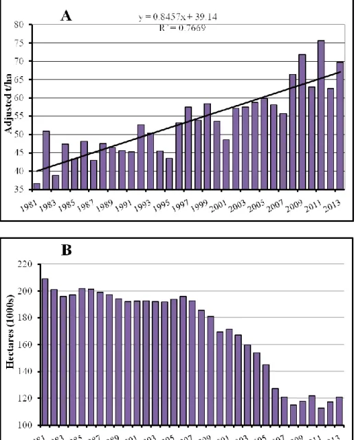
Figure 1.1: Average sugar beet yield (from British Sugar data) from 1981 to 2013 (A), and the UK area harvested (B) . ... 7

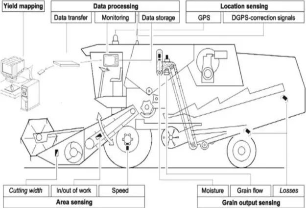
Figure 1.2: Illustration of the sensing systems in combine harvester. ... 26

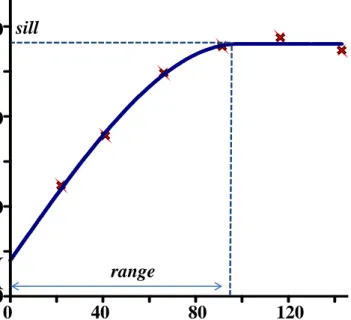
Figure 1.3: The experimental variogram of the data of crop canopy cover in July 2012 in White Path field presented as an example of a typical shape of variogram. ... 32

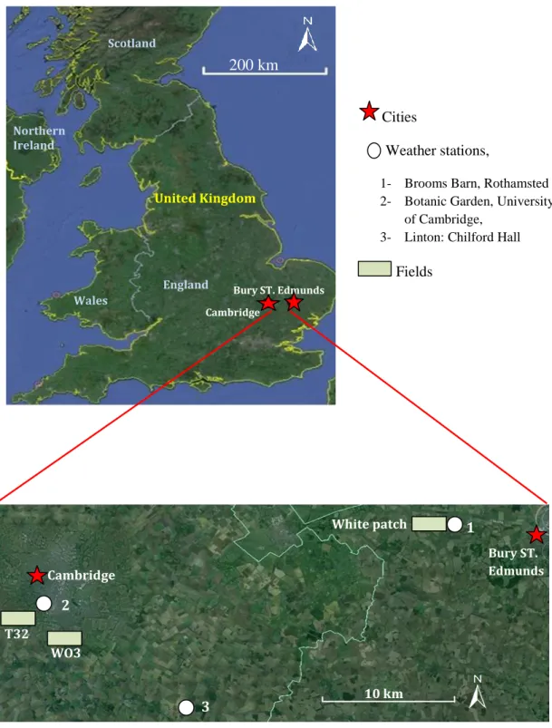
Figure 2.1: Study sites and the locations of the fields and weather stations overlaid on Google Earth map in 8th of September 2014. ... 78

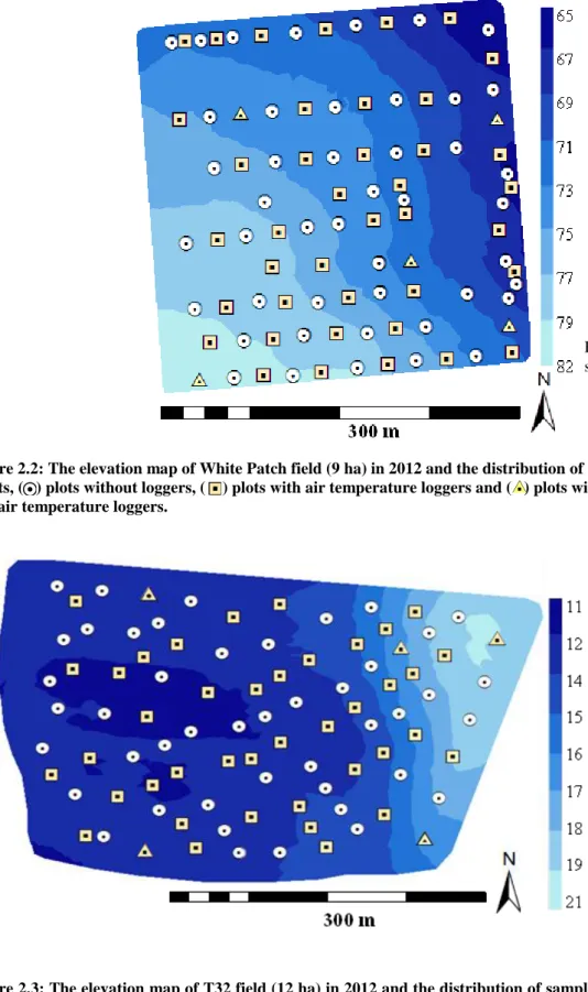
Figure 2.2: The elevation map of White Patch field (9 ha) in 2012 and the distribution of sampling points. ... 81

Figure 2.3: The elevation map of T32 field (12 ha) in 2012 and the distribution of sampling points. ... 81

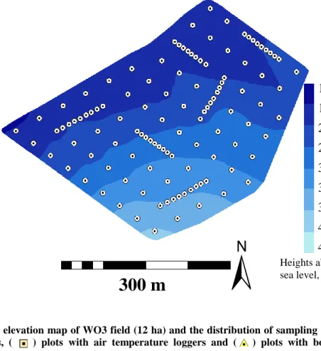
Figure 2.4: The elevation map of WO3 field (12 ha) and the distribution of sampling points. ... 82

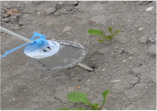
Figure 2.5: The polystyrene cups covered with aluminium foil to protect the loggers. ... 87

Figure 2.6: The monthly average, minimum and maximum temperatures ... 98

Figure 2.7: The left hand side is the soil temperature (degrees Celsius) to 10 cm depth respectively at Brooms Barn and Trumpington in 2012 and Shelford in 2013; the right hand side is the monthly amount of precipitation (mm)). ... 99

Figure 2.8: Picture (A) a patch from White Patch field which was almost free from weeds and picture (B) is another patch of the same field with high weed density. ... 106

xii

Figure 3.1: The experimental variograms and fitted models for the studied environmental variables in White Patch Field in 2012.. ... 116

Figure 3.2: Interpolation maps for the studied environmental variables in White Patch Field in 2012. ... 118

Figure 3.3: The maps of average monthly mean canopy temperature (°C) based on daily records in White Patch field in 2012 season ... 120

Figure 3.4: The experimental variograms and fitted models for the studied environmental variables in 2012in T32 Field in 2012.. ... 124

Figure 3.5: Interpolation maps for the studied environmental variables in T32 filed in 2012. ... 125

Figure 3.6: The maps of average monthly mean canopy temperature (°C) based on daily records in T32 field in 2012 season ... 127

Figure 3.7: The experimental variograms and fitted models for the studied environmental variables in WO3 Field in 2013. ... 131

Figure 3.8: Interpolation maps for the studied environmental variables in WO3 field in 2013. ... 132

Figure 3.9: The maps of average monthly mean canopy temperature (°C) based on daily records in WO3 field in 2013 season ... 134

Figure 4.1: The experimental variograms for the crop growth parameters, yield and quality of sugar beet in White Patch field in 2012. ... 149

Figure 4.2: The experimental variograms for the crop growth parameters, yield and quality of sugar beet in T32 field in 2012. ... 150

xiii

Figure 4.3: The experimental variograms for the crop growth parameters, yield and quality of sugar beet in WO3 field in 2013 ... 151

Figure 4.4: Interpolation maps for the crop growth parameters, yield and quality of sugar beet in White Patch field in 2012. ... 156

Figure 4.5: Interpolation maps for the crop growth parameters, yield and quality of sugar beet in T32 field in 2012. ... 157

Figure 4.6: Interpolation maps for the crop growth parameters, yield and quality of sugar beet in WO3 field in 2013 ... 158

Figure 4.7: The interpolation maps for the yields of (A) wheat in 2011, (B) sugar in 2012, and the average relative yield of both crops (C) in T32 field. ... 165

Figure 4.8: The interpolation maps for WO3 for yields of (A) Oilseed rape in 2011, (B) wheat in 2012, (C) sugar in 2013, average relative yield (D), the temporal variance (E), and management zones. ... 166

Figure 4.9: Ordination biplots based on redundancy analysis of the sugar beet yield and quality data with environmental variables, crop growth parameters and weed density in White Patch field in 2012 ... 170

Figure 4.10: Ordination biplots based on redundancy analysis of the sugar beet yield and quality data with environmental variables, crop growth parameters and weed density in T32 field in 2012. ... 172

Figure 4.11: Ordination biplots based on redundancy analysis of the sugar beet yield and quality data with environmental variables, crop growth parameters and weed density in WO3 field in 2013. ... 174

xiv

Figure 4.12: Ordination biplot based on redundancy analysis of the normalized and combined root yield for all field and quality data with combined environmental variables crop, growth parameters, and weed density ... 176

Figure 4.13: Ordination biplot based on redundancy analysis of the normalized and combined crop canopy cover in June for all field and quality data with combined environmental variables used as explanatory variables. ... 177

Figure 5.1: Components and controlling environmental variables in the Broom’s Barn sugar beet growth simulation model. ... 189

Figure 5.2: Images of the minimum (A, D, G), mean (B, E, H) and maximum (C, F, I) canopy cover in the three fields ... 199

Figure 5.3: The relationships between observed and simulated crop canopy covers in June before (A-C) and after (D-F) adjusting the sowing date in the three fields ... 200

Figure 5.4: The relationships between observed sugar yield and plant population (A-C) and weed density (D-F) in the three fields ... 201

Figure 5.5: The linear relationships between observed and simulated sugar yield in White Patch field in 2012.. ... 209

Figure 5.6: The linear relationships between observed and simulated sugar yield in T32 field in 2012. ... 210

Figure 5.7: The linear relationships between observed and simulated sugar yield in WO3 field in 2013.. ... 211

Figure 5.8: The interpolation maps for the observed and simulated sugar yield t/ha and the relative yield gap based on adjusted and unadjusted sowing dates in White Patch field in 2012.. ... 214

xv

Figure 5.9: The interpolation maps for the observed and simulated sugar yield t/ha and the relative yield gap based on adjusted and unadjusted sowing dates in T32 field in 2012. ... 215

Figure 5.10: interpolation maps for the observed and simulated sugar yield t/ha and the relative yield gap based on adjusted and unadjusted sowing dates in WO3 field in 2013.. ... 216

Figure 6.1: The Kriging maps of relative yield of (A) sugar beet with previous winter wheat crop in T32, and (C) sugar beet with previous winter wheat and oilseed rape in WO3, and the Kriged map of yield gap between the simulated and observed sugar yield (B) in T32 and (D) in WO3). ... 240

xvi

List of Tables:

Table 1.1: The areas planted with sugar beet (1000 ha), total root production (1000 tonnes) and root yield (tonnes/ha) in the world and the ten largest sugar beet producers in Europe 2010. ... 6

Table 1.2: The required accuracies of GPS signals for agricultural application ... 15

Table 2.1: The area, variety planted, number of samples, date of planting and harvesting, previous crop and some field operation during the growing season at each field. 79

Table 3.1: Results of statistical and geostatistical analysis of some soil physical and chemical attributes in White Patch field in 2012. ... 115

Table 3.2: The summary statistics of average mean, minimum and maximum canopy temperature °C at different stages in White Patch field in 2012. ... 120

Table 3.3: Results of statistical and geostatistical analysis of some soil physical and chemical attributes at T32 field in 2012. ... 122

Table 3.4: The summary statistics of average mean, minimum and maximum canopy temperature °C at different stages in T32 field in 2012. ... 127

Table 3.5: Results of statistical and geostatistical analysis of some soil physical and chemical attributes in WO3 field in 2012 ... 129

Table 3.6: The summary statistics of average mean, minimum and maximum canopy temperature °C at different stages in WO3 Field in 2013. ... 134

Table 3.7: Correlation coefficients between (A) soil properties and, (B) between soil and air temperature °C and soil moisture in White Patch in 2012 ... 137

xvii

Table 3.8: Correlation coefficients between (A) soil properties and, (B) between soil and air temperature °C and soil moisture in T32 in 2012 ... 138

Table 3.9: Correlation coefficients between some studied soil properties in WO3 filed in 2013 ... 139

Table 4.1: Summary statistics of sugar beet growth, yield and quality in White Patch in 2012. ... 143

Table 4.2: Summary statistics of sugar beet growth, yield and quality in T32 in 2012. .. 144

Table 4.3: Summary statistics of sugar beet growth, yield and quality in WO3 in 2013. 144

Table 4.4. Geostatistical analysis of sugar beet growth, yield and quality in White Patch in 2012. ... 147

Table 4.5: Geostatistical analysis of sugar beet growth, yield and quality in T32 in 2012. ... 147

Table 4.6: Geostatistical analysis of sugar beet growth, yield and quality in WO3 in 2013. ... 148

Table 4.7: Correlation coefficients between sugar beet yield and quality, and studied physical and biological variables in White Patch in 2012 ... 159

Table 4.8: Correlation coefficients between sugar beet yield and quality, and studied physical and biological variables in T32 field in 2012 ... 160

Table 4.9: Correlation coefficients between sugar beet yield and quality, and studied physical and biological variables in WO3 in 2013 ... 161

Table 4.10: The summary statistics and correlation coefficients for sugar yield, previous crops (winter wheat and oilseed rape) and average standardized yield.. ... 164

xviii

Table 4.11: The summary statistics of four constrained axes of the redundancy analysis for the sugar beet crop in each field separately and for combined analysis including all three fields.. ... 168

Table 4.12: The percentage of variation accounted for by the explanatory variables and its significance (P values) based on redundancy analysis for the sugar beet crop ... 169

Table 5.1: The main components and variables of Broom’s Barn sugar beet growth model

and their mathematical equations ... 190

Table 5.2: Specifications and values of some parameters and variables used in the original Broom’s Barn sugar beet growth model and their mathematical equations). ... 191

Table 5.3: Summary statistics of observed and simulated sugar yields t/ha and the relative yield gap between observed and simulated sugar yield. ... 203

Table 5.4: Correlation coefficients and the parameters of linear regression between observed and simulated sugar yield t/ha, and adjusted simulated yield. ... 204

Table 5.5: The significance (P values) of the correlation coefficients between observed and simulated sugar yield: ... 207

xix

List of Appendices:

Appendix 1: The maps of some soil properties of the fields………266

Appendix 1- 1: The map of main soil types at White Patch field in 2012...266

Appendix 1- 2: The map of main soil nutrients and pH at T32 field in 2011 ………....267

Appendix 1- 3: The map of main soil nutrients and pH at WO3 field in 2013……...268

Appendix 2: The maps of crops preceding sugar beet crop ………...269

Appendix 2- 1: The yield map of winter wheat in T32 in 2011………...269

Appendix 2- 2: The yield map of winter wheat in WO3 in 2012 ………..270

Appendix 3: Conversion of actual beet tonnage into adjusted beet tonnage ……..271

Appendix 4: Identifying the yield (t/ha) of previous crop (winter wheat) in the plots where the sugar beet measurements were taken in T3 field………...272

Appendix 5: The histograms of original and transformed data…………..…....…..273

Appendix 5- 1: In White Patch field………...…...………...273

Appendix 5- 2: In T32 field……….274

xx

Appendix 6: The experimental variogram fitted with different models……….276

Appendix 7: The model parameters and the excremental variograms for the simulated yields in all three fields……….…………277

Appendix 7.1: The model parameters for the variograms of simulated yields in the three fields………....277

Appendix 7.2: The experimental variograms of simulated yields in White patch field………278

Appendix 7.3: The experimental variograms of simulated yields in T32 field……….……279

Appendix 7.4: The experimental variograms of simulated yields in WO3 field………..280

Appendices 8: The interpolation maps for the adjusted simulated yields and yield gaps………..281

Appendix 8- 1: In White Patch in 2012………...281

Appendix 8- 2: In T32 in 2012………..………...282

Appendix 8- 3: In WO3 in 2013………...283

Appendix 9: The correlation coefficients and their significance against zero for the studied variables. ………...284

Appendix 9- 1: Correlation coefficients between the studied variables in White Patc…284 Appendix 9- 2: Test the significance of the correlations against zero in White Patch…287 Appendix 9- 3: Correlation coefficients between the studied variables in T32…….…....290

xxi

Appendix 9- 4: Test the significance of the correlations against zero in T32………...293 Appendix 9- 5: Correlation coefficients between the studied variables in WO3….……..296 Appendix 9- 6: Test the significance of the correlations against zero in WO3…………299

xxii

List of Abbreviations:

%- Percentage

£- Great Britain pound

γ(h)- Semivariance µS- Microsiemens °C- Degree Celsius

a - Range of spatial dependency identified by the variogram BBRO- British Beet Research Organization

BLUP- Linear unbiased predictor C1- Sill variance

C0- Nugget variance

C0/(C1+ C0)- Nugget to sill ratio

CC- Crop canopy cover

CEDA- Centre for Environmental Data Archival CGR- Relative canopy growth rate

CV- Coefficient of variation d- Day

DEM- Digital elevation model

dGPS- Differential global positioning system EC- Electrical Conductivity

xxiii ET- Evapotranspiration

GIS- Geographic information system GPS - Global positioning system h- Lag distance

ha- Hectare

IDW- Inverse Distance Methods K- Potassium

LAI- leaf area index LOI- Loss-On-Ignition m- Metre

MaxT- Maximum temperature Mg- Magnesium

MinT- Minimum temperature MoM- Methods of moments MZ- Management zones N- Nitrogen

NDVI- Normalized differential vegetation index OK- Ordinary kriging

P- Level of significant (Probability of error) P- Phosphorus

xxiv PAR- Photosynthetically active radiation pH- Soil acidity

PP- Plant population r- Correlation coefficient

R2- Regression coefficient of determination RDA- Redundancy analysis

RI- Relative improvement index RMS- Residual Mean Square

RMEL- Residual Maximum Likelihood RMS- Residual mean of Square

RTK GPS- Real Time Kinematic Global Positioning System SD- Standard deviation

SMC- Soil moisture content SOM- Organic matter

SRI- Solar radiation interception T- Mean temperature

t- Tonne

VRA- Variable rate application UK- United Kingdom

1

1. Chapter One: Introduction and Literature Review.

1.1 Introduction:

A major concern of agriculturists has been devoted recently to increase land productivity in order to meet the world food demand for increasing world population, which is expected to reach 9 billion by 2050 (Pati et al., 2011, Oliver et al., 2013). However, the environment and the costs of production are another growing concern; therefore they should be considered when increasing the land productivity. For this purpose, a precise investigation of crop environment such as soil properties and micro-climate which can differ significantly in spatial and temporal scales is required (Heege, 2013). Especially for some crops such as sugar beet, as the world demand of sugar is expected to reach 140 million tons per year (Draycott, 2008, Samson-Bręk, 2010). This thesis considers modelling and mapping the within field variability in sugar beet yield and aims to identify the main driving variables potentially causing within-field variation. Therefore most of the environmental factors that have a potential influence on sugar beet yield have been investigated as well as the interaction between these variables. In addition, the possibility of anticipating the non-uniformity in final economic yield early in the growing season or from yield information of the previous crop has also been examined.

Conventionally, most commercial agricultural fields are generally managed with uniform application of tillage and agronomic inputs which can adversely affect the environment, increase the costs of production and waste natural resources (Montanari et al., 2012).

2

However, it is well-known that there is within-field variability at different spatial and temporal scales (Webster and Oliver, 2007), which affects crop development and is reflected in the non-uniformity in yield (Heege, 2013). This variability could be managed by applying the right amount of inputs in the right place at the right time in order to optimize benefits, increase sustainability and decrease adverse environmental impacts (Mondal et al., 2011, Najafabadi et al., 2011, Diacono et al., 2013). Factors such as soil fertility, pH, water deficit, weeds, pests and diseases could be managed spatially, while others such as soil texture, topography and climate conditions cannot (Sadler et al., 1998, Frogbrook et al., 2002). Some of these variables are visible and can be seen easily from ground based, airborne and satellite imagery, while others such as temperature and soil chemical composition are difficult to see and require direct measurement and soil analysis (Webster and Oliver, 2007).

In England, recent studies predict that sugar yield is likely to increase in the future by about 0.5-1.5 t/ha in sandy soils and 2 t/ha in loamy soils by 2050 and 4 t/ha by 2080, due to the advances in plant breeding and agronomic progress (Richter et al., 2006), but the variation in sugar beet yield due to weather condition is more likely to increase in un-irrigated areas (Freckleton et al., 1999), because in these areas the effect of water stress is additional to the effect of temperature and solar radiation (Jaggard et al., 2007). The variation within regions is expected to be higher than the variation between regions due to the variability in soil properties (Richter et al., 2006). Therefore identifying spatial variation in environmental conditions could provide important information for water and nutrient management and fertilizer application in sugar beet fields (Sağlam et al., 2011, Montanari et al., 2012) and

3

consequently optimize benefits, increase sustainability and decrease adverse environmental impact. For this purpose various studies have been conducted to address the causes of within-field variation in crop yield. Some of these studies have attributed this variation to soil texture and soil organic matter (Taylor et al., 2003, Shaner et al., 2008, Karaman et al., 2009a), soil nutrients (Vanek et al., 2008, Rodriguez-Moreno et al., 2014), which have a significant effect on crop yield, to the variation in soil available water in relation soil types, field topography and the proportion of sand and stones (Vanek et al., 2008, Zhang et al., 2011a, Korres et al., 2013), to management practice (Taylor et al., 2003) or to some other driving variables such as the diffusion of water and nutrient which are quite complex and are difficult to investigate (Lark, 2012). However, only a few studies have considered the spatial variability in sugar beet fields and most of these studies considered a single environmental variable such as soil organic matter (Karaman et al., 2009a), soil nutrient (Franzen, 2004, Karaman et al., 2009b), soil moisture content (Zhang et al., 2007, Zhang et al., 2011a), or diseases and nematodes (Reynolds, 2010, Hbirkou et al., 2011). In addition, the spatial relationship between the studied environmental variable and sugar beet growth or yield was not examined, thus the studied variable might not be limiting the yield. The within-field variation could be due to the combined influence of different soil and micro-climate factors and it is quite difficult to isolate the effect of a single environmental factor. These factors can be laid into four main groups as follows: soil texture which can affect soil moisture and soil structure, topography in relation to micro-environment, soil nutrients and, weeds, diseases and pests (Godwin and Miller, 2003). Therefore, detecting the spatial variability in sugar beet yield in relation to the independent and combined effects of

4

different environmental variables is required and likely to be important to achieve the improvement in sugar beet growth and yield.

In addition, crop stress is usually observed and treated when it becomes visible; by which time the damage has already occurred and the crop may not recover fully (Bouma, 1997). For example the appearance of Rhizoctonia crown and root rot in sugar beet fields can be revealed by aerial photographs, but only when it is moderately to severely infected (Reynolds, 2010), when chemical treatments might not reduce its effect on final yield. Also the effect of water stress on the crop is usually seen only when the crop starts wilting (Zhang et al., 2011a), and it has been found that exposing a sugar beet crop to water stress in early growth stages even for short periods can significantly reduce the final sugar yield (Yang et al., 2007). Therefore, anticipating the spatial variability in sugar beet yield early in the growing season could help the farmer to take precautions to avoid or mitigate the damage. Furthermore, simulating within-field variability in sugar beet yield using the crop preceding sugar beet in the rotation as a predictor also needs to be assessed, since this might help to reveal expected variation in sugar beet yield and anticipate the spatial and temporal variation over many years. Moreover, modelling the growth of sugar beet crop based on the spatial variability in micro- environmental conditions has not been taken into consideration yet as the current models are usually applied only on a regional basis.

5

1.2 Sugar beet crop:

Sugar beet along with sugar cane are the two main global sources of sucrose, for which there is a large global market of high economic importance. Sugar beet is considered as a new crop developed from white fodder beet in the 18thcentury, and producing the sugar from sugar beet was one of the important agricultural achievements in the 19th century (Draycott, 2008). It is now grown under a wide range of temperate weather conditions; it is grown as a summer crop in the northern parts of temperate areas and as a winter crop in southern parts of these areas (Draycott, 2008). In most of Europe sugar beet is an un-irrigated crop, it is usually sown in spring and the sugar accumulation starts early in the growing season. The long vegetative growth period increases the sugar percentage in the root due to extending the sugar accumulation period (Jaggard et al., 2009). For sugar production the growing season in these areas is usually between 170-200 days. Mild weather during the growing season can significantly increase the root yield, and low temperatures near the end of the season can enhance sucrose accumulation (Samson-Bręk, 2010).

Sugar beet currently supplies approximately 40 million tonnes of sucrose annually which represents 30% of global demand of sucrose, approximately 75% of this amount being produced by Europe and United States, while sugar beet production is not significant in central Asia and Caucasus countries, due to unsuitability of weather conditions (FAO, 2012). The top ten sugar beet producers in Europe with the average area planted by sugar beet, total production, the yield per hectare and the percent global share in 2010 are listed in

6

Table 1.1 (FAO, 2012). These countries produce more than 60% of sugar and the top country is France which produces approximately 14% of world production of sugar beet.

Table 1.1: The areas planted with sugar beet (1000 ha), total root production (1000 tonnes) and root yield (tonnes/ha) in the world and the ten largest sugar beet producers in Europe 2010 (FAO, 2012).

Country Area planted

(1000 ha) Roots production (1000 tonnes) Roots yield (tonnes /ha) Percent global share World 4676 228452 48.86 - France 383 31910 83.32 13.97 Germany 367 23858 65.01 10.44 Russia 924 22256 24.09 9.74 Turkey 329 17942 54.53 7.85 Ukraine 492 13749 27.95 6.02 Poland 200 9823 49.12 4.30 United Kingdom 122 7686 63.01 3.36 Netherlands 71 5280 74.37 2.31 Belgium 59 4465 75.68 1.95 Italy 63 3550 56.35 1.55

In 2010-2011 sugar beet occupied approximately 3% of the UK arable land, and this produced around 1.3 million tonnes of sugar with an average root yield of 75 t/ha (Limb, 2014). Sugar beet yield (t/ha) in UK has significantly increased from the period between 1981 and 2013 (Fig. 1.1a), the significant increase in yield was associated with significant declines in the area planted to sugar beet (Fig. 1.1b) and the number of growers (Limb, 2014). Similar trends were also observed in France for the period between 1980 and 2010, but was associated with decrease in sugar beet prices (Boizard et al., 2012). This could be due to the changes in the EU support polices, which reduced sugar beet production in Europe by 20% and the area harvested also reduced to less than 1% of total world arable land in 2009 (FAO, 2012). The recent increase in sugar yield in the UK, which is estimated

7

to be around 0.111 t/ha/year on UK tonnes and about 0.204 t/ha/year in the official varieties trials, is due to the improvements in sugar beet varieties and agronomic practice, in addition to the ability of sugar beet plant to adapt to the recent weather conditions (Jaggard et al., 2007, Jaggard et al., 2009).

Figure 1.1: Average sugar beet yield (from British Sugar data) from 1981 to 2013 (A), and the UK area harvested (B) (Limb, 2014).

8

The role of plant breeding appears to be greater than agronomic practices because improved varieties have significantly increased root sugar content from 12% to 20% with improvement in yield and other chemical content as well as increasing sugar beet resistance to diseases and pests. The amount of white sugar produced by sugar beet has therefore increased (Draycott, 2008). Conversely, changes in some other agronomic processes such as extending the period of crop processing by storing beets after harvest and reducing the irrigated areas have reduced sugar beet yield (Jaggard et al., 2009). Despite the significant increases in sugar beet yield per ha over last four decades, sugar beet growers face various challenges and the recent changes in weather conditions are considered to be a major challenge to sugar beet production in the UK. Some of the environmental factors that affect sugar beet growth are outside the grower’s control, while others such as plant nutrients can be added in different ways by growers and achieve significant benefits (Draycott and Christenson, 2003). Perhaps the most important factor in Europe is soil moisture, since most sugar beet is rain-fed. In addition sugar beet growers regularly suffer from uneven plant populations due to the lack or delay of irrigation (Sadeghian and Yavari, 2004). On the other hand, in the Mediterranean region the effect of temperature on sugar beet yield is considered to be greater than the effect of drought, due to the increase in the evapotranspiration rate (Abd-El-Motagally, 2004). The effect of some of these factors on sugar beet growth and production might occur at different spatial and temporal scales. Investigating the spatial variation in sugar beet yield and its relation

9

to the soil properties and micro-climate condition is important to maximise the yield, reduce the costs of production and adverse environmental impact.

1.3 Precision agriculture (PA):

Precision agriculture is a modern technique, growing rapidly in western countries. Its scientific goal is to develop a farm’s management with the potential of increasing the land productivity based on precise information about spatial variability in environmental attributes that potentially cause yield variation (Mondal et al., 2011). Based on this approach the fertilizers, seeds and pesticides can be customized to specific zones rather than uniformly applied across a field by increasing the amount of the inputs where they are required and decreasing where not (Bouma, 1997, Rains and Thomas, 2009, Pati et al., 2011, Oliver etal., 2013). Conventionally, most of the recommendations about agricultural inputs such as fertilizer and pesticides were derived for uniform application. However, the environmental variables such as solar radiation, available water, soil properties and topography are never uniform even within the field scale (Heege, 2013). As a consequence of uniform application, parts of the field will receive less inputs than required, which might limit the yield, while other parts might receive more than they need, which will waste the natural resources and may adversely affect the environment such as by leaching nutrient and pesticide to the ground water and contaminating it (Oliver et al., 2013). This has prompted researchers and farmers to adopt precision agriculture, so that the spatial variation in yield and associated environmental variables can be identified and managed by variable rate application of the inputs, which can enhance the yield uniformity and reduce

10

the adverse environmental impact (Auernhammer, 2001, Najafabadi et al., 2011, Oliver et al., 2013). Precision agriculture (PA) in relation to climate and soil conditions is expected to have an increasingly important role during the 21st century, which needs the combination of spatial technologies such as global positioning system (GPS), geographic information system (GIS) and remote sensing, as well as the possibility of analysing the spatial relationship between mapped variables in order to conduct management practice according to the spatial and temporal variability across the natural and agricultural landscapes (Berry et al., 2003, Najafabadi et al., 2011, Clay, 2011).

Precision agriculture has been widely examined for its profitably and accuracy over the last decade and promising results have been achieved. The economic advantages of variable rate nitrogen fertilization in sugar beet fields were estimated to be about US$50 ha-1 for grid based sampling and about US$ 113ha-1 for zone based sampling compared to uniform application (Franzen, 2004). The average increase in gross incomes, which means the advantages of maximizing the yield with minimizing the inputs, is estimated to be around US$ 150 ha-1 in maize field and US $51 ha-1 in soybean by applying precision agriculture (Amado and Santi, 2011). In addition the amount of herbicides applied, costs and required working hours were significantly lower compared to uniform application (Pedersen et al., 2005, Mohammadzamani et al., 2009).

Due to the advances in the spatial technologies that have an important role in the adoption of precision agriculture, it becomes possible and easy to collect information for mapping the yield of many crops. Remote sensing can provide reliable information about the land cover, land use changes and plant growth (Delegido et al., 2011). For example it can

11

provide an accurate map of leaf area index or crop cover which might be correlated with the within field variation in yield (Martinez et al., 2010). In addition an accurate yield map for combinable crops can be produced cheaply by the combine harvester during the harvest (Griffin, 2010, Heege, 2013). However the map of yield or any other crop growth parameters during growing season provided by these techniques is not sufficient for implementation of precision agriculture, because it does not map the actual stress, but it usually represents the plant response to the stress, and different environmental variables can cause a similar pattern of stress (Jones and Schofield, 2008). Therefore an accurate map of the main environmental variables that have a potential causal influence on yield variation is also required. For some variables such as soil properties and water status, this map cannot be provided by the combine harvester and will not be accurate enough if it provided by remote sensing. For example the soil available water can only be detected by traditional remote sensing techniques for shallow depths, which is not useful to detect the water status for root crops such as sugar beet that absorb the water from 100 cm (Rains and Thomas, 2009). Therefore the field needs to be sampled and all the data should be based on these samples. On the other hand sampling the field intensively to obtain an accurate map for management is difficult and expensive (Webster and Lark, 2012), and the measurements will just represent the locations at which the samples have been taken (Scannavino et al., 2011). Using geostatistical methods of interpolation such as Kriging that can predict the value of the property in unsampled locations (Oliver, 2010), but the sampling protocol to obtain the best prediction is still controversial (Kerry, 2003). Therefore precision agriculture needs a combined approach between different techniques to produce an accurate map with reducing the sampling efforts (Kerry et al., 2010),

12

because each of these techniques has its limitations if it is applied separately, and combining two or more of these technologies will be complementary to each other, and this will broaden the scope for which they are applicable (Gao, 2002). It has become evident that promising results can be obtained by integrating remote sensing techniques with soil map and crop measurement (Oliver et al., 2013). For example using remote sensing techniques for mapping an environmental property can be associated with an error that needs to be statistically quantified by ground truthing (Rocchini et al., 2013). The information about spatial variation provided by remote sensing, electrical conductivity scanning and yield mapping by a combine harvester is useful not only for detecting the stress in crop growth or to identify soil types, it is also needed to identify management zones for variable rate applications and to guide sampling schemes for geostatistical analysis (Bouma, 1997, Kerry and Oliver, 2007a, Kerry et al., 2010). Using the auxiliary data provided by these techniques as a covariate can enhance prediction of spatial variability in soil properties (Minasny and McBratney, 2007), and it can be a useful to monitor the patterns of variation over time and link it with ground truth data of the soil properties or micro-climate for precision agriculture applications in the following crop in the rotation.

1.3.1 Precision agriculture tools:

As the implementation of precision agriculture requires the adoption of spatial technologies such as GPS, GIS and remote sensing and methods of mapping the spatial patterns, its application has now become more promising as a result of the progress in these techniques.

13

The availability of these technologies provides an easy way to gather important information about crops and environment. Each of these technologies is described in the following sections.

1.3.1.1 Global Positioning System (GPS):

GPS, was used initially as a navigation system developed by the United States military to identify the position on the earth and it is based on 24 satellites distributed in the earth’s orbit (Rains and Thomas, 2009, Chu Su, 2011). The main merits of GPS are that the signal is free and can be used at any time and it works without the effect of weather. Therefore its application has become more popular world-wide and the instruments can identify each satellite’s position by receiving its broadcasted signal to provide a triangulated georeference (Auernhammer, 1999, Shanwad et al., 2002). Accuracy has now increased from about 100 m to about 10cm (Gavric and Martinov, 2007). As a result of the development of GPS and its integration with other technologies such as remote sensing and GIS, the spatial data about crop condition can be collected easily and efficiently and it can be used by the farmer or their advisors for managing their fields site-specifically (Gao, 2002, Corwin and Lesch, 2005, Aziz et al., 2009). The accurate data required for precision agriculture cannot be provided by the raw GPS; therefore it requires an additional signal from known reference to obtain desirable accuracy such as differential GPS that use the additional signal (Rains and Thomas, 2009). In addition to differential GPS, real time kinematic global positioning system (RTK GPS), which is the most accurate generation of GPS is available for agricultural purposes that need more accuracy. The required accuracies of GPS for various agriculture applications are given in Table 1.2.

14

1.3.1.1.1 Differential Global Positioning System (dGPS):

Differential global positioning system (dGPS) is an enhancement to global positioning system (GPS) which improved the position accuracy of GPS from 15 m to 10 cm in case of the best implementation. In 1987 the U.S. Coast Guard Research and Development (R & D) Centre announced that the accuracy of GPS has been improved significantly by using dGPS correction broadcast to local user equipment within the coverage area of the correction broadcast (Schlechte and Officer, 1994). It operates based on triangulating the signal released from the satellites and it can receive and combined real time correction data provided by the coast guard GPS correction system which made significant improvement in the accuracy of GPS and it can provide resolution within one meter (Nagchaudhuri et al., 2005). This resolution is sufficient to determine the position within agriculture fields for different applications and most agricultural equipment used for precision agriculture are provided with this kind of GPS (Rains and Thomas, 2009), and it has been widely used for yield mapping, yield monitoring, soil sampling which are important for describing the spatial variation (Chu Su, 2011). One of the main advantages of using dGPS is that it can solve the digital noise problems with some specifications, but the main drawback of its application in agriculture is that it increases the cost of operation (Mondal et al., 2011).

1.3.1.1.2 Real Time Kinematic Positioning System (RTK GPS):

RTK GPS is one of the most accurate kinds of GPS; it can provide the position information within centimetres accuracy (Mondal et al., 2011). RTK GPS commercially became

15

available in 1992 with measurement capabilities within 1 to 4 cm accuracy (Buick, 2006). Due to its sensitivity of use (horizontal ±2 cm, vertical ±4 cm), and being easy to be applied, it has become more preferable and most widely used in many studies especially mapping environmental variables and mining survey (Yılmaz et al., 2006). It also can be used effectively for topographic mapping and it has 5cm accuracy for elevation, due to its capability to extract extra information by assessing the carrier of the GPS signal (Sudduth, 1998). However, it is more expensive than some other precision agriculture equipment such as machine vision guidance system (Slaughter et al., 2008). It can provides autonomous systems with better results for robotic weed control and it can be used for more accurate variable rate application, but it is still relatively expensive and it increases the costs for autonomous systems (Pedersen et al., 2005, Chu Su, 2011).

Table 1.2: The required accuracies of GPS signals for agricultural application (Auernhammer, 1999).

Required accuracy Task Examples

± 10 m Navigation _ Targeting of fields (machinery ring, contractor)

Targeting of storage area (forestry)

±1m Job execution

Information Documentation

 Local field operations with yield monitoring, fertilizing, plant protection, soil sampling, action in protected areas

 Automated data acquisition

±10 cm Vehicle guidance _ Gap and overlay control (fertilizing, spraying) Grain combining

±1cm Implement (tool)

16

1.3.1.2 Geographic Information System (GIS):

According to the National Centre of Geographic Information and Analysis (NCGIA), GIS can be defined as “a system of hardware, software and procedures to facilitate the management, manipulation, analysis modelling, representation and display of georeferenced data to solve complex problems regarding planning and management of resources” (Mutluoglu and Ceylan, 2009). The main feature of GIS is that it can integrate, analyse, and model the data from different sources depending on its powerful analytical functionality (Gao, 2002). As most of the environmental variables that relate to agriculture have some form of spatial variation, the adaption of GIS software in precision agriculture provides a great opportunity to visualize these data especially if that might be difficult to present in other ways (Pierce and Clay, 2007). For example, many maps of different variables or different years can be combined to describe the interaction between them and detect the variation patterns over many years (Blackmore, 2003). The integration of GIS with other techniques is important for precision agriculture (Gao, 2002), and the combination of GIS and GPS is most important for creating a map that can show the farmer which parts of the field need more inputs than others (Bullock et al., 2002, Nutter et al., 2011). In addition, the advanced generation of GIS is provided by the geostatistical analyst toolbar, which has filled the gap between GIS and geostatistics. This is useful to quantify the quality of the surface map by estimating the statistical errors associated with prediction (Johnston et al., 2001, Shahbazi et al., 2013). However, using GIS is still unreliable for weed mapping, as the different maps of weed distribution produced by GIS based on different sampling schemes and starting points were not related to each other (Backes and Plümer, 2003). This might be a serious issue especially if the map has over or

17

underestimated the actual distribution of weeds, because it will waste the chemical resources and may affect the long term spreading of specific weeds (Backes and Plümer, 2003).

1.3.1.3 Remote sensing:

Remote sensing can provide multispectral information based on emitted radiation from the target point, which could be a bare soil or vegetative cover as a series of narrow wavelength across a geographical location (Diacono et al., 2013, Meroni et al., 2009). This information can then be utilized to describe the spatial variation in biotic and abiotic variables of the ecosystem such as land cover, land use, vegetation and soil properties, as well as detecting the changing patterns over time (Rocchini et al., 2013). The combination of remote sensing with GPS and GIS increases its capability to detect and map the spatial and temporal variability in crop growth and soil properties and has become an important tool for precision agriculture (Sivarajan, 2011). In addition, it can provide a good explanation of the relationship between crop biophysical data or vegetative indices such as vegetation development, photosynthetic activity, biomass accumulation, leaf area index (LAI), and crop evapotranspiration (ET), with crop production (Jayanthi, 2003). Remote sensing technologies involve different systems such as satellite-based systems (satellite images), airborne-based systems (aerial photography) and ground-based systems (e.g. with vehicle mounted camera). The adaptation of remote sensing imagery for in field decision making has some limitations such as the high cost, non-availability in real time and it requires high scientific knowledge to analyse and interpret data. Providing low or no-cost value-added

18

products that can be interpreted easily is one of the ways to face these challenges (Zhang et al., 2010a). The main factor affecting the reliability of remote sensing is that it describes the gradual variation in a property as a set of discrete non-interacting classes which might lead to loss of some information when classifying and processing the images (Rocchini et al., 2013).

1.3.1.3.1 Satellite images:

Most kinds of satellite images are originally multispectral, but they have lower spatial resolution compared to other kinds of remote sensing technologies (Reynolds, 2010). Satellite imaging has become a useful tool in precision agriculture. It has many advantages such as that it can capture large areas, the possibility of analysing a single image, it can process rapidly, accurate information is available using different wavebands, the availability of previous images for comparison and the data can be recorded without any administrative limitation by national government (Sivarajan, 2011). The most important source for precision agriculture is QuickBird, due to its high resolution especially the red (630 to 690 nm) and near infrared portions of the spectrum (760 to 900 nm) (Laudien et al., 2004). This technique could be used to map leaf area index, which is important for decision making for irrigation and canopy management (Johnson et al., 2003, Silva et al., 2007). For example Franzen (2004) divided satellite images of a sugar beet field into different green and yellow areas to develop management zones for variable nitrogen fertilization. The same approach was followed by the farmers in Red River Valley in Minnesota. They used Landsat TM derived normalized differential vegetation index (NDVI) of a sugar beet field

19

to create zones to estimate site-specific nitrogen credits, the higher dark green area indicated higher N, which needed less fertilizer for the following crops in these zones and the farmer saved $30 per hectare (Zhang et al., 2010a). To identify the optimal number of management zones automatically and delineate them using satellite imagery, the zones based on satellite image with NDVI value were significantly correlated with soil organic matter concentration (Zhang et al., 2010b). The NDVI map provided by satellite images can also be used for detecting the damage caused by diseases (Mondal et al., 2011), and thus it has successfully detected the area of sugar beet field affected by Rhizoctonia crown and root rot by measuring the chlorophyll content of sugar beet foliage (Reynolds, 2010). For weed detection, satellite imagery is effective for detecting weeds against bare soil in the early growth of row crops (Lamb, 1995), but it is difficult at letter growth stages, due to the small difference between weeds and crop in spectral signature (Mondal et al., 2011). The high spatial resolution of soil moisture data (10 m) was achieved only by active remote sensing that have their own energy source for illumination such as the laser and radar (Barrett et al., 2009). On the other hand the active sensors have a low temporal resolution and are more sensitive to surface parameters than passive microwave sensors (Lakhankar et al., 2009). The spatial information about soil moisture can be provided by remote sensing (Wigneron et al., 2003), but only for a few centimetres depth, whereas plants absorb moisture from a depth of more than one metre in some cases (Zhang et al., 2011a).

However, using satellite images in precision agriculture has some limitations such as the effect of clouds on the data clarity, low spatial resolution and cannot provide data for real time management (Sivarajan, 2011). In addition, it is not spatially precise enough to map

20

the variables which makes it difficult to superimpose two sets of data such as a yield map and a satellite image (Clay, 2011).

1.3.1.3.2 Aerial photographs:

Aerial photography means the photographs of the ground that taken from an elevated position by some platforms such as fixed-wing aircraft, helicopters, balloons, blimps and dirigibles, rockets, kites, poles, and vehicle mounted poles. These photos have been used more frequently in precision agriculture, due to many advantages such as the flexibility of data collection frequently during growing season, the effect of clouds can be avoided, it can provide high spatial resolution, and it is possible to adjust the altitude and resolution, so that each image can cover a large area to reduce the costs (Sadler et al., 1998, Laudien et al., 2004, Reynolds, 2010, Mondal et al., 2011, Sivarajan, 2011).

The reliability of aerial photography in precision agriculture has been widely assessed and, it can provide good information about spatial variation in soil properties and crop growth with a very high spatial resolution of less than 0.5 m per pixel (Sivarajan, 2011). In a study conducted by Kyvery et al. (2012), colour and near infrared aerial photographs were used to predict the final corn nitrogen status. The results indicated the possibility of using normalized late-season to predict final corn N status in large-scale on farm studies. To

develop management zones (MZ) for variable rate application, Fleming et al. (2000) used aerial photographs as an alternative method to grid sampling. The results of management zones identified by aerial photographs were as effective as grid sampling for variable rate N application and relatively cheaper than grid sampling. In another study, multispectral

21

airborne images were used to detect the within-field variability in sugar beet yield. The flight occurred within 1 hour of solar noon and at 7,500 feet (2,285 m) above the ground surface resulting in 1m pixel resolution, and the results indicate the reliability of this way for estimating sugar beet yield (Gat et al., 2000). Despite these positive results of the ability of aerial photography to detect the yield, the data are less reliable and more expensive than can be obtained by a ground platform multi-spectral radiometer (Reyniers et al., 2006). Using unmanned aircraft, Rasmussen et al. (2013) carried out weed mapping and they indicated the possibility of unmanned aircraft for site-specific weed management. They also found that the images taken at high altitude covering approximately 3000 m2 with a resolution of 17 mm per pixel can provide useful information about weeds. However it needs suitable differences in spectral reflectance between weeds and their background soil and plant canopy and sufficient spatial and spectral resolution to detect weed plants (Lamb and Brown, 2001), and it cannot be used to detect weed densities of < 19 plants m2 (Gerhards and Christensen, 2003).

To detect the spatial variability in soil water content within sugar beet fields, aerial photography for Bury St Edmunds and Thetford in the UK from the years 1946-2003 were obtained and analysed. The results indicated the possibility of using aerial photographs to detect soil available water using wilting of sugar beet as an indicator, but it also needs some soil samples to ensure its reliability, since the wilting may occur due to stress caused by nitrogen deficiency or virus infection (Zhang et al., 2011a). Airborne sensing was also used to detect fungal diseases in sugar beet by Laudien et al. (2004). After image analysis the healthier patches appeared as lighter areas, while infected areas were darker. It has also

22

been found to be a reliable tool to detect Rhizoctonia crown and root rot (RCRR) in sugar beet crop moderately to severely infected (Reynolds, 2010).

1.3.1.4 Electrical Conductivity (EC):

Recently, the electrical conductivity (EC) scanner has been widely used in precision agriculture to describe within-field spatial variability in some soil properties (Lund et al., 1999, Shaner et al., 2008), and is considered as a fast, easy, reliable, and cheap method for mapping within field heterogeneity in soil properties (Mondal et al., 2011). Due to the strong relationship between soil properties and soil EC (Kitchen et al., 2003, Sudduth et al., 2005), the variability in soil biophysical characters such as soil texture, organic matter, soil moisture, soil temperature and cation exchange capacity can affect soil EC readings provided by the scanner (Corwin and Lesch, 2005). The changes in EC readings are based on the principals of electromagnetic induction, which can produce an electromotive force across a conductor when it is exposed to a time varying magnetic field. Therefore the spatial variation in these properties can be predicted from the variability in soil EC provided by an electromagnetic induction instruments (Abdu and DA Jones, 2007), and then it can be correlated to the spatial variability in crop yield (Lund et al., 1999, Sudduth

et al., 2005). However, the map of EC alone is not sufficient to predict the variability in

soil properties (Johnson et al., 2001). It might be reliable to predict the variation in some properties that are strongly correlated with EC (Corwin and Lesch, 2005), but it could not be reliable to identify soil quality and to provide information about soil physicochemical parameters (Mondal et al., 2011). The main advantages of EC map is that it can show the

23

scales of the spatial variation, which is useful to direct soil sampling instead of grid sampling, which reduce the costs of intensive sampling (Shaner et al., 2008).

1.3.1.5 Yield monitoring:

The spatial variation in the yield is the final consequence of the spatial variation in environmental variables and in plant growth and development at different growth stages. Therefore producing a yield map and evaluating its statistical relationship with other agronomic variables is important for managing the spatial variation in the following crops (Mondal et al., 2011). Nowadays, the yield of many crops such as cereal grains, rapeseed, cotton and vegetables can be monitored site-specifically. The attempts to record the yield of cereal crops by combine harvester were started in 1980 and it has been commercially applied since 1990. For yield monitoring, combine harvesters need other technologies to be integrated in addition to the harvesting system (Fig 1.2). These include a product output sensor (t/ha), which needs to be calibrated according to the crop, area sensing (ha/h), which is calculated by measuring the speed of the harvester multiplied by the width of cutting unit, georeferencing system which is usually dGPS, and a storage and processing data system plus a computer for final mapping (Demmel, 2013). When the harvester operates, the output sensor automatically records the yield every few seconds. At the same time the GPS provides positional information and the output of this system represent the spatial yield data that clearly shows how the collected data is spatially auto-correlated (Chu Su, 2011). As a result of availability of yield monitors and GPS, the spatial data of yield based on mass flow or volumetric methods and grain moisture content can be