Computer
Science
Procedia Computer Science 00 (2009) 000–000www.elsevier.com/locate/procedia
ICEBT 2010
Support vector machine based epilepsy prediction using textural
features of MRI
Sujitha V
a*, Sivagami P
a,Vijaya M S
baM.Phil Research Scholar, PSGR Krishnammal College for Women, Coimbatore-641 004, India.
bAssistant Professor ,GRG School of Applied Computer Technology, PSGR Krishnammal College for Women, Coimbatore-641 004,India.
Abstract
Epilepsy is a disorder of the central nervous system, specifically the brain. It is a neurological malfunction affecting about 1% of the population and is the third most common neurological disorder following rheumatic heart disease and Alzheimer‘s disease, but it imposes higher costs on society. Magnetic Resonance Imaging (MRI) is one of the most common diagnostic tests used for patients for epilepsy prediction. Shortage of radiologists and the large volume of MRI scan images that need to be analyzed may lead to labor intensive, expensive and inaccurate prediction. Hence there is a need to generate an efficient prediction model for making a correct diagnosis of epilepsy and accurate prediction of its type. This paper describes the modeling of epilepsy prediction using Support Vector Machines (SVM), a machine learning algorithm. The prediction model has been generated by training the support vector machine with descriptive features derived from MRI data of 350 patients and observed that the SVM based model with a Radial Basis Function (RBF) kernel produces 93.87% of prediction accuracy.
Keywords: Support vector machine;Epilepsy;Prediction;Machine leaning
1. Introduction
Epilepsy is a neurological condition that from time to time produces brief disturbances in the normal electrical functions of the brain and is characterized by intermittent abnormal firing of neurons in the brain [1]. It can be caused by genetic and developmental abnormalities, febrile convulsions, craniofacial trauma, central nervous system infections, hypoxia, ischemia, and tumors.
Based on the physiological characteristics of epilepsy and the abnormality in the brain, the kind of epilepsy is determined. Epilepsy is broadly classified into absence epilepsy, simple partial, complex partial and general epilepsy. Absence epilepsy is a brief episode of staring. It usually begins between ages 4 and 14. Simple partial epilepsy affects only a small region of the brain, often the hippocampus. Complex partial epilepsy usually starts in a small area of the temporal lobe or frontal lobe of the brain. In general, epilepsy affects the entire brain.
A number of diagnostic tests such as Electroencephalogram (EEG), Computed Tomography (CT), Magnetic Resonance Imaging (MRI) and PET (Positron Emission Tomography) are existed to diagnosis and to identify the type of epilepsy.
Magnetic Resonance Imaging (MRI) is the most important neuroimaging test diagnostic tool that identifies structural abnormalities in the brain that may be associated with the cause of epileptic seizures. MRI can effectively predict both brain disorder and its kind. Thus it plays a crucial significant role in the treatment of epilepsy.
* Corresponding author. Tel.: +919363036154. E-mail address: [email protected]. c
⃝2010 Published by Elsevier Ltd
Procedia Computer Science 2 (2010) 283–290
www.elsevier.com/locate/procedia
1877-0509 c⃝2010 Published by Elsevier Ltd doi:10.1016/j.procs.2010.11.036
Open access under CC BY-NC-ND license.
As more of these computerized imaging systems become widespread, it is increasingly important that the large amounts of digital information, thus obtained, can be automatically processed. Recently, it has been shown that the determination of structural and volumetric asymmetries in the human brain from MRI provides critical data for the diagnosis of abnormality [2].
Christian Loyek et al. carried out the work in epilepsy prediction and developed a model for predicting focal cortical dysplasia lesions, which is a frequent cause of medically refractory partial epilepsy, in MRI using support vector machine [3]. M.C.Clarke et al. developed a method for abnormal MRI volume identification with slice segmentation using Fuzzy C-means algorithm [4]. Forrest Sheng Bao carried out the work and developed a model for epilepsy diagnosis based on EEG using neural networks [5]. Maryann D’Alessandro et al. developed a model in epileptic seizure prediction using hybrid feature selection over multiple intracranial EEG electrode contacts [6].
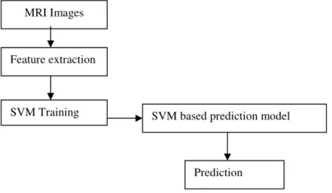
Machine learning provides methods, techniques and tools, which help to learn automatically and to make accurate predictions based on past observations [7]. Machine learning approaches to medical domains shows very promising research results. In this paper, the potential benefits of machine learning algorithm namely support vector machine are made use of for the automated prediction of epilepsy. Support Vector Machine (SVM) is a supervised learning algorithm for learning classification and regression rules from data. SVM is suitable for working accurately and efficiently with high dimensionality feature spaces. The proposed SVM based epilepsy prediction model is shown in Fig 1.
Fig. 1.Proposed SVM based epilepsy prediction model 2. Data acquisition
The MRI images of 350 epilepsy patients have been acquired on a 1.5 Tesla scanner of Siemens Magnetom Symphony, Erlangen, Germany, from Clarity Imaging Centre, Coimbatore. Axial, 2D, 5mm thick slice images, with a slice gap of 2mm have been acquired with 246*512 acquisition matrix and with the field view of range 220mm to 250mm. The image gray level in MRI mainly depends on three tissue parameters viz., proton density (PD), spin-lattice (T1) and spin-spin (T2) relaxation time. T1 and T2 are sensitive to the local environment; they are used to characterize different tissue types. T1, T2 and PD type images are mostly used by different researchers for different MR applications. Recently, the FLAIR sequence has replaced the PD image. FLAIR images are T2 weighted with the CSF signal suppressed. T1 shows higher intensity for white matter, T2 presents higher intensity for cerebrospinal fluid. Five sets of images namely Normal, Absence Epilepsy, Simple Partial Epilepsy, Complex Partial Epilepsy and General Epilepsy are taken into consideration.
3. Feature extraction
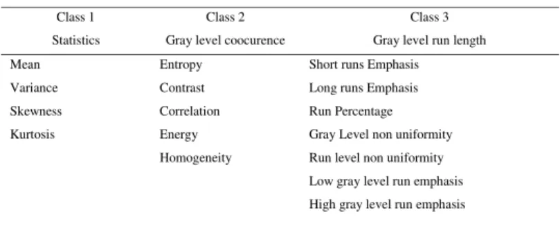
Three classes of textural features which characterize MRI images have been extracted and they are listed in Table 1. [8, 10].The features extracted from the MRI images of five categories are transformed into feature vectors and used for training. Each feature vector of size 16 is computed over the window size of ‘n×n’ pixel matrix.
The three categories of textural features are
• First order statistical features
• Second order statistics that are computed from spatial gray-level co-occurrence matrices (GLCMs)
• High order statistics that are computed from gray-level run length matrices (GLRLMs). MRI Images
Feature extraction
SVM Training SVM based prediction model
Table 1. Features Class 1
Statistics
Class 2 Gray level coocurence
Class 3 Gray level run length Mean Variance Skewness Kurtosis Entropy Contrast Correlation Energy Homogeneity
Short runs Emphasis Long runs Emphasis Run Percentage Gray Level non uniformity Run level non uniformity Low gray level run emphasis High gray level run emphasis
The first order statistical features such as mean, variance, skewness and kurtosis have been derived using (1)-(4).
Mean μ =
∑
− = 1 0)
(
G ii
iP
(1) Variance σ2 =∑
− =−
1 0 2)
(
)
(
G ii
P
i
μ
(2) Skewness m3 =∑
− =−
1 0 3)
(
)
(
G ii
P
i
μ
(3) Kurtosis m4 =∑
− =−
1 0 4)
(
)
(
G ii
P
i
μ
(4) where G is the number of gray levels in image and P (i) denotes the gray level intensity.The GLCMs are constructed by mapping the gray level co-occurrence probabilities based on spatial relations of pixels in different angular directions [8, 9]. The second order statistical features from gray level co-occurrence matrix (GLCM) such as entropy, contrast, correlation, energy and homogeneity are calculated as described in (5) - (9).
Entropy =
∑
j i j i P j i P , ) , ( log ) , ( (5) Contrast = 2 ( , ) , j i P j i j i∑
− (6) Correlation =∑
− − j i i j j i P j j i i , ) , ( ) )( (σ
σ
μ
μ
(7) Energy =∑
j i j i P , 2 ) , ( (8) Homogeneity =∑
−
+
j ii
j
j
i
P
,1
)
,
(
(9)where P(i, j)reflects the distribution of the probability of occurrence of a pair of gray levels (i, j), μi, μj, σi ,σj are the mean and
standard deviation values of GLCM.
The Gray Level Run Length Matrix (GLRLM) calculates characteristic textural measures from gray-level run lengths in different image directions [10]. The high order features from gray level run length matrices such as short run emphasis, long run emphasis, run percentage, gray level distribution, run length distribution, Low Gray-Level Run Emphasis and High Gray-Level Run Emphasis are calculated as described in (10) - (16).
Short Runs Emphasis are emphasized by dividing each element in P (i, j) by the square of its length (j). The denominator is the total number of gaps in the image and is calculated using the formula
∑∑
= = = G i R j j j i P SRE 1 1 2 ) , (θ
(10)Long Runs Emphasis measures distribution of long runs and is highly dependent on the occurrence of long runs and it is computed as
(
,
)
1 1 2θ
j
i
P
j
LRE
G i R j∑∑
= ==
(11) Run Percentage is the ratio between the total numbers of observed runs to the number of pixels in the image and is given by1 (, ) 1 1 2
θ
j i P j N RP G i R j∑∑
= = = (12) Gray Level Non-uniformity measures the similarity of gray level values throughout the image and is calculated as
∑ ∑
= =⎟⎟⎠
⎞
⎜⎜⎝
⎛
=
G i R jj
i
P
GLN
1 2 1,
(
θ
(13) Run Level Non-uniformity measures the similarity of the length of runs throughout the image and it is computed using the formula∑ ∑
= =⎟
⎠
⎞
⎜
⎝
⎛
=
R j G ij
i
P
RLN
1 2 1,
(
θ
(14) Low Gray Level Run Emphasis (LGRE) and High Gray Level Run Emphasis (HGRE) is introduced to separate textures that have equal SRE or LRE, but non-equal distributions of gray levels in the runs and are given asLow Gray Level Run Emphasis
∑∑
= ==
G i R ji
j
i
P
LGRE
1 1 2)
,
(
θ
(15)High Gray Level Run Emphasis
(
,
)
1 1 2P
i
j
θ
i
HGRE
G i R j∑∑
= ==
(16) where P (i, j | θ) is the element in GLRLM that define the number of runs of gray level i, with length j, in a specific direction θ, G is number of gray levels in image, R is the longest run in image and N is the number of pixels in the image.4. Support vector machine
The machine is presented with a set of training examples, (xi, yi) where the xi is the real world data instances and the yi are the
labels indicating which class the instance belongs to. For the two class pattern recognition problem, yi = +1 or yi = -1. A training
example (xi, yi) is called positive if yi = +1 and negative otherwise. SVMs construct a hyper plane that separates two classes and
tries to achieve maximum separation between the classes. Separating the classes with a large margin minimizes a bound on the expected generalization error.
The simplest model of SVM called Maximal Margin classifier, constructs a linear separator (an optimal hyper plane) given by w T x - y= 0 between two classes of examples. The free parameters are a vector of weights w which is orthogonal to the hyper plane and a threshold value. These parameters are obtained by solving the following optimization problem using Lagrangian duality. Minimize = 2
2
1
w
subject toD
ii(
w
τx
i−
γ
)
≥
1
,
i
=
1
,...,
l
.
(17)where Dii corresponds to class labels +1 and -1. The instances with non-null weights are called support vectors. In the
presence of outliers and wrongly classified training examples it may be useful to allow some training errors in order to avoid over fitting. A vector of slack variables ξi that measure the amount of violation of the constraints is introduced and the optimization problem referred to as soft margin is given in the equation (18). In this formulation the contribution to the objective function of margin maximization and training errors can be balanced through the use of regularization parameter C.
When the number of class labels is more than two, the binary SVM can be extended to multi class SVM [11]. Multiclass support vector machine can be trained either using direct method or indirect method. One of the indirect methods for multiclass SVM is one versus rest method. For each class a binary SVM classifier is constructed, discriminating the data points of that class against the rest. Thus in case of N classes, N binary SVM classifiers are built.
During testing, each classifier yields a decision value for the test data point and the classifier with the highest positive decision value assigns its label to the data point. The comparison between the decision values produced by different SVMs is still valid because the training parameters and the dataset remain the same.
One of the direct multiclass SVM is Crammer and Singer method and the formulation is given by
∑
∑
= = + n t i k N k kw C w 1 1 2 1ξ
τ subject tow
k( )
x
iw
k( )
x
ie
ik ik
k
i iφ
−
φ
≥
−
ξ
,
∀
≠
τ τ (18)where ki is the class to which the training data belong,
1
t,
k t
k
c
e
=
−
(19) The decision function for a new input data xj is( )
,
max
arg
^ j k k jf
x
d
=
(20) wheref
k( )
x
j=
w
τkφ
( )
x
j−
γ
k 5. Experimental setupThe data analysis and epilepsy prediction is carried out using SVMlight2 tool for machine learning. Five categories of feature vectors are labeled as 1 for Normal, 2 for Absence Epilepsy, 3 for Simple Partial Epilepsy, 4 for Complex Partial Epilepsy and 5 for General Epilepsy, The training dataset used for epilepsy prediction modeling consists of about 350 images with 16 features, where each category consists of about 70 images.
2 SVMlight is an open source tool.
The dataset has been trained using SVM light with most commonly used kernels such as linear, polynomial and RBF with different parameter settings for d, gamma and C–regularization parameter. The parameters d and gamma are associated with polynomial kernel and RBF kernel respectively.
The 10 fold cross validation method is used for estimating the performance of the SVM based trained models. The performance of the models is evaluated based on prediction accuracy of the models and learning time i.e., the time taken to build the model.
6. Results and discussion
The cross validation results of the trained models based on support vector machine with linear kernel are shown in Table 2.
Table 2. SVM linear kernel
Linear SVM C=0.1 C=0.2 C=0.3 C=0.4
Accuracy(%) 84 86.36 84.5 85
Learning time(secs) 0.02 0.02 0.03 0.04
The results of the model based on SVM with polynomial kernel and with parameter d and regularization parameter C are shown in Table 3.
Table 3. SVM polynomial kernel
d
C=0.1 C=0.2 C=0.3 C=0.4 1 2 1 2 1 2 1 2
Accuracy(%) 87 88 90 93 90 90 91 92
Learning time(secs) 0.1 0.3 0.1 0.8 0.9 0.2 0.2 0.3
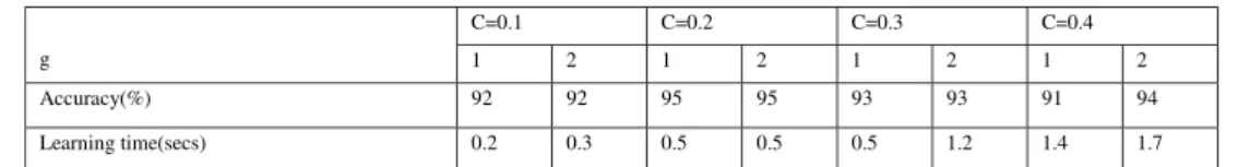
The predictive accuracy of the non-linear support vector machine with the parameter gamma (g) of RBF kernel and the regularization parameter C is shown in Table 4.
Table 4. SVM RBF kernel
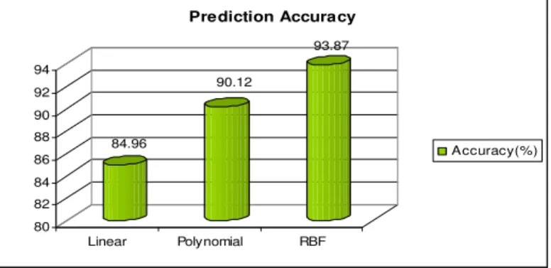
The average and comparative performance of the SVM based prediction model in terms of predictive accuracy and learning time is given in Table 5 and shown in Fig 2 and Fig 3.
Table 5. Overall performance of three models
Kernel type Accuracy(%) Learning time(secs) Linear 84.96 0.027 Polynomial 90.12 0.362 RBF 93.87 0.787 g C=0.1 C=0.2 C=0.3 C=0.4 1 2 1 2 1 2 1 2 Accuracy(%) 92 92 95 95 93 93 91 94 Learning time(secs) 0.2 0.3 0.5 0.5 0.5 1.2 1.4 1.7
84.96 90.12 93.87 80 82 84 86 88 90 92 94 Linear Polynomial RBF Prediction Accuracy Accuracy(%)
Fig. 2. Prediction Accuracy
0.027 0.362 0.787 0 0.1 0.2 0.3 0.4 0.5 0.6 0.7 0.8 Linear Polynomial RBF Learning Time Learning time(secs)
Fig. 3. Learning Time
As far as the epilepsy predictions task is concerned, accuracy plays major role in determining the performance of the MRI trained model than considering the learning time. From the above results, it is observed that the predictive accuracy shown by SVM with RBF kernel with parameters C=0.2 and g=2 is higher than the SVM with linear and polynomial kernel.
7. Conclusion
This paper demonstrates the applicability of supervised learning approach for solving epilepsy prediction problem. The epilepsy prediction task is modeled as classification problem and solved using a powerful supervised learning algorithm, support vector machine. The performance of SVM based epilepsy prediction models is evaluated using 10 fold cross validation and the results are analyzed. The results indicate that the support vector machine with RBF kernel gives the high prediction accuracy compared to other kernels. The outcome of the experiments indicate that Support vector machine models are capable of maintaining the stability of predictive accuracy, and can well be adopted for determining the type of epilepsy. Also, it was observed that the nonlinear techniques are more accurate in characterizing the epileptic features of MRI image and its associated category.
Acknowledgements
References
[1] H.P.Bruce. A Multidisciplinary Handbook of Epilepsy. Charles C. Thomas, Springfield, 1980.
[2] E. Haack, et al., Magnetic Resonance Imaging, Physical Principles and Sequence Design. Wieley-Liss, New York, 1999.
[3] Christian Loyek, Friedrich G. Woermann, Tim W. Nattkemper .Detection of Focal Cortical Dysplasia Lesions in MRI using Textural Features. pp. 432-436, 2008.
[4] M. C. Clark, L. O. Hall, D. B. Goldgof, L.P. Clarke, R. P. Velthuizen, and M. S.Silbiger. MRI Segmentation using Fuzzy Clustering Techniques. IEEE Engineering in Medicine and Biology, pp. 730-742, 1994.
[5] Forrest Sheng Bao , Jue-Ming Gao, Jing Hu , Donald Y. C. Lie , Yuanlin Zhang , and K. J. Oommen. Automated Epilepsy Diagnosis Using Interictal Scalp EEG. 31st Annual International Conference of the IEEE EMBS Minneapolis, Minnesota, USA, September 2-6, 2009.
[6] Maryann D’Alessandro, Rosana Esteller, George Vachtsevanos, Arthur Hinson, Javier Echauz, Brian Litt. Epileptic Seizure Prediction Using Hybrid Feature Selection over Multiple Intracranial EEG Electrode Contacts: A Report of Four Patients. IEEE Transactions on Biomedical Engineering, Vol. 50, No. 5, May 2003.
[7] T. Mitchell ”Machine learning” Ed. Mc Graw-Hill International edition.
[8] Haralick R, Shanmugam K, Dinstein I,etal. Textural features for image classification. IEEE Trans System Man Cybern. 1973; 3(6):610–21.
[9] R. A. Lerski, K. Straughan, L. R. Schad, D.Boyce, S. Bluml, and I. Zuna, MR Image Texture Analysis- An approach To Tissue Characterization, Magnetic Resonance Imaging, Vol. 11, pp. 873-887, 1993.
[10] Galloway M. Texture analysis using gray level runs lengths. Comp Graph Image Process. 1975; 4:172–9.
[11] K.Crammer and Y.Singer. On the algorithmic implementation of Multiclass SVMs, JMLR, 2001.
[12] Nello Cristianini and John Shawe-Taylor. An Introduction to Support Vector Machines and other kernel-based learning methods Cambridge University Press, 2000.
[13] Soman K.P, Loganathan R, Ajay V, Machine Learning with SVM and other Kernel Methods, PHI, India, 2009 .
[14] Joachims T, Schölkopf B, Burges C, Smola A, Making large-Scale SVM Learning Practical. Advances in Kernel Methods - Support Vector Learning, MIT Press, Cambridge, MA, USA,1999.