Reducing the Risk of Rail Transport of Hazardous Materials by Route Rationalization

Athaphon Kawprasert (Corresponding Author) Graduate Research Assistant Railroad Engineering Program

Department of Civil and Environmental Engineering University of Illinois at Urbana-Champaign B-118 Newmark Civil Engineering Laboratory, MC-250

205 North Mathews Avenue Urbana, Illinois 61801 USA Tel: (217) 244-6063 Fax: (217) 333-1924

Email: akawpra2@uiuc.edu

Christopher P.L. Barkan Associate Professor

Director - Railroad Engineering Program Department of Civil and Environmental Engineering

University of Illinois at Urbana-Champaign 1203 Newmark Civil Engineering Laboratory, MC-250

205 North Mathews Avenue Urbana, Illinois 61801 USA Tel: (217) 244-6338 Fax: (217) 333-1924

Email: cbarkan@uiuc.edu

Length of Manuscript: 5,268 words + 2 Tables + 6 Figures = 7,258 words Submission Date: December 7, 2007

Submitted for presentation at the 87th Annual Meeting of the Transportation Research Board and publication in Transportation Research Record

associated with each possible route, while simultaneously taking into account the production and consumption levels at each location in the network.

This paper presents a risk analysis model combined with an optimization technique to formally consider risk reduction by means of rationalization of the hazardous materials transportation rail route structure. The model is flexible and enables optimization of the route structure based on a variety of possible objective functions including minimization of mileage traveled, accident probability, likelihood of release, population exposure, and risk.

Keywords: Risk analysis, route rationalization, hazardous material, linear programming, optimization, objective function, Geographic Information System

INTRODUCTION

Railroads have placed a high priority on the safe transportation of hazardous materials for over a century (1). Traditionally, this activity focused on transportation packaging (2, 3, 4), product hazard identification, placarding, emergency information and response capability (5, 6). Railroads have developed special operating practices intended to reduce the likelihood or severity of accidents involving trains transporting certain hazardous materials (7). There has also been research on routing as an option to manage hazardous materials risk (8, 9, 10, 11). In recent years, the latter has gained increasing popular attention from municipalities eager to reduce the risk to their own constituents and analytical attention among researchers studying route planning for hazardous material transportation (12, 13). However, rerouting is neither simple nor necessarily effective at reducing risk because of physical constraints in the configuration of the rail network and the possible need to increase hazardous materials mileage traveled so as to avoid populated areas (10). Furthermore, the inevitable transferal of risk from one community to another raises significant political questions.

Due to security concerns and several fatal railroad hazardous materials accidents, railroads’ interest in all possible means of reducing hazardous materials transportation risk has intensified in recent years, especially for Toxic Inhalation Hazard (TIH) materials such as chlorine, ammonia and approximately two dozen other chemical products classified as TIHs (6). This has included increased attention to the traditional means of reducing risk mentioned above, as well as other options not previously given as much consideration. Among the latter category is rationalization of the transportation route structure for TIH’s shipped by rail. This approach differs from the type of routing discussed above because it does not simply involve trying to reroute traffic traveling between the current set of origins and destinations (OD pairs) to avoid

population centers en-route. Instead, route rationalization involves a comprehensive analysis of the entire route structure for a particular material and identifying opportunities to reduce the transportation volume or mileage traveled while taking into account the production and consumption levels at each location. This will often involve changing OD pairs to take advantage of shorter distances between particular production and consumption centers. In this paper, we introduce an optimization model to evaluate the route structure of a particular material to minimize several objective functions, including car-miles, probability of accident involvement and risk. The problem is similar to a traditional operations research topic known as the transportation problem (14) but is modified to account for the different objective functions.

We recognize that in practice there may often be constraints on the ability of rail carriers or chemical manufacturers to make the types of changes in distribution patterns considered in this paper. The model and results represent an idealized case that is intended to facilitate consideration of the approach. Our objective is not to suggest that such changes are easy or feasible in all cases. Instead, the purpose of this paper is to provide a structure and illustrative example to enhance evaluation of route rationalization as a possible risk management strategy.

The paper has several goals in support of this objective. One is to develop and present a basic, formal quantitative structure to enable consideration of route rationalization as an option for managing hazardous materials transport risk. The basic structure provides a framework to which additional constraints and factors can be added if more specificity or realism is desired. It can also help risk managers better understand the types of information needed and the factors to be considered if they wish to evaluate this option. Another is to use the model to consider a case study based on rail transport of an actual TIH. In addition to illustrating the model, it provides insight into the potential for risk reduction through use of this approach. And third is to preliminarily consider the effect of the use of different risk metrics as objective functions in the optimization process. This is of potential use to both researchers and practitioners because the different metrics may be more or less difficult to develop in different situations. Understanding the relationship of these metrics to one another may yield insight into the likely effect on risk in cases where more complete information is not available.

NATURE OF THE PROBLEM

Hazardous materials traffic originates and terminates at many different locations in the North American railroad network. Flows of a particular hazardous material, including TIHs, may involve fewer than a half dozen origin and destination points, or many hundreds of different points throughout the network. A simple example of a traffic-routing problem is illustrated in Figure 1a. Material produced at X and Y is shipped from X to Y, X to Z, and Y to X. Route rationalization involves reducing transportation volume by minimizing the car-mileage required to transport the material to the various destination points. This is manifested in two basic ways: either eliminating or reducing flows to locations that also produce and ship material, or by rerouting so that material is shipped to the nearest destination (Figure 1b). The computational complexity of the problem is related to the number of OD pairs, but the basic analytical methodology is the same.

FIGURE 1: Simple transportation network for a hazardous material A) without route rationalization, and B) with route rationalization

In the simple example illustrated in Figure 1b, material produced at X is consumed at X rather than being shipped to Y, and similarly, material produced at Y is consumed at Y. In addition, material produced at X and consumed at Z is instead supplied from Y because it is closer.

CASE STUDY

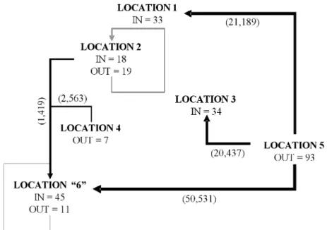
To illustrate route rationalization, we consider a set of traffic flows based on a particular hazardous material being transported on the North American railroad network. The network is comprised of six different locations (Figure 2) with the annual traffic volume (in carloads) at each location and the car-miles between each location (figures in parentheses). The route mileage between these locations was determined using rail routing software. We used the Princeton Transportation Network Model (PTNM) to develop maps of the traffic volume and directional flow but other suitable railroad network models could also be used for this purpose (15). After the route mileage is determined, the car-miles are calculated for each OD flow by multiplying the carloads by the mileage.

To rationalize this traffic flow pattern, we first assume that population exposure, accident probability, and other factors potentially affecting risk are homogenous across the entire route structure. Under these simplifying assumptions, risk will be proportional to the length of the route and the number of cars shipped. In this case, the problem reduces to the basic transportation problem in which the objective function is minimization of car-miles. This is synonymous with minimizing risk while holding shipment volume at each origin and destination constant. In reality, of course, these assumptions are too simplistic; there is considerable heterogeneity in various important factors affecting risk along the routes where hazardous materials are shipped. Furthermore, different decisions and policies may require differing consideration of various factors. Accordingly, the model must be capable of accounting for these if it is to provide useful results.

LINEAR PROGRAMMING MODEL FORMULATION

In this section, we formulate the linear programming (LP) model to determine the alternative traffic flow considered in the case study. As stated above, the objective function is initially set up to minimize total car-miles of hazardous material shipments with the constraint that incoming and outgoing traffic is held constant for each origin and destination. The constraint can be treated as demand and supply requirement at each location. The LP problem for minimizing the total car-miles is:

(1)

where: Vod = shipments (carloads) between origin o and destination d

Lod = mileage from origin o to destination d

Dd = total shipments (carloads) to destination d

So = total shipments (carloads) from origin o

The optimal network flow in which the total car-miles are minimized (Figure 3) can be found by solving the LP problem in Eq. (1). Using GAMS/Cplex, the optimal solution is 96,121 car-miles, which is 32.47 percent less than the original of 142,339 car-miles.

0 L , V and o , S V d , D V : o subject t L V miles -car Total Minimize od od d o od o d od od od od ≥ ∀ = ∀ = =

∑

∑

∑

FIGURE 3: Schematic diagram of the minimized car-miles network flow

RISK MODEL FORMULATION

The results presented in the previous section show the effect of reducing car-mileage on risk. However, as discussed previously, this does not guarantee risk reduction because the alternate, shorter routes might have a higher population density or accident rate. Therefore, a more sophisticated risk analysis needs to be conducted to determine other possible alternatives to minimize risk.

In this section, we discuss the formulation of a model for estimation of the risk associated with rail shipments of hazardous materials. The risk analysis is performed using a quantitative risk assessment (QRA) model to develop numerical estimates of the risk (16). Different levels of analysis can be performed depending on the degree of precision required for the problem under consideration. That is, accident rate and population density may be accounted for at the route level or track segment level. The model formulation presented here uses track segment-specific parameters in the risk analysis.

To begin with the risk model formulation, we assume that the occurrence of train accidents is a random event with a known rate of occurrence so that it can be modeled by using the Poisson distribution. Then, we can express the probability of k accident occurrences on a track segment of length L, P{N(L)=k}, as:

P{N(L)=k} = exp(–ZL)(ZL)k/k! (2)

where N(L) = the number of accidents on a track segment of length L k = 0, 1, 2…

Let A be the event that a tank car derailed in an accident and Ai that event occurring on track

segment i. We can express the probability that a tank car will be derailed in an accident on track segment i, P(Ai), as:

P(Ai) = 1–P{N(Li)=0}= 1–exp(–ZiLi)

≈ ZiLi (since ZiLi is very small) (3)

where Zi = the accident rate for track segment i

Li = the length of track segment i

For a route comprising n segments, we can also express the probability of a tank car derailment in an accident, P(A), by considering a non-homogeneous Poisson process:

∑ ≈∑ = ∫ = = = n 1 i n 1 i i i i i L 0 L Z ) L Z exp( -1 ) ZdL exp( -1 P(A) (4)

Accident rates, Zi, can be determined from previous accident statistics for individual track

segments or other segments determined to have similar characteristics. Here we use the FRA track class-specific accident rates developed by Anderson and Barkan (17). We also assume that

the probability of accident for hazardous material shipment does not depend on the type of material being transported (18).

Let R be the event of a hazardous material release from a tank car and Ri that event

occurring on track segment i. Then, we consider the probability of a hazardous material release

on track segment i, P(Ri). Assuming that there will be no release if there is no accident, i.e.

P(R|A′)P(Ai′) = ∅, so:

P(Ri) = P(R|A)P(Ai) (5)

where P(R|A) = the conditional probability of a hazardous material release from a tank car given that it is derailed in an accident

We estimate P(R|A) from the probabilities of lading loss developed by Treichel et al.

(19), which takes into account the design characteristics of the tank car. In this study, we

assumed that only one type of tank car is used to transport the material. If several types of cars are used but the effect of the different design characteristics is not of interest, the aggregated conditional probability, P(R|A)agg., can be computed using the weighted mean of the different car

types’ conditional probabilities:

P(R|A)agg. =

∑

∑

where wt = percentage distribution of tank cars with type t design characteristics

P(R|A)t = the conditional probability of a hazardous material release from a

tank car with type t design characteristics given that it is derailed in an

exposed to possible evacuation from the affected area due to a hazardous materials release. So, the consequence of a specific release scenario s for track segment i, Csi, is written as:

Csi = HsYi (8)

where Hs = affected area where people need to be evacuated or sheltered in place

for a specific scenario of release s

Yi = average population density in an exposure area corresponding to

track segment i

We determined the affected area, Hs, in accordance with the U.S. Department of

Transportation (DOT) Emergency Response Guidebook (ERG) recommended evacuation or shelter-in-place distances (6), corresponding to the particular chemical and release scenario. The

population density, Yi, is approximated by considering the weighted average number of people in

the census tracts coincident with the exposure area, which is defined herein as the area within the radius from the track center equal to the U.S. DOT ERG maximum evacuation distance for the worst-case release scenario for a particular hazardous material.

The ERG guidelines were developed and are periodically updated by the U.S. DOT. They are determined using a statistical model that incorporates sophisticated emission rate and dispersion models, historical release incident data, meteorological observations in North America and current toxicological exposure guidelines (6, 20). The ERG is widely used by the

emergency response community so it should be reasonably correlated with the events likely to occur in an actual hazardous materials spill. Furthermore, railroad costs in spill accidents are driven to some degree by the extent of the evacuation so use of the ERG-affected area as a metric for consequences provides some insight regarding relative railroad expenses. The ERG guidelines do not reflect injuries or fatalities due to a release. Instead they enable a relative comparison in terms of the number of people who might be affected by a release. The ERG guidelines are considered conservative and therefore may lead to overestimation of the number of people who will actually be affected. This is more likely to affect absolute estimates of risk than the relative estimates that are important in the analyses considered in this paper so we believe it is a satisfactory metric in the context of this study.

The final step is to define the risk metric. In our study, the annual expected number of people who potentially might need to be evacuated or sheltered in place according to the U.S. DOT ERG recommendations as a result of a hazardous material release, U, is considered as one possible metric. Another metric for route comparison is the average individual risk, V, defined as the total annual risk divided by total population of concern:

U =

∑

∑

∑

for the worst-case release scenario for a particular hazardous material To obtain the information on the distribution of risk outcomes, in addition to the expected risk, we developed a risk profile so that the change in probability of the incident with respect to the change in population exposure level can be observed and compared for each alternative. We prepared risk profiles (or “F-N” curves) by listing all pairs of P(Isi) and Csi, sorting by the latter

in a descending order, and plotting cumulative P(Isi) against Csi.

ESTIMATION OF THE RISK PARAMETERS

In this section, we discuss the estimation of the parameters affecting the risk for the case study in accordance with the formulation previously described. We determined the intermediate location points along the shipment routes using rail routing software. Then, using Geographic Information System (GIS) software, the route map layer was created for both the baseline and alternate route patterns using the U.S. DOT national railroad network data (21). The route created is divided

into segments, indicated by link ID in the network. For the purpose of illustrating the effect of differential accident rates, we estimated track quality and consequent derailment rate based on the type of traffic control system listed in the U.S. DOT GIS database because this is available for the entire U.S. rail network. However, if other data are available for a particular set of routes that enables more accurate estimation of accident rate, these could easily be substituted.

Track segment-specific accident rates are determined using accident rates for FRA track classes (17). The length of the track segments was determined from the GIS data. We assumed

all tank cars used were DOT-105 pressure cars with jacket and insulation, full head shields, and a tank thickness of 0.6875 in. These cars have a conditional probability of release given that they are derailed in a FRA-reportable mainline accident of 0.0691 (19).

Four different release scenarios were considered: small and large daytime spills, and small and large nighttime spills. We defined large spills as those in which more than five percent of the tank car’s contents are lost. The proportions of spill sizes from the distribution of quantity of lading loss for pressure cars in mainline accidents are 0.2213 and 0.7787 for small and large spills, respectively (19). In our analysis we assumed that shipments travel in daytime or

nighttime with equal likelihood; therefore, the proportions of daytime and nighttime release scenarios are 50 percent each for day or night or, 0.1106 for daytime/nighttime small spills, and 0.3894 for daytime/nighttime large spill. In this analysis we did not quantitatively consider the effect of time-of-day dependent population effects, but this can be factored into the model if the particular risk question warrants, and the data are available.

The hazard area of people affected for each release scenario is calculated using the U.S. DOT ERG table of initial isolation and protective action distances (6). For the material we chose,

the hazard areas for different atmospheric conditions and release sizes are: 0.011 mi2 for daytime/nighttime small spills, 0.092 mi2 for daytime large spills, and 0.252 mi2 for nighttime large spills. Finally, we used GIS to perform an overlay analysis of the hazard area and the population density to calculate the consequences of a release along each of the routes analyzed.

Subject to:

∑

∑

where: nod = shipments (carloads) between origin o and destination d

Nd = total shipments (carloads) to destination d

No = total shipments (carloads) from origin o

The objective function of the route rationalization model integrates three major elements in risk analysis: the probability of accident, the probability of release, and the consequence of release. This model can be modified depending on the particular purpose of the analysis. For example, if only release probability is of interest, the last two terms in the expression may be omitted. Furthermore, if risk control is required for any particular OD pair, the maximum risk level can be specified as a constraint in the model so that the risk for that particular route will not exceed the prescribed level. Thus, the route rationalization model should allow flexibility in the analysis to inform the desired policy and planning objectives.

RESULTS AND DISCUSSION

We used the route rationalization model in Eq. (11) to determine the set of optimal traffic flows for the case study, using minimization of three different objective functions: car-miles, release probability, and annual risk (Tables 1 and 2). The optimal flows for minimization of release probability and risk are shown in Figures 4a and 4b, respectively. For the particular hazardous material considered they are similar but differ in some details. Minimizing release probability reduced car-miles by 32.0 percent and risk by 16.3 percent whereas minimization of risk reduced car-miles by 32.5 percent and risk by 17.8 percent (Table 2). In this study, we assumed a single car design, so the flow with accident probability minimized is the same as the flow in which release probability is minimized; however, if a mix of cars with different release probabilities were used on different routes, then these would not be equivalent.

TABLE 1: Comparison of the effect of different objective functions on different annual risk metrics considered

Objective Function Minimized

Metrics Baseline

Traffic Flow Car-miles

Release

Probability Annual Risk Total Car-miles

Accident Probability Release Probability Total Risk

Average Individual Risk

142,339 0.01765 0.00122 0.12877 1.69x10-7 96,121 0.01289 0.00089 0.10581 1.38x10-7 96,722 0.01280 0.00088 0.10814 1.60x10-7 96,140 0.01288 0.00089 0.10558 1.38x10-7

TABLE 2: Percentage change in various metrics relative to the baseline case when different objective functions are used

Objective Function Minimized

Metrics Baseline

Traffic Flow Car-miles

Release

Probability Annual Risk Total Car-miles

Accident Probability Release Probability Total Risk

Average Individual Risk

142,339 0.01765 0.00122 0.12877 1.69x10-7 -32.5% -26.7% -27.0% -17.8% -18.3% -32.0% -27.3% -27.5% -16.3% -5.3% -32.5% -26.7% -27.1% -17.8% -18.3%

A

B

FIGURE 4: Schematic diagram of traffic flow when A) release probability is minimized and B) risk is minimized

In addition to the point estimates of average risk, an understanding of the distribution of risk outcomes is often useful for risk management decisions. This is particularly true regarding routing questions because routing is one of the few risk reduction strategies with the potential to affect the consequences of a release as well as the probability.

Use of risk profiles (Figure 5) allows comparison of the distribution of risk for the baseline traffic flow compared to the rationalized traffic flows based on the three different objective functions. As was the case with the average risk estimates, the risk profiles for the different objective functions do not differ much from one another, but are all lower than the baseline case. This difference is true across nearly the entire range of N, but the extent of the difference declines as N increases (Figure 6). This suggests that rationalizing the route structure for this particular hazardous material has a greater effect on reducing traffic in less populated areas of the route structure relative to the more highly populated portions. At the very highest values of N, there is no difference between the baseline and rationalized route structures, indicating that for this hazardous material exposure to the most densely populated segments is not eliminated by route rationalization. Nevertheless, there is an overall reduction in risk. Further study of other materials is needed to understand how typical these results of hazardous materials traffic in general.

FIGURE 5: Risk profiles for the baseline case compared to the rationalized route structures optimized using three different objective functions

FIGURE 6: Percentage reduction in the probability of N or more persons affected in the rationalized route structure in which risk is minimized compared to the baseline case

reducing the risk from rail transport of hazardous materials. The purpose is to introduce and illustrate the concept and explore the potential benefits that may be possible. We consider a simple case study based on the route structure of a TIH transported in railroad tank cars. The results indicate that for the product evaluated, route rationalization can reduce mileage, accident and release probability, risk and population exposure. In general, the extent of risk reduction possible will depend on the characteristics of the traffic pattern and other constraints of the particular optimization problem. For purposes of illustration and brevity, we relaxed some constraints in this study, including allowing traffic to travel via different railroads, neglecting the possibility of schedule conflicts or track unavailability, and not accounting for possible temporal variation in production capacity or demand. However the model was structured so that it can be adapted to incorporate these and other factors thereby enhancing its general applicability.

ACKNOWLEDGEMENTS

This research was supported by the University of Illinois Railroad Engineering Program. During a portion of this work the first author was supported by a grant from the Association of American Railroads. We are grateful to Diego Klabjan and Junho Song for their comments on the initial formulation of the model.

REFERENCES

1. Aldrich, M. Regulating Transportation of Hazardous Substances: Railroads and Reform, 1883-1930. Business History Review, Vol. 76, No. 2, 2002, pp. 267-297.

2. Barkan, C.P.L., T.S. Glickman, and A.E. Harvey. Benefit–Cost Evaluation of Using Different Specification Tank Cars to Reduce the Risk of Transporting Environmentally Sensitive Chemicals. In Transportation Research Record, No. 1313, TRB, National

Research Council, Washington, D.C., 1991, pp. 33–43.

3. Saat, M.R., and C.P.L. Barkan. Release Risk and Optimization of Railroad Tank Car Safety Design. In Transportation Research Record, No. 1916, TRB, National Research

Council, Washington, D.C., 2005, pp. 78–87.

4. Barkan, C.P.L., S. Ukkusuri and S.T. Waller. Optimizing Railroad Tank Cars for Safety: The Tradeoff Between Damage Resistance and Probability of Accident Involvement,

Computers & Operations Research, Vol. 34, 2007, pp. 1266–1286.

5. Moses, L.N. and D. Lindstrom. Transportation of Hazardous Materials: Issues in Law, Social Science, and Engineering, Kluwer Academic Publishers, Boston, 1993.

6. Pipeline and Hazardous Materials Safety Administration, U.S. Department of Transportation. Emergency Response Guidebook,

http://hazmat.dot.gov/pubs/erg/erg2004.pdf. Accessed June 29, 2007.

7. Association of American Railroads. Recommended Railroad Operating Practices for Transportation of Hazardous Materials, AAR Circular OT-55, Washington, D.C.,

January 4, 1990.

8. Glickman, T. Rerouting Railroad Shipments of Hazardous Materials to Avoid Populated Areas. Accident Analysis & Prevention, Vol. 15, No. 5, 1983, pp. 329-335.

9. Abkowitz, M., G. List, and A. E. Radwan. Critical Issues in Safe Transport of Hazardous Materials. Journal of Transportation Engineering, Vol. 115, No. 6, 1989, pp. 608-629.

10. Saat, M. R. and C. P. L. Barkan. The Effect of Rerouting and Tank Car Safety Design on the Risk of Rail Transport of Hazardous Materials. Proceedings of the 7th World Congress on Railway Research, Montreal, 2006.

11. Carotenutoa, P., S. Giordanib, and S. Ricciardellib. Finding Minimum and Equitable Risk Routes for Hazmat Shipments, Computers & Operations Research, Vol. 34, Issue 5,

2007, pp. 1304–1327.

12. Erkut, E., S. A. Tjandra, and V. Verter. Hazardous Materials Transportation, In

Handbooks in Operations Research and Management Science, Vol. 14, Barnhart, C. and

G. Laporte (Eds.). North-Holland, Amsterdam, 2007, pp. 539-621.

13. Glickman, T.S. et al. The Cost and Risk Impacts of Rerouting Railroad Shipments of Hazardous Materials, Accident Analysis and Prevention, 2007, doi:10.1016/j.aap.2007.01.006

14. Wagner, H. M. Principles of Operations Research. Prentice-Hall, Inc., Englewood Cliffs,

New Jersey, 1975.

15. Munshi, K., and S. C. Sullivan. A Freight Network Model for Mode and Route Choice,

Working Paper No.25, The University of California Transportation Center, University of California, Berkeley, California, 1989.

16. Center for Chemical Process Safety, American Institute of Chemical Engineers.

Guidelines for Chemical Transportation Risk Analysis, New York, New York, 1995.

17. Anderson, R. T., and C. P. L. Barkan. Railroad Accident Rates for Use in Transportation Risk Analysis. In Transportation Research Record, No. 1863, TRB, National Research

Council, Washington, D.C., 2004, pp. 88-98.

18. Anand, P. Cost-effectiveness of Reducing Environmental Risk from Railroad Tank Car Transportation of Hazardous Materials, Ph.D. Thesis, University of Illinois at

Urbana-Champaign, 2006.

19. Treichel, T. T., J. P. Hughes, C. P. L. Barkan, R. D. Sims, E. A. Phillips, and M. R. Saat.

Safety Performance of Tank Cars in Accidents: Probability of Lading Loss. Report

RA-05-02, RSI-AAR Railroad Tank Car Safety Research and Test Project, Association of American Railroads, Washington, D.C., 2006.

20. Brown, D.F. and W.E. Dunn. Application of a Quantitative Risk Assessment Method to Emergency Response Planning, Computers & Operations Research, Vol. 34, 2007,

1243–1265.

21. Bureau of Transportation Statistics, Research and Innovative Technology Administration, U.S. Department of Transportation. National Transportation Atlas Database,

www.bts.gov/publications/national_transportation_atlas_database/. Accessed May 1, 2007.