Visual Analysis for Extremely Large Scale Scientific Computing

(1)

V

isual Analysis for

E

xtremely

La

rge‐

S

cale

S

cientific

Co

mputing

D2.5 – Big data interfaces for data acquisition

Version 1.0

Deliverable Information

Grant Agreement no 619439

Web Site http://www.velassco.eu/

Related WP & Task: WP2, T2.4

Due date Mars 31, 2015

Dissemination Level

Nature

Author/s Benoit Lange, Toàn Nguyên

Contributors Alvaro Janda, Andreas Dietrich, Miguel Tinte, Jochen

Haenisch, Miguel Pasenau

(2)

Approvals

Name Institution Date OK

Author

Toàn Nguyên,

Andreas Dietrich,

Benoit Lange

INRIA 16/01/2015

Task Leader Benoit Lange INRIA

WP Leader Toàn Nguyên INRIA

Coordinator Change Log

Version Description of Change

Version 0.1 First draft version of the document

Version 1.0 First version of the document

Version 2.0 Update of the document with different contributions

Version 3.0 Added more contributions, comments, corrected styl,

numbering of sections, figures and foot‐notes

(3)

Table

of

content

1. Introduction _______________________________________________________ 5

2. Data Flow on the platform ____________________________________________ 8 2.1. Current state of the platform ____________________________________________ 9 2.2. Modules ____________________________________________________________ 11 2.2.1 Simulation ____________________________________________________________ 12 2.2.2 Ingestion ______________________________________________________________ 15 2.2.3 Storage _______________________________________________________________ 18 2.2.4 Access of Storage _______________________________________________________ 21 2.2.5 Analytics ______________________________________________________________ 22 2.2.6 Query Manager ________________________________________________________ 23 2.2.7 Visualization on the User Workstation ______________________________________ 25

3. Decomposition in Vqueries __________________________________________ 28 3.1. Session Queries ______________________________________________________ 28 3.2. Direct Result Queries __________________________________________________ 28 3.3. Result Analysis Queries ________________________________________________ 29 3.4. Data Ingestion Queries ________________________________________________ 29 4. Moving to HPC‐cloud _______________________________________________ 30 4.1. Simulation __________________________________________________________ 31 4.1.1 FEM simulations ________________________________________________________ 31 4.1.2 Discrete based simulations________________________________________________ 31 4.2. Ingestion ___________________________________________________________ 32 4.3. Storage _____________________________________________________________ 33 4.4. Access of Storage _____________________________________________________ 33 4.5. Analytics ____________________________________________________________ 34 4.6. Query Manager ______________________________________________________ 34 4.7. Visualization on the User Workstation ____________________________________ 34 5. Moving to Cloud ___________________________________________________ 35 5.1. Simulation __________________________________________________________ 36 5.2. Ingestion ___________________________________________________________ 36 5.3. Storage _____________________________________________________________ 36 5.4. Access of Storage _____________________________________________________ 37 5.5. Analytics ____________________________________________________________ 37 5.6. Query Manager ______________________________________________________ 37 5.7. Visualization on the User Workstation ____________________________________ 37 6. Conclusion _______________________________________________________ 38

(4)

7. References _______________________________________________________ 39

(5)

1. Introduction

By 2020, the amount of produced information will be huge. Tools used by scientific

community (simulation tool, or observation tools) will be able to produce more data than

ever before.

In fact as stated in [16] , science produces information using three paradigms: observational

Data, Experimental Data and Simulation Data.

In the case of observational data, data comes from unexpected events.

For the experimental use case, the production of information is performed in a fully

controlled environment, and all parameters are well known by scientists. This strategy

enables to reduce noise produced by external sources. This solution for the production of

information is mainly focused on closed environment like laboratories.

The final strategy used to produce data is based on simulations. A simulation is an execution

of a mathematical model, which is solved by a specific process. This resolution is performed

by iterative computation. This solution produces data without the need of doing a real

experimentation.

This discovery process has also evolved in the past few years. In fact, simulation software is

not anymore reserved by some specific communities (chemical, astrophysical, engineering,

etc.), but this kind of application is now used in all research fields. This evolution was guided

by the transformation of computing hardware. HPC environments will not be anymore the

architecture reference, the computation will be moved to cloud IT systems. This

transformation is lead by the evolution of the cost of such a kind of system. In a cloud

environment, CPU time is becoming cheaper than ever before. CPU time is becoming an

affordable resource.

This increase in computational data will lead scientists to move their mind to a novel

paradigm. The production of information is not anymore a problem; simulation tools exist

for a wide variety of domains. Today’s challenge is the management of the produced data. In

fact, IO operations have not been a main interest of the research community, and this kind

of operation suffers from this lack of attention by R&D. IO operations have not been

optimized compared to the evolution of the computation on CPU or GPU. To avoid issues of

writing latency, simulation engines do not write all data into the file system. Users of these

applications can select how many time steps shall be stored. Intermediary time steps

between different computations are considered not to be necessary.

In this project, we aim to provide a specific platform, which can deal with engineering data

by avoiding deleting intermediary information. This work targets to deal with two kinds of

datasets: already produced information (owned by scientific community) and computed

data produced by simulation engines. An exhaustive list of available resources for this

project is presented in Figure 1. This table shows all the requirements for external data. The

providers have limited access to the storage, and they are already using some strategy to

(6)

computed data. In the case of our partner, the targeted simulation tools (used by CIMNE and

UEDIN), can perform multiple time steps per execution. These multiple iterations may

produce very large amounts of data; thus it is necessary to use reduction methods in order

to deal with the produced dataset.

In this deliverable, we enlarge the notion of data acquisition from the “data ingestion”

concept (described previously in Deliverables D2.1 to 2.4) to the production of data. We

study in this document the workflow of all components: simulation, analytics tools, etc. It is

therefore not limited to the ingestion of data produced by a specific large‐scale application

by the VELaSSCo user panel.

It is deemed important to take into account the large volumes of data that are likely to be

stored, processed, produced and exchanged between the various modules of the platform.

This has a direct impact on the way the modules interact, on the required communications

protocols and on the latency, fault‐tolerance and, hence, the performance issues.

Further, e‐Science applications targeted by the VELaSSCo project are simulations using FEM

and DEM modeling approaches. However, many large‐scale collaborative projects have

integrated data stores to support collaboration among sometimes many international

stakeholders. This implies the management and effective access to and storage of large

volumes of remote heterogeneous data.

First, that data is ingested then analyzed and processed before dissemination and

visualization (Figure 2).

(7)

Next, the data might originate from various sources using different methods and tools,

including streaming to batch processing and transfers using messages and packet‐based

communication protocols.

Also, the data can range from very large numeric arrays to complex documents that include

text, videos and complex hyperlinks to each other. These data sets have some requirements

related to the storage method used. And depending on the storage method and complexity

the storage system has a more or less efficient data access system. An overview of the most

used methods is presented in Figure 3.

This means that effective and standardized communications and transfers approaches must

be used, on top of high‐speed and low‐latency hardware devices. Hierarchical memory

devices are common today, including hard disk drives, SSD, DRAM and caches to support fast Figure 3. NIST Big Data Interoperability Framework: Data Complexity [8]

(8)

data accesses to data and compute demanding applications. Also, data replication is a must

today in order to support fast and locally stored data, as well as fault‐tolerance.

In the rest of this document, we will discuss the flow of information of a HPC deployment of

the platform. Then we will study the impact on this communication flow in a HPC‐cloud

architecture. And finally, we will discuss the move to a pure cloud infrastructure. This study

will introduce our workflow decomposition based on Vqueries. If we compare our proposed

architecture with the architecture provided by NIST (see Figure 4), we can see that our

proposed architecture is compatible with the NIST proposal.

2. Data

Flow

on

the

platform

In this section, our interest is focused on the current state of the developed platform, and

then data flow of this platform. A simplified version of the architecture is presented in

Figure 5.

(9)

2.1.Current state of the platform

During the first year of the project, one solution has been elaborated upon by the

consortium to enable an early start the development of the VELaSSCo infrastructure. For this

solution, the hardware was provided by CIMNE; our compute platform is composed of two

dedicated nodes. The administration of these nodes has been given to VELaSSCo users in

order to be able to install all necessary software on the platform (without the HPC

restrictions) and for experimentation. These nodes are composed by two processors (Intel(R)

Xeon(R) CPU E5410 @ 2.33GHz), with 32Gb of memory. For the management of the

software stack, we have created a specific user named “velassco”, which was shared by

users of the platform. This user is used to store and start all necessary processes on the

platform.

Furthermore, as part of the deployment plan of the VELaSSCo platform, two dedicated

nodes for VELaSSCo platform have been already installed in the HPC cluster Eddie of the

University of Edinburgh. It is also expected to test the deployment of VELaSSCo platform on

this two nodes and later on the project to deploy the platform in Eddie HPC system involving

a large number of nodes. Currently, a refreshment of hardware and software stack is being

conducted in HPC Eddie systems by the cluster management team. Interestingly, the

refreshment actions of the Eddie are in line with the architecture designed for VELaSSCo

platform.

Our designed platform is decomposed into layers, and layers are split into components, see

Figure 5. Some of these components have already been described in previous deliverables, Figure 5. Schema of the VELaSSCo Architecture.

(10)

and their implementations already exist; thus the deployment of these specific parts can be

performed quickly. With the Hadoop ecosystem we are already covering a subset of

necessary tools, and some partners also provide some other tools for the platform.

For the simulation engine, CIMNE and UEDIN provide FEM and DEM simulation tools. These

tools already exist and are deployed on compute nodes outside of the VELaSSCo

architecture. This part of the project will not evolve; we will use a traditional strategy to

produce data.

The data layer is based of different components: Flume, HBase, Hive, a communication

component (Batch and RT), and HDFS (with HadoopAbstractFileSystem).

Flume is an existing tool, which can be used to aggregate information from multiple sources.

This tool is based on agents, they will gather information from one repository and store this

dataset into a targeted repository. These agents are in charge of merging data from multiple

sources. These agents are able to write data on different file systems or repositories. In the

case of this project we target to write information into HDFS (and from there further into

Jotne’s EDM after conversion into ISO 10303‐209) and HBase (a Big table system on top of

HDFS).

HBase is another piece of software used in this project. This tool offers a fast indexing

strategy for tabular data. This tool can be mapped on any file system, but was more suitable

for HDFS. This is used in the context of this project to offer a fast and efficient solution to

store and access data.

EDM (EXPRESS Data Manager) is an alternative storage of the VELaSSCo simulation data. It

does not follow the tabular paradigm, but the object‐oriented one that is specified in ISO

10303, STEP.

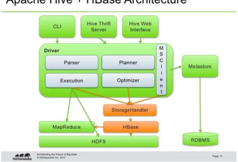
Hive is another tool used in the context of this project. This tool offers a simple query

language for a distributed file system. This method provides a query language based on SQL,

and offers, thus, the advantage of this simple language on top of HDFS. Hive enables to use

distributed computing with a well know query language. This tool is useful because it allows

interacting with a specific database stored on the file system, but it also enable to interact

with HBase. This solution offers a new strategy to interact with data stored in HDFS. Due to

its nature of supporting table‐based data, it is not applicable to the EDM‐use of the

VELaSSCo platform.

The storage layer of the platform is managed by the Hadoop infrastructure. Hadoop comes

with a dedicated File Storage system called HDFS. Using configuration files, it is possible to

use some other file system than HDFS Hadoop. An abstract layer on the Hadoop Java classes

brings this evolution of the platform. This strategy makes it possible to deploy different file

systems on a Hadoop ecosystem. We plan to use this feature to extend the Hadoop storage

system with the EDM DB.

The last component of the data layer is named “data query”. This component aims to

provide the necessary communication layout to interact with the storage layer. With this

component the engine layer of the platform will only use one communication protocol to

(11)

managing queries to the real‐time engine or the batch engine. This layer needs to be

developed.

The next layer of this platform is the engine layer. YARN, the resource scheduler and

manager of Hadoop is in charge of this layer. Four different modules compose this layer: a

query Manager Module, a monitoring module, a graphics module and an analytics module.

The monitoring module will use the existing zookeeper tool to monitor the platform. This

tool already exists and needs to be deployed for our own set of tools.

The analytics module is in charge of executing queries that process the stored data to extract

the information the scientist requests. For this purpose a specific computation is applied on

the existing data. An example of this feature is: extracting splines from a subset of the

model, extract a specific level of detail of the model, calculate the 0‐level iso‐surface of a

fluid simulation or the maximum damage result on a structural simulation. This component

can also write intermediary information to ensure a higher reactivity of the platform. This

extracted information is then passed to the graphics module.

The graphics module is in charge of prepare the Vquery results in a suitable way, so that the

information can be displayed by the visualization engines at high speed with minimal

latencies by using server side HPC compute and memory resources. To this end, the graphics

module converts the data into an internal representation. This module receives data from

the storage layer or from the analytics module, converts the extracted data set into a

specific format suitable for fast GPU rendering, and the resulting data structures are handed

over to the query manager module, which sends them back to the visualization client.

Moreover, the graphics module will handle streaming and progressive data transfer. Rather

than sending the complete data set of a query in one step, information is sent on demand in

small parts based on user input (e.g., depending on the position of a moving camera).

The final component of this platform is the query manager. This module is in charge of the

communication with the visualization client. This module offers a communication gateway to

the VELaSSCo platform. It is able to interact directly with the storage layer and to ask the

analytics module to do computation on some specific set of the stored data. This module is

also in charge of analyzing the complexity of a query to use the most suitable data flow

(direct access on the data or using the analytics module).

The last layer represents the visualization part of the platform. This layer is composed by a

single component and concerns the visualization part. This component is a plugin developed

by the consortium, which enables interaction between visualization software (iFX, GID) and

the VELaSSCo platform.

The next part of the document will provide a deeper description of each component and the

communication pipelines among them.

2.2.Modules

In this section we will discuss all the different workloads of the platform, with a special focus

(12)

2.2.1 Simulation

The data that is to be analyzed, processed and visualized using the VELaSSCo platform and

the visualization clients origins in numerical simulation programs that runs on HPC centers.

A simulation of a physical process is performed by solving the equations describing this

process using a discretization of the domain of the problem, depending on the method used

to solve these equations. Most numerical methods, like Finite Element Methods (FEM),

Finite Volumes (FV) are based on a discretization of the domain into small elements or cells

defining a mesh. These elements can be surface elements, such as triangles, or volume

elements, such as tetrahedrons. Other numerical methods like Discrete Element Methods

(DEM) use particles to represent the domain of the simulation. These particles can be circles,

spheres or can have more complex shapes. The output of these methods can be scalars,

vectors or tensors (that will be referred to as simulation results), which can be attached to

both nodes and elements. These simulation results can be viewed as attributes like typical

per‐face and per‐vertex attributes in computer graphics models: colours, normals, texture

coordinates, and so on. For example in the simulation of the aerodynamics of a racing car,

the domain to be represented is the air surrounding the car's body, and it can be

approximated using several millions of tetrahedrons.

The simulation program calculates the evolution of attributes like air pressure, velocity,

density or viscosity using this fixed volume mesh along all the time‐steps of the analysis.

Scientific simulations that run on High Performance Computing (HPC) clusters follow the

distributed memory paradigm and partition the huge domain meshes in small portions trying

to minimize the interface between these portions [17, 18] as shown in Figure 6. When the

simulation finishes, the post‐processing, i.e. result analysis and visualization, is usually

performed by merging these partitions, with their results, together in one single computer.

Figure 6. Simulation of the air flow around a telescope. The mesh with 24 million tetrahedrons was subdivided into 128 partitions in order to run on 128 cluster nodes as the colour map shows. Also the stream‐lines, lines tangent to the

(13)

2.2.1.1 FEMsimulations

Finite element simulation codes that run on HPC usually output their calculated results in

bursts, at each time‐step of the analysis. These results are stored, on a single file or on files

for each computation node that corresponds to one partition of the domain, on a

centralized, high efficient file system like Lustre, or NFS. In the case of the telescope

example, the central NFS file system contains all 128 files corresponding to the 128 sub‐

domains.

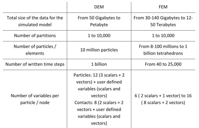
Table 1 shows for a single simulated model, the sizes of the data to be handled by the

system: size of the mesh, number of attributes per node or particle, number of expected

time‐steps, and number of sub‐domains for the single simulation.

DEM FEM Total size of the data for the simulated model From 50 Gigabytes to Petabyte From 30‐140 Gigabytes to 12‐ 50 Terabytes

Number of partitions 1 to 10,000 1 to 10,000 Number of particles /

elements 10 million particles

From 8‐100 millions to 1 billion tetrahedrons Number of written time steps 1 billion From 40 to 25,000

Number of variables per particle / node Particles: 12 (3 scalars + 2 vectors) + user defined variables (scalars and vectors) Contacts: 8 (2 scalars + 2 vectors + user defined variables (scalars and vectors) 6 ( 2 scalars + 1 vector) to 16 ( 8 scalars + 2 vectors)

Table 1 Characteristics of a single simulation to be handled by the VELaSSCo platform

A more detailed description of the simulation data was provided in the deliverable D1.3.

In the initial scenario of the project, the simulation data is already present and is to be

ingested in the platform from existing files.

To avoid the redundant storage of data both in files, from the simulation programs, and

inside the VELaSSCo platform, a more useful scenario contemplates that the results that are

being calculated by the calculation programs should be feed directly to the VELaSSCo

platform, by means of Flume agents.

To develop the last scenario, the project will also provide a Data Ingestion library that will

send the results to the platform at each time‐step of the simulation. The connection

(14)

Figure 7. Simulation program with the DataIngestion library to send results to the VELaSSCO platform.

Kratos Multi‐Physics is a free, open source framework for the development of multi‐

disciplinary solver and is being developed at CIMNE. This simulation program and was used

to generate the data provided by CIMNE by using the free GiDPost library. Kratos Multi‐

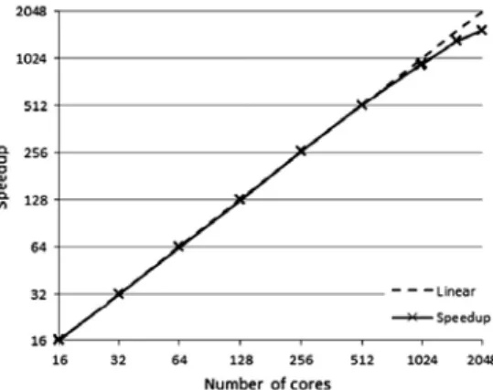
Physics has also been successfully ported to HPC environments as shown in Figure 8 [17].

Figure 8. Speedup achieved on the Telescope problem on the Marenostrum Supercomputer [19]

In this case, the VELaSSCo Data Ingestion library will be integrated in the GiD post library

that is already used by the simulation program to output the calculated results. This way the

interaction with the VELaSSCo platform will be transparent to the simulation code, requiring

only to set the destination of the results data (VELaSSCo_platform instead of

GiD_binary_files) and access credentials (user_name and password) in the unavoidably

initialization of the library.

This will constitute the test‐case for the previous mentioned scenario of ingesting simulation

data into the VELaSSCo platform from a running simulation program.

2.2.1.2 Discretebasedsimulations

In the case of discrete based simulations, the raw data is produced by a DEM simulation

solver. There already exist many different DEM simulation solvers that are extensively used

for both scientific and industrial applications. Some of them are commercial software such

as EDEM, PFC, StarCCM+ or DEMpack but there also available a wide range of open‐source

codes such as LAMMPS, LIGGGHTS, MercuryDPM or Yade. DEM computations are massively

parallelizable using space domain decomposition and data passing protocols such as MPI.

Therefore, most of the DEM simulation solvers are capable to work in distributed

environments such as traditional HPC systems.

In the case of DEM solvers, the calculation is computed based on discrete particles that

(15)

along the simulations is updated based on the forces acting on them by means of explicit

time integration of Newton laws. Thus, for each time‐step of the simulations, the solver

produces data related to the position, properties (mass, volume, …) and results (velocity,

angular velocity, …) of the particles and the contact forces network. A more detailed

description of the simulation data was provided in the deliverable D1.3.

The data writing process to files is conducted using a user predefined saving interval.

Typically, the simulation solver produces single files that contain the whole simulation data

for all time‐steps of the simulation or a data file per time‐step. Moreover, some of the DEM

solvers have the capability to save the data in a distributed way, i.e each node or processor

writes the data from the particles and contacts that it processes.

The data produced by the simulation solver needs to be ingested to VELaSSCo platform for

the post‐processing and analysis of the results. To this end, the simulation data is contained

in files that are read to ingest the data into the Big data table of VELaSSCo platform. For the

first prototype, it is considered that the simulations have already finished before the data

ingestion process is triggered. Nevertheless, for final version of the platform, it is expected

to explore the possibility to ingest the simulation data in a progressive way as the simulation

is running. In this latest case, a special triggering mechanism should be implemented in the

VELaSSCo. Platform.DataIngestion library (see Figure 7) in order to ingest the data into the

platform in an “on‐line” way.

2.2.2 Ingestion

This component is focused on the process of data ingestion. This module is in charge of the

communication between simulations nodes and the storage layer. This process performs a

formatting task for the dataset of the HPC nodes.

Figure 7 displays two main blocks that involved in the Ingestion process:

1. Simulation module in charge of generating simulation data files after each simulation

process completion. These files will be used as input for Ingestion and processing

module.

2. Ingestion & Processing part takes as input the simulation data files and processes

their information in order to store them into the database. To do so, this module

runs an ETL process1 where each simulation type is identified and processed in a

specific way.

Figure 9 shows that the simulation results being generated are ingested to the VELaSSCo

platform using the DataIngestion library and the Ingestion & processing module inserts this

data in the Storage module, which depending on the scenario store this data in HDFS or in

the EDM engine.

1

(16)

The implementation of the Ingestion module makes use of different tools and services to

achieve predefined functionalities. Basically, three functional blocks can be observed:

1. DataInjectorInstance component (described in VQueries chapter 3.4) will be

deployed as a RESTFul2 service. This first implementation allows asynchronous

communication between Simulation and Ingestion modules. This specific

communication pipeline comes from a web service, which uses callable through HTTP

Methods. Usually, a POST method will be used to send simulation data to processing

module. Example: URL: http://hpc_node:8080/DataInjectorInstance/rest/data/sendSimulData? Parameters: simulationName=DEM_box& analysisName=p3w& partId=003

2. The second tool used to store information in databases is Apache Flume3, which is in

charge of delivering large amounts of data through different agents. These

applications implement a simple and a flexible architecture based on streaming of a

data flow. Moreover, Flume provides an easy integration with some NoSQL

databases, like HBase4, which is the chosen one for our implementation.

In this context, it is important to describe how to integrate Apache Flume agents

regarding to the final data model. A flume agent has to be configured and deployed,

for this it is necessary to indicate the table and data model, which they are pointing

to. It can be configured through flume‐properties file:

2 http://en.wikipedia.org/wiki/Representational_state_transfer 3 http://flume.apache.org/index.html 4 http://hbase.apache.org/

Figure 9. VELaSSCo platform Ingestion sub‐workflow, from the simulation program, on the left, to the Ingestion & processing component and Storage module, in the Data Layer of the VELaSSCo platform.

(17)

The Flume agent configuration above specifies table name, column family, column

names and ROW_KEY information that HBase requires, in order to store the data

transported by the agent.

3. HBase is the NoSQL database chosen to represent simulation process information

and to provide access methods to retrieve such information efficiently. HBase is a

column‐oriented NoSQL database type which allows to insert information in different

column names within each column family (CF). Therefore, the number of CFs defined

in the Data Model is one of the important aspects in order to store and deliver this

information efficiently. Currently, three tables have been defined in order to satisfy

all data model requirements:

o VELaSCCo_Models: it stores general information regarding simulations already processed and stored, like size of the simulation and

validation/verification status.

# The configuration file needs to define the sources, the channels and the sinks.

# Sources, channels and sinks are defined per agent, in this case called 'agent'

agent.sources=avroSource agent.channels=channel1 agent.sinks=hbaseSink agent.sources.avroSource.type=avro agent.sources.avroSource.channels=channel1 agent.sources.avroSource.bind=0.0.0.0 agent.sources.avroSource.port=61616 agent.sources.avroSource.interceptors=i1 agent.sources.avroSource.interceptors.i1.type=timestamp agent.channels.channel1.type=memory agent.channels.channel1.capacity=100000 agent.channels.channel1.transactionCapactiy=10000 agent.channels.channel1.byteCapacityBufferPercentage=20 agent.channels.channel1.byteCapacity=800000 agent.sinks.hbaseSink.type=hbase agent.sinks.hbaseSink.channel=channel1 agent.sinks.hbaseSink.table=VELaSSCo_Models

# filling second column

agent.sinks.hbaseSink.columnFamily=TableInformation

agent.sinks.hbaseSink.batchSize = 5000

# splitting input parameters

agent.sinks.hbaseSink.serializer=org.apache.flume.sink.hbase.RegexHbaseEventSerializer agent.sinks.hbaseSink.serializer.regex=(.+)‐(.+)‐(.+)‐(.+)‐(.+)‐(.+)$ agent.sinks.hbaseSink.serializer.colNames=ROW_KEY,simulationID,boundingBox,validationSt atus,numberPart,otherData agent.sinks.hbaseSink.serializer.rowKeyIndex=0 agent.sinks.hbaseSink.serializer.ROW_KEY=ROW_KEY

(18)

o <simultation_ID>_metadata: It stores metadata information related to

simulations, like mesh type and result type information.

o <simulation_ID>_simulationData: It stores simulation data like coordinates, element connectivities, result values, etc. related to simulations.

Besides this, HBase will provide a data service access layer, which could eventually be

offered on an accessible manner. In this context, it can be easily integrated with

other tools to provide an accessibility layer. For instance, Apache Hive5 facilitates

integration6 as well as querying and managing large datasets residing in distributed

storage:

Figure 10. Apache HBase and Hive integration6

2.2.3 Storage

Different tools are included in this component, which already exist, see Figure 11. These

applications are parts of the Hadoop ecosystem; in addition to the scenario where the

simulation data is stored using HBase tables on HDFS, we will use also the JOTNE repository

EXPRESS Data Manager (EDM) for storage of engineering objects. Using Hadoop provides a

fully extensible storage framework for the VELaSSCo platform. As stated in D2.1, Hadoop

already supports multiple file systems to store data. It is also possible to use some

alternative storage solutions, such as the EDM DBMS. Developers and research communities

have developed several extension to Hadoop based on traditional database systems. In the

5

https://hive.apache.org/

6

(19)

case of this project, we will use this extensibility to provide the most suitable storage

platform. We already have identified some plugins for indexing data and extending Hadoop

storage to support the EDM Database as a storage system.

Figure 11. Zoomed view on the data storage layer of the platform.

Hadoop provides all necessary tools to distribute data among several nodes. This operation

is available through HDFS, which is a part of the Hadoop ecosystem. HDFS is a virtual file

system developed for Hadoop. To not force the utilization of this virtual file system an

abstraction layer was developed and was named HadoopAbstratFileSystem. With this

methodology, it is possible to extend Hadoop storage using any kind of File system. Several

examples have already been developed: QFS7, or KFS8, etc. As stated in the reference

document of the NIST, presented in Figure 12, storage can be specialized into two

categories, based on a File System paradigm, or on an indexing methodology. In a file system

environment, it is possible to benefit from the organization: centralized compared to

distributed. And a file system also enables to have an organized structure for files. This

organization is controlled by a file storage strategy: delimited, with a fixed length parameter

and using binary storage. In an indexed paradigm, data can be retrieved efficiently using

different strategies: in the case of relational database, key‐value data, column data,

document oriented data and graph data. In VELaSSCo we will extend this indexed paradigm

to include object storage that is compliant with ISO 10303, STEP, using EDM.

With the extensibility of Hadoop, it has been possible to use multiple strategies to access

data. Several plug‐ins have been developed to extend the Hadoop File System; an example is

based on an indexing strategy linked to the HDFS. In order to increase the access speed,

multiple solutions can be used at the same time. In this project, we plan to use at least two

plugins for different data access strategies, which will offer different ways to increase data

access speed. This first one will be HBase, and another one can be Hive (these tools are

designed to access data in batch, a specific process will be necessary to extract content in

real time). To provide a faster access than these two tools (and that still fit with the real‐time

requirement), the accessing strategy can be extended by Phoenix.

7

https://www.quantcast.com/engineering/qfs

8

(20)

For the commercial version of the VELaSSCo platform, we will provide a plug‐ins for the

Jotne partner storage solution EDM database. Jotne has developed an object‐oriented

database specially designed to store engineering data. Hadoop will be extended by two EDM

plug‐ins.

As depicted in Figure 11 and in Figure 14, one EDM plugin will be developed to allow the

EDM DB to read files from the Hadoop File System and to write to it. The VELaSSCo test

models will be read, whereas the EDM indexed database files will be written to HDFS; the

latter will port the EDM DBMS to fit with the distributed storage infrastructure.

Figure 14 shows that the second plug‐in resides in the YARN module. It translated the Query

Manager queries into EDM compliant queries and returns results in a format that is readable

by the VELaSSCo YARN implementation.

Figure 13. EDM Plug‐in for the data injection and direct data access. Figure 12. NIST Big Data Interoperability Framework: Data Organization

(21)

These two EDM plug‐ins will be the gateway between Hadoop and EDM.

2.2.4 AccessofStorage

To avoid complex communication between the engine and data layers, an access component

will be developed. This component is in charge of receiving queries from the Engine layer

and mapping them to the correct access plugin (HBase, Hive, etc.). With this strategy, the

engine layer performs only one kind of query, and this query is directly mapped to the

correct access software. The management of Real‐time and batch queries is managed by

mapping to the correct module HBase, Phoenix, etc.

All the communications with this component are represented in Figure 15. This component Figure 15. External communication component for the storage layer.

(22)

will interact with sub modules using the thrift API provided by these applications. Only the

HDFS IO is performed using the cli, command line interface, API.

2.2.5 Analytics

The analytics module is in charge of analyzing and processing the stored data. This processes

aims to produce new information in order to answer a requirement from the Query Manger

(QM). To ensure a fast production of the desired data, the QM can ask to produce

information using two different methods. Thus analytics can be performed using multiple

solutions and these solutions can be triggered at the same time. The module will also

provide a cost estimation of the data analytic query to help the Query Manager evaluate in

which mode is the analytics to be evaluated. For time consuming queries the QM will trigger

two analytic queries at the same time: one over the simplified version of the model to

provide fast feedback to the user and another one over the full‐resolution model. In

collaboration with the graphics module the results of the queries will be returned to the

client using streaming, progressive and render efficient protocols and formats.

Figure 16. Analytics module and its relation with other VELaSSCo modules.

This component is in charge of some specific queries that have already been identified.

An example of this query is GetBoundaryOfAMesh(). This query consists of extracting the

boundary of a mesh from a simulation model data stored in VELaSSCo. Data.Layer. The

workflow of the query can be observed in Figure 17. In this specific example, the analytics

module is in charge of the operation CalculateBoundaryOfAMesh that is composed of

several components involving the data storage module and the analytics module (see Figure

18).

Following the MapReduce v2 (MR) in YARN , the computation pipeline of this query can be

described as follows:

(23)

2. In the map phase of the application: extract from the data storage the elements of the mesh and simulation that the user specified in the query (component GetElementsOfLocalMesh). 3. Still In the map phase of the application: From the elements data of the mesh extracted from the data storage, the analytics module computes the unique triangles/lines of the volume/surface mesh, i.e. the boundary of the mesh. 4. In the reduce phase of the application: All the partial unique triangles/lines computed in the previous step are joined together, and the repeated triangles/lines eliminated. 5. Now the while boundary mesh is formatted for drawing by Graphics module. Figure 17. Workflow of the VQuery

GetBOundaryOfAMesh().

Figure 18. Components of the CalculateBoundaryOfAMesh operation from the Analytics module.

The communication pipeline to compute this query includes communication between the

different modules of the platform: o Query Manager  Analytics: the query manager requests the computation of the query to the analytics module together with the input parameters of the query previously specified by the user. o Analytics ↔ Data storage: the analytics module receives from the data storage module the data of the elements of the mesh o Analytics  Query Manager: The analytics module sends the result of the computation to the query manager and it will send to graphics module from formatting. 2.2.6 QueryManager

The goal of this component is to manage the VELaSSCo platform by providing all the

necessary stuff to communicate with users (through visualization) and sub modules of the

platform. This component directly interacts with YARN (Hadoop scheduler). This module is

(24)

must understand the data flow of the platform and ensuring some feed‐back to the user

while time‐consuming queries are being executed. This component has a smart feature,

which enables to pre‐execute some queries in order to reduce the execution time of these

queries. For this module, we have targeted two kinds of queries: simple and complex ones.

This module is the manager module of VELaSSCo, all queries are redirected to this module. It

is in charge of providing all the necessary mechanisms to communicate with all components.

Its goal is to simplify the communication process between all modules, and also between

layers.

When a query sent by the visualization tool is received by the QM, this query is analyzed,

and decomposed into sub queries, operations. This decomposition depends on the topic of

the query and also on the desired response time. To ensure a faster solution to retrieve the

information, asynchronous queries can be triggered. This module studies the desired query

and executes desired computation on data. For example this module can extract information

from a coarse resolution of dataset in order to provide a faster result.

As stated earlier, this module decomposes queries. These produced queries can be twofold:

simple and complex. A simple query directly retrieves information from the storage layer,

while complex queries produce content from a computation.

This decomposition into multiple queries brings some complexity of the system; in fact it is

possible to express a query into different aggregation of queries. Thus, it will be necessary to

provide an evaluation utility to the QM to ensure the best decomposition of a query. But it

is necessary to know that even with this tool, performances can reach less performance than

planned.

The flow process of this module is depicted here:  A query is received from the client.  QM analyses this query and determines the most suitable decomposition of the query. In this case, multiple solutions are possible: o Gather directly data from the storage layer o Execute an analysis on stored data o Execute an Asynchronous query, which can be:  Gather directly data from the storage layer  Execute an analysis on stored data  When the result is available a message from a previous process is executed, o QM asks the graphics module to gather the necessary information. Figure 19. Query Manager of VELaSSCo

(25)

o Graphics module gathers data, and compresses datasets to the suitable GPU friendly format.

o Information is sent back to the QM

 QM receives this information and sends it to the visualization platform.

The communication process is presented in Figure 20. In this figure, two execution

workflows are presented, the workflow with black hexagones respresents the simulation

data flow (from compute nodes to the storage layer), while the workload composed by

purple circles represents the communicaiton pipeline between a user and the storage layer.

2.2.7 VisualizationontheUserWorkstation

A user accesses the VELaSSCo platform by operating a local visualization client (see Figure

22). The visualization client is separated from the database infrastructure, and

communicates remotely with the platform by sending queries and receiving results.

In order to exchange information with the platform, the visualization client makes use of the

VELaSSCo access library as a communication layer. The access library provides a specific

application programing interface (API) for managing queries and results. It can be linked to a

visualization engine, which handles user input and displays query results on a local

workstation. As part of the initial VELaSSCo implementation GiD (CIMNE) [14] and iFX

(Fraunhofer) [15] are employed as visualization engines. Both GiD and iFX feature a plugin‐

mechanism to enable extensions. To attach the access library to the visualization engines, a

plugin for each framework will be developed, where each plugin will be linked to the library.

Keeping platform access in a separated library allows for targeting other frameworks besides

GiD and iFX.

(26)

Figure 21. Graphics module in the

VELaSSCo platform

Figure 22. Visualization client with the Access library to communicate with the VELaSSCo platform

On the client side, a user interacts with the graphical user interface of one of the

visualization engines. User actions are translated by the plugin component into a query

message that is sent to the access library. To communicate with the engine layer, the library

will make use of Apache Thrift [13] which interchanges information between the access

library and the query manager module in the VELaSSCo engine layer (see above). Sending a

query will trigger either retrieving simulation results (to be visualized on the client), or the

computation of analysis algorithms over the simulation data (also to be rendered on the

client). It is also possible to retrieve partial simulation data to be post‐processed in the

visualization client. The resulting data is sent back the same way to the visualization engine,

which then displays or processes the data. The scheme in Figure 23 shows the steps that

follows a request initiated by the used with the visualization client. The request is mapped

and formatted to a Vquery, VELaSSCo query, which then is packed and send to the platform.

The platform then unpacks it and passes the Vquery to the QueryManager for its processing.

Figure 23. Workflow of an VQuery initiated by the user on the visualization client, blue box at the top, and received by the QueryManager module of the VELaSSCo platform, below.

(27)

Figure 24 shows the operations present in the platform access library that performs the

previous detailed steps.

Figure 24. Components involved in the operations conforming the PlatformAccess library, tied to the visualization client.

On the server side, the graphics module within the platform’s engine layer is responsible for

preparing query results. This is done in such a way that information can be displayed by the

visualization engines at high speed with minimal latencies. To this end, the graphics module

converts the data into an internal format. Data structures resulting from this conversion are

handed over to the query manager module, which sends them back to the visualization

client. This workflow is reflected in the scheme of Figure 25.

Figure 25. Workflow of the returning results of a processed VQuery, top white box, which are formatted, packed and sent to the platform access library, which in turns hands the data to the visualization client.

Figure 26 shows the components involved in the operations that handles the reception of

the results of the processed Vqueries on the client side.

(28)

3. Decomposition

in

Vqueries

In this project, the workload execution is expressed by queries named: VELaSSCo queries

(VQueries). A VQuery is a global functionality of the VELaSSCo platform. A Vquery can

express functionality at the user level and also at the ingestion level. A VQuery is an

aggregation of operations (which is an aggregate of components), which can evolve at

different levels. The queries will be implemented for the two storage solutions in VELaSSCO:

Hbase and EDM. All of the preliminary queries are part of one of four classes. These classes

are presented and discussed in the rest of this section.

3.1.Session Queries

The group of session queries provides the frame for access to the simulation contents data.

They manage user login with corresponding session handling, control access to models and

maintain model meta‐data, such as, thumbnails and validation information.

The specification of the queries has shown the need for the following modules in the

VELaSSCo architecture:

‐ user access management ‐ session handling

‐ model administration.

All of those modules will be distinct building blocks of the VELaSSCo platform independent of

the storage solutions. Functionalities will need to be mapped to the corresponding modules

and data in EDM and Hbase.

3.2.Direct Result Queries

This VQuery class defines queries, which directly interact with the storage layer. This class is

currently decomposed into 12 queries, with two main objectives: extract information or

delete information.

The extracting queries of this class are dedicated to gather the information stored into the

storage layer. The information was stored in a hierarchical decomposition:  The access point of a dataset is the model,

 A model can may contain a static mesh and one or more analyses,  An analysis contains one or several steps,

 A Time Step may contain Meshes in the case of dynamic meshes,  A mesh contains some elements.

The access of all sub‐parts of the data set can be performed using different queries, for

example, the extraction of a vertex can be performed by: it is ID, or it is coordinates.

For the deleting queries, different queries are implied to remove each part of the dataset.

(29)

3.3.Result Analysis Queries

The Result Analysis Queries (RAQ) include queries that conduct computation over the

simulation data in order to produce new results that help to understand original raw results

from the simulation solver. Currently, this VQ class is composed of 4 queries:  GetBoundingBox

 GetResultForPoints.  GetBoundaryOfAMesh.

 GetDiscrete2ContinuumOfAModel.

In all cases, the RAQ involve operations and/or components related to a Data Storage

module that extract the whole or part of simulation data models. The simulation data is

stored in the storage layer and the extraction of data is conducted depending on the input

arguments (model id, mesh id, time‐steps, …) of the RAQ specified by the user.

In some cases the new results produced by the RAQ need to be saved temporally or

permanently inside the platform. These new results will be stored in memory, in files or in

the HBase tables of the data storage layer depending of their size.

3.4.Data Ingestion Queries

Data Ingestion Queries (DIQ) is one of the VQuery families defined in this chapter. This

family focuses on the process of data insertion into persistence layer and it is composed by

one component and five operations described in workflow below:

As exposed on Figure 27, Data Ingestion Query family is composed by only one component

to satisfy all operations described. This component (DataInjectorInstance) is in charge of

managing all the logic associated to Data Ingestion process through five main operations:

 GetInjectorInstance: this operation is based on the process of creating an instance of

DataInjector component deployed in HPC platform.

 InjectSimulationData: once DataInjector component is instantiated, the process is

aimed to read and insert simulation data files into final databases.

 RunETLProcess: this operation runs Extract Transformation and Load process, where

each type of simulation data information is processed properly to be sent to

databases

 SendDataToPipeline: the process of sending data to datastores (HBase) is

implemented in this operation using Apache Flume as the software manager used to

synchronize events with simulation data and HBase database accesses.

 WriteDataIntoNOSQLStorage: Finally, this operation writes data received from Flume

agents into HBase tables.

The workflow depicted represents the main functionalities identified during VQueries

definition. During implementation phase, the component will be deployed into HPC

(30)

4. Moving

to

HPC

‐

cloud

As stated in D2.3, our plan is to provide a scalable software stack, which enables to move

from a HPC to a HPC‐cloud or a cloud architecture. Thus, our software stack need to suitable

to support a hardware architecture evolution.

This strategy is necessary due to the evolution of scientific computing cluster. A traditional

compute solution (based on HPC) used by scientific community is too expensive in term of

energy. Now, a computation on HPC cluster is only run if it is necessary, or mandatory

(because of energy cost). Another issue with HPC cluster is the deployment cost. This kind of

platform uses high‐end computation nodes, which are very expensive.

HPC systems are also under used: due to the number of scientists which are allowed to

access them, and also lack on programing skills necessary to use all features of these

systems. This underuse of these clusters comes from the size of scientific community. In

term of efficiency, nodes are also underuse because of the development complexity for

these new nodes (see XeonPhi). To reduce the complexity of the development and increase

the use of the institutional clusters, the architecture are evolving and moved to cloud

DataIngestion OP‐11.300. GetInjectorInstance CO‐11.01. DataInjectorInstance OP‐11.301. InjectSimulationData OP‐11.302. RunETLProcess OP‐11.303. SendDataToPipeline OP‐21.304. WriteDataIntoNOSQLStorage

(31)

systems. This new kind of ecosystem offer new models and new capabilities to the scientific

communities. With this strategy we hope to provide a new way to use efficiently IT

resources.

In the rest of this section, we will discuss on each component and evaluate the impact of

moving to a HPC‐cloud cluster.

4.1.Simulation

4.1.1 FEMsimulations

Kratos Multi‐Physics has been successfully ported to HPC environments [17]. In the article

“From Large Scale to Cloud Computing” [20] the authors analyze the similarities and

differences of porting the mould filing application of the Kratos Multi‐Physics framework

from traditional HPC clusters to cloud.

As mentioned earlier cloud computing is very interesting because of the scalability and

dynamic resources it provides. It also eliminates the big cost and effort of setting up an

initial HPC‐cluster, its later expansion and whose profitability is tied to a continuous

workload that uses all computational resources.

The same tools and paradigms used to take profit on large HPC infrastructure, like OpenMP,

MPI, etc., can also be used on HPC‐cloud. The HPC‐cloud environments are also more flexible

and configurable than traditional HPC clusters and provides more control over the software

stack and Operating System. On the other side, the user of the simulation codes have less

control over the hardware, which is fixed, less potent and is renovated by the cloud provides

at its own schedule. Another drawback is the communication speed and higher latencies

between the HPC‐cloud nodes and also with the local machine, when downloading the

results.

Being careful when choosing the HPC‐cloud configuration results in good HPC‐cloud

configuration, similar to small or medium HPC‐clusters [21, 22, 23].

In the article “From Large Scale to Cloud Computing” [20] the authors conclude that the

problems of porting a simulation code to HPC cloud are similar than porting the same code

to a traditional HPC cluster for large scale computing. Some tuning has to be done in order

to distribute optimally the work‐load to compensate the possible heterogeneous machines

and network configurations.

4.1.2 Discretebasedsimulations

Most of the previously mentioned DEM simulation solvers (see section Discrete based

simulations2.2.1.2) are compatible with an HPC cloud infrastructure. Therefore, moving to

HPC cloud the simulations does not represent any important problem. Concerning the

advantages of moving simulation to HPC Cloud systems, it can be mentioned the flexibility

on the amount of computational resources (for example number of nodes) so that they can

(32)

observed a lower performance of the simulations on HPC‐cloud respect to traditional HPC

systems when the same computational resources are used in both cases.

4.2.Ingestion

The Data Ingestion module will be firstly moved to HPC‐Cloud environment in order to take

advantage of some capacities offered by the cloud‐computing paradigm within an HPC

environment. This approach must be especially careful due to the special capacities that HPC

offers and should not be affected by virtualization process. In this context, there could be

several hybrid solutions in order to make use of benefits from both paradigms. For instance,

it is possible virtualizing Data Injection component whilst making use of HPC to host

distributed file system and databases. Below in Figure 28, it is displayed an example of this

mixed approach.

Figure 28 displays a tentative HPC‐Cloud architecture, which covers Data Ingestion

functionalities requirements. Despite this, there could be other implementations, more

sophisticated if needed, depending on the demands and customization of requirements for

each use case. Some implementations may use some a specific master node in the cluster Figure 28 HPC‐Cloud architecture example: virtual machines (VMs) are deployed on physical nodes. Data Ingestion logic