© 2019. Ashfaq Ali Shafin. This is a research/review paper, distributed under the terms of the Creative Commons Attribution-Noncommercial 3.0 Unported License http://creativecommons.org/licenses/by-nc/3.0/), permitting all non-commercial use, distribution, and reproduction in any medium, provided the original work is properly cited.
Neural & Artificial Intelligence
Volume 19 Issue 3 Version 1.0 Year 2019
Type: Double Blind Peer Reviewed International Research Journal
Publisher: Global Journals
Online ISSN:
0975-4172
& Print ISSN:
0975-4350
Machine Learning Approach to Forecast Average Weather
Temperature of Bangladesh
By Ashfaq Ali Shafin
Stamford University Bangladesh
Abstract-
Weather prediction is gaining popularity very rapidly in the current era of Artificial
Intelligence and Technologies. It is essential to predict the temperature of the weather for some
time. In this research paper, we tried to find out the pattern of the average temperature of
Bangladesh per year as well as the average temperature per season. We used different machine
learning algorithms to predict the future temperature of the Bangladesh region. In the experiment,
we used machine learning algorithms, such as Linear Regression, Polynomial Regression,
Isotonic Regression, and Support Vector Regressor. Isotonic Regression algorithm predicts the
training dataset most accurately, but Polynomial Regressor and Support Vector Regressor
predicts the future average temperature most accurately.
Keywords:
machine learning, linear regression, isotonic regression, support vector regressor,
polynomial regression, temperature prediction.
GJCST-D Classification:
I.2.m
MachineLearningApproachtoForecastAverageWeatherTemperatureofBangladesh
Global Journal of Computer Science and Technology Volume XIX Issue III Version I
39 Year 2 019
(
)
D
Machine Learning Approach to Forecast Average
Weather Temperature of Bangladesh
Ashfaq Ali Shafin
Abstract- Weather prediction is gaining popularity very rapidly
in the current era of Artificial Intelligence and Technologies. It is essential to predict the temperature of the weather for some time. In this research paper, we tried to find out the pattern of the average temperature of Bangladesh per year as well as the average temperature per season. We used different machine learning algorithms to predict the future temperature of the Bangladesh region. In the experiment, we used machine learning algorithms, such as Linear Regression, Polynomial Regression, Isotonic Regression, and Support Vector Regressor. Isotonic Regression algorithm predicts the training dataset most accurately, but Polynomial Regressor and Support Vector Regressor predicts the future average temperature most accurately.
Keywords: machine learning, linear regression, isotonic regression, support vector regressor, polynomial regression, temperature prediction.
I.
Introduction
rediction for the future using the correct algorithm is viral nowadays. This prediction is applicable for the weather prediction as well. We can use machine learning to know whether it will rain tomorrow or what will be the temperature tomorrow. Machine learning algorithms can correctly forecast weather features like humidity, temperature, outlook, and airflow speed and direction. This sector is immensely dependent on previous data and artificial intelligence. Predicting future weather also helps us to make decisions in agriculture, sports and many aspects of our lives.
We aimed to predict the average temperature of Bangladesh in this research paper. As a subtropical country, Bangladesh has very different weather from other countries due to periodic disparities of rainfall, sophisticated temperatures, and humidity. Mainly three distinct seasons are present in Bangladesh, and those are Summer, Rainy, and Winter [1]. The summer season consists from March to June, while Rainy season lasts June to October and the Winter is from October to March. Even though Bangladesh is known as the six-seasoned country, mainly three seasons can be observed in this current time.
The dataset used in this paper contains the average temperature from the year 1901 to 2018 on a once-a-month basis. We calculated the sum of the Author: Lecturer, Department of Computer Science and Engineering, Stamford University Bangladesh, Dhaka, Bangladesh.
e-mail: shafinashfaqali21@gmail.com
values of temperature of the twelve months and then divided by 12 to get the average temperature of that particular year. Then we used different machine learning algorithms to extrapolate our findings and the generalize the output result.
After the modeling, also known as training or fitting in machine learning, we have forecasted the average temperature for Bangladesh in upcoming days using the machine learning prediction. Future weather forecast can use the predicted result.
II.
Literature Review
Mizanur et al. used a model, produced for predicting mean temperature that adjusted with ground-based watched information in Bangladesh during the time of 1979-2006. For the comprehension of the model execution, they have utilized the Climate Research Unit (CRU) information. Better implementation of MRI-AGCM got through approval procedure expanded trust in using it later temperature projection for Bangladesh[2].
An assessment of air temperature and precipitation conduct is significant for momentary arranging and the forecast of future atmospheric conditions. Patterns in precipitation and temperature at yearly, regular and month to month time scales for the times of 1981-2008 have been dissected utilizing BMD information and MPI-ESM-LR (CMIP5) model information. Likewise, the outcomes thus structure a decent premise of future examinations on temperature changeability. Thinking about all seasons (winter, pre-storm, rainstorm and post-storm), most extreme temperature has expanded altogether in all seasons except winter which is immaterial over the entire investigation zone for BMD information however for MPI-ESM-LR (CMIP5) model information highest temperature is on increment in the area. Heat over the whole area expanded by 0.29˚celcius and 5.3˚celcisus every
century individually for BMD information and
MPI-ESM-LR (CMIP5) model information [3].
Holmstrom et al. recommended a method to determine the highest and lowest temperature of the subsequent seven days, given the data of the past couple days [7]. They employed a linear regression model and a variation of a functional linear regression model. Expert weather forecasting services for the prediction outperformed the two models. As a classification problem, Radhika et al. used support vector machines for climate forecast [8]. Krasnopolsky
P
For seasonal average temperature, the following table (1) is used to calculate the average temperature. We have added the average temperature for those months respectively and then divided it by 4 for the seasonal average temperature.
Table 1:Months in the Season
Season Months
Summer March, April, May, June, Rainy July, August, September, October Winter November, December, January,
February c) Data Visualization and Statistics
First, we plot the corresponding average temperature against the years from 1901 to 2018 from the dataset. We can observe from figure 1, the lowest average temperature was 24.2055 in the year of 1905, and the highest temperature was 26.5927 in the year of 2018.
Figure 1:Average Yearly Temperature of Bangladesh from the year 1901 to 2018
Figure (2), (3), and (4) represent the seasonal
average temperature of Bangladesh from 1901 to 2018 of summer, rainy, and winter seasons respectively. The lowest average temperature was 26.93° celsius for
summer, 26.10° celsius for the rainy season, and 19.05° Celsius for winter.
Figure 2:Summer Season Average Temperature of Bangladesh from the year 1901 to 2018
Figure 3: Rainy Season Average Temperature of Bangladesh from the year 1901 to 2018
Global Journal of Computer Science and Technology Volume XIX Issue III Version I
40 Year 2 019
(
)
D
and Rabinivitz offer a crossbreed model that employedneural networks to model weather forecasting [9]. A predictive model based on data mining was presented in [10] to establish fluctuating weather patterns
III.
Methodology
a) Dataset
We collected the dataset from the website www.kaggle.com/yakinrubaiat/bangladesh-weather-dataset. This dataset contains the monthly average value of Bangladesh temperature and rain from
1901 to 2015. Then we manually, added the data from the year 2016 to 2018 from the Bangladesh Meteorological Department which is the official weather forecasting department of Bangladesh government.
b) Pre-processing
For yearly average temperature, we have added all the monthly average temperature of a particular year and then divided it by 12 to get the annual average temperature. A mathematical equation presented for the average temperature of a year in equation (1).
𝑇𝑇ℎ𝑒𝑒 𝑎𝑎𝑎𝑎𝑒𝑒𝑎𝑎𝑎𝑎𝑎𝑎𝑒𝑒 𝑡𝑡𝑒𝑒𝑡𝑡𝑡𝑡𝑒𝑒𝑎𝑎𝑎𝑎𝑡𝑡𝑡𝑡𝑎𝑎𝑒𝑒 𝑜𝑜𝑜𝑜 𝑦𝑦𝑒𝑒𝑎𝑎𝑎𝑎 𝑥𝑥=
( � 𝑎𝑎𝑎𝑎𝑒𝑒𝑎𝑎𝑎𝑎𝑎𝑎𝑒𝑒 𝑡𝑡𝑒𝑒𝑡𝑡𝑡𝑡𝑒𝑒𝑎𝑎𝑎𝑎𝑡𝑡𝑡𝑡𝑎𝑎𝑒𝑒 𝑜𝑜𝑜𝑜 𝑡𝑡ℎ𝑒𝑒 𝑡𝑡𝑜𝑜𝑚𝑚𝑡𝑡ℎ 𝑖𝑖 𝑖𝑖𝑚𝑚 𝑦𝑦𝑒𝑒𝑎𝑎𝑎𝑎 𝑥𝑥)/12 𝐷𝐷𝑒𝑒𝐷𝐷𝑒𝑒𝑡𝑡𝐷𝐷𝑒𝑒𝑎𝑎
𝑖𝑖=𝐽𝐽𝑎𝑎𝑚𝑚𝑡𝑡𝑎𝑎𝑎𝑎𝑦𝑦
Figure 4: Winter Season Average Temperature of Bangladesh from the year 1901 to 2018
Table (2) describes the overview of the yearly and seasonal average temperature data statistics is. Standard Deviation of the annual average temperature is 0.42 while the standard deviation for the summer, rainy, and winter is 0.41, 0.29, and 0.56 respectively.
d) Estimator Selection
In this paper, we have used several machine
learning algorithms described in table (3) to train our
data and to predict future average temperature.
Estimator Parameter
Linear Regression Default Isotonic Regression Default
Polynomial Regression Degree = 2 and 3 Non-linear Support Vector
Regressor (SVR) Degree = 3
Table 2:Dataset Statistical Overview
Attributes Year Yearly Average Temperature (in Celsius) Summer Season Average Temperature (in Celsius) Rainy Season Average Temperature (in Celsius) Winter Season Average Temperature (in Celsius) Count 118 118 118 118 118 Mean 1959.5 25.13 27.96 26.72 20.33 SD* 34.2077 0.42 0.41 0.29 0.56 Minimum 1901 24.21 26.93 26.10 19.05 25% 1930.25 24.86 27.69 26.55 19.96 50% 1959.5 25.06 27.96 26.69 20.24 75% 1988.75 25.31 28.24 26.87 20.67 100% 2018 26.59 28.94 27.60 21.59
Polynomial regression is a structure of regression analysis in which the connection between the independent variable 𝑥𝑥 and the dependent variable 𝑦𝑦 displayed as n-th degree polynomial in x. Polynomial relapse fits a nonlinear relationship between the worth of x and the corresponding conditional mean of y. In this paper, we have used polynomial
regression of 2nd-degree, and 3rd-degree equations represented as follows: 𝑦𝑦=𝑤𝑤0+ 𝑤𝑤1𝑥𝑥+𝑤𝑤2𝑥𝑥2+𝑒𝑒 (4) 𝑦𝑦=𝑤𝑤0+ 𝑤𝑤1𝑥𝑥+𝑤𝑤2𝑥𝑥2+𝑤𝑤3𝑥𝑥3+𝑒𝑒 (5)
Global Journal of Computer Science and Technology Volume XIX Issue III Version I
41 Year 2 019
(
)
D
Machine Learning Approach to Forecast Average Weather Temperature of Bangladesh
Table 3:Estimators Used in the Experiment and Their Parameter
𝑦𝑦=𝑤𝑤0+ 𝑤𝑤1𝑥𝑥 +𝑒𝑒 (2)
Here, 𝑤𝑤0and 𝑤𝑤1are the weight vectors, and 𝑒𝑒 is
the error term.
Isotonic regression is the method of fitting a freestyle line to a succession of perceptions under the accompanying requirements: the provided freestyle line needs to be non-decreasing all over, and it needs to lie as near the opinion as would be prudent.
The isotonic regression optimization is expressed by:
𝑡𝑡𝑖𝑖𝑚𝑚𝑖𝑖𝑡𝑡𝑖𝑖𝑚𝑚𝑒𝑒 � 𝑤𝑤𝑖𝑖
𝑖𝑖 (𝑦𝑦𝑖𝑖 − 𝑦𝑦𝑡𝑡𝑎𝑎𝑒𝑒𝑦𝑦𝑖𝑖)
2 (3)
Here 𝑦𝑦𝑖𝑖 is actual output, 𝑦𝑦𝑡𝑡𝑎𝑎𝑒𝑒𝑦𝑦𝑖𝑖 is a prediction,
and𝑤𝑤𝑖𝑖are strictly positive weights (default to 1.0).
Linear regression is a direct technique of demonstrating the connection between a scalar reaction, also known as the dependent variable and one or more explanatory variables or independent factors. The instance of one logical variable is called univariate linear regression. For more than one explanatory variable, the procedure is called multiple linear regression [4]. This term is unmistakable from multivariate direct relapse, where numerous associated ward factors are anticipated, as opposed to a single scalar variable. [5]
For one variable feature 𝑥𝑥, year in our case and target value 𝑦𝑦, the average output temperature the linear regression equation is:
For Support Vector Regressor (SVR), the model delivered by help vector arrangement depends just on a subset of the preparation information because the cost capacity for structure the model does not think about preparing focuses that lie past the edge. Comparably, the model created by SVR depends just on a subset of the preparation information, because the cost capacity for structure the model overlooks any preparation information near the model forecast. The equation for non-linear SVR represented as:
𝑦𝑦= � 𝑤𝑤𝑖𝑖𝑥𝑥𝑖𝑖 +𝐷𝐷 𝑚𝑚
𝑖𝑖=0 (6)
Here, 𝑤𝑤 is the weight vector, 𝑥𝑥 is the input vector of years, 𝑦𝑦 is being outputted vector of average temperature and b is the bias term, and n is the degree
of the equation. In our case, we have used n=3 for the
experiment.
IV.
Result Analysis
Figure (5), (6), and (7) represents the yearly average temperature for the regressors mentioned above. Linear Regression and Isotonic Regression are fitted in figure (5), while graph (6) and (7) adapted for Polynomial Regression and Support Vector Regressor.
From figure (5), (6), and (7) we can observe that, a. Isotonic Regression works best for the yearly
average temperature training dataset.
b. Both Polynomial Regression of 3rddegree and SVR
of 3rd degree tries to fit the training data as
accurately as possible.
c. Linear Regression works most poorly among all the estimators.
Figure (8), (9), and (10) represent the yearly summer season average temperature for the estimators. We used graph 8 for Linear and Isotonic Regression. Figure (9) and figure (10) embody the Polynomial Regression and SVR for the yearly summer season average temperature.
Global Journal of Computer Science and Technology Volume XIX Issue III Version I
42 Year 2 019
(
)
D
Here, 𝑤𝑤0,𝑤𝑤1,𝑤𝑤2,𝑤𝑤3are weight vectors, 𝑥𝑥 is the
independent input variable of year, 𝑦𝑦 is the output variable average temperature, and e is the error term.
Figure 5: Result Analysis of Linear Regression and Isotonic Regression on Training Data of Yearly Average Temperature
of Bangladesh from the year 1901 to 2018
Figure 6: Result Analysis of Polynomial Regression of Degree 2ndand 3rdon Training Data of Yearly Average Temperature
of Bangladesh from the year 1901 to 2018
Figure 7: Result Analysis of Support Vector Regressor of Degree 3rdon Training Data of Yearly Average Temperature
From figure (8), (9), and (10) we can observe that, a. Isotonic Regression works best for summer season
yearly average temperature training dataset.
b. Both Polynomial Regression of 3rd degree and
Polynomial Regression of 2nd degree tries to fit the
training data as accurately as possible.
c. Linear Regression works most poorly among all the estimators.
Figure 11, 12 and 13 represent the yearly rainy
season average temperature for the estimators. We used graph 11 for Linear and Isotonic Regression.
Diagram 12 and 13 personify the Polynomial
Regression and SVR for the yearly summer season average temperature, respectively.
Global Journal of Computer Science and Technology Volume XIX Issue III Version I
43 Year 2 019
(
)
D
Machine Learning Approach to Forecast Average Weather Temperature of Bangladesh
Figure 8:Result Analysis of Linear Regression and Isotonic Regression on Training Data of Summer Season Average
Temperature of Bangladesh from the year 1901 to 2018
Figure 9:Result Analysis of Polynomial Regression of Degree 2ndand 3rdon Training Data of Summer Season Average
Temperature of Bangladesh from the year 1901 to 2018
Figure 10: Result Analysis of Support Vector Regressor of Degree 3rdon Training Data of Summer Season Average
Temperature of Bangladesh from the year 1901 to 2018
Figure 11:Result Analysis of Linear Regression and Isotonic Regression on Training Data of Rainy Season Average Temperature of Bangladesh from the year 1901 to 2018
Figure 12:Result Analysis of Polynomial Regression of Degree 2ndand 3rdon Training Data of Rainy Season Average Temperature of Bangladesh from the year 1901 to 2018
From figure (11), (12), (13) we can observe that,
a. For the rainy season dataset, Isotonic Regression fits the dataset accurately than other estimators.
b. Both Polynomial Regression of 3rd degree and
Polynomial Regression of 2nd degree fits quite
similarly with a minimal margin line
c. SVR of 3rd degree performs better than Polynomial
and Linear Regressor.
We used the figures (14), (15), and (16) to plot different estimators result for the winter season average temperature dataset. In diagram 14, we applied Linear and Isotonic Regression for the winter season. Figure Regression and SVR for the yearly summer season average temperature, respectively.
After observing figure (14), (15), and (16), we conclude that,
a. Aimed at the winter season dataset, Isotonic Regression fits the dataset accurately than other estimators.
b. Both Polynomial Regression of 3rd degree and
Polynomial Regression of 2nd degree fits quite
similarly with a minimal margin line
c. SVR of 3rd degree performs better than Polynomial
and Linear Regressor.
For result analysis, we have used four estimators to predict the estimator’s outcome. These are Mean Squared Error (MSE), Mean Absolute Error (MAE), Median Absolute Error (MedAE) and R2_Score.
Mean squared error (MSE) of an estimator measures the normal of the squares of the blunders-that is, the standard squared distinction between the assessed qualities and the genuine worth. MSE is a
Global Journal of Computer Science and Technology Volume XIX Issue III Version I
44 Year 2 019
(
)
D
Figure 13: Result Analysis of Support Vector Regressor of Degree 3rdon Training Data of Rainy Season Average Temperature of Bangladesh from the year 1901 to 2018
Figure 14:Result Analysis of Linear Regression and Isotonic Regression on Training Data of Winter Season Average Temperature of Bangladesh from the year 1901 to 2018
Figure 15:Result Analysis of Polynomial Regression of Degree 2ndand 3rdon Training Data of Winter Season Average Temperature of Bangladesh from the year 1901 to 2018
Figure 16: Result Analysis of Support Vector Regressor of Degree 3rdon Training Data of Winter Season Average Temperature of Bangladesh from the year 1901 to 2018
hazard work, relating to the conventional estimation of the squared mistake misfortune. The way that MSE is quite often carefully positive (and not zero) is a direct result of haphazardness or because the estimator does not represent data that could create a progressively precise estimate [6]. If a vector of n likelihoods created from a sample of n data points on all variables, and Y is the vector of experimental values of the variable being forecast, then the within-sample MSE of the predictor is computed as:
𝑀𝑀𝑀𝑀𝑀𝑀= 1𝑚𝑚� ( 𝑌𝑌𝑘𝑘− 𝑌𝑌�𝑘𝑘 )2 𝑚𝑚
𝑘𝑘=1 (7)
Mean Absolute Error (MAE) is a proportion of the contrast between two consistent factors. Accept X and Y are factors of combined perceptions that express a similar of n focuses, where the i number point have organized (𝑥𝑥𝑖𝑖,𝑦𝑦𝑖𝑖). Mean Absolute Error (MAE) is the normal vertical separation between each position and the character line. MAE is likewise the normal flat separation between each point and the personality line. If a vector of n likelihoods created from a sample of n data points on all variables, and Y is the vector of experimental values of the variable forecast, then the within-sample MSE of the marvel. Instances of Y versus X incorporate correlations of anticipated versus watched, ensuing time versus starting time, and one method of estimation versus an elective strategy of evaluation. Consider a dissipate plot predictor computed as:
= 𝑚𝑚1� | 𝑌𝑌𝑘𝑘− 𝑌𝑌�𝑘𝑘 |2 𝑚𝑚
𝑘𝑘=1 (8)
The Median Absolute Error (MedAE) is especially fascinating because it is secure to exceptions. The misfortune determined by taking the middle of every apparent distinction between the objective and the forecast. If 𝑌𝑌�𝑘𝑘 is the predicted value of
then the Median Absolute Error estimated over n samples defined as:
𝑀𝑀𝑎𝑎𝑦𝑦𝑀𝑀𝑀𝑀 = 𝑡𝑡𝑒𝑒𝑦𝑦𝑖𝑖𝑎𝑎𝑚𝑚 (| 𝑌𝑌1− 𝑌𝑌�1|, … … , | 𝑌𝑌𝑚𝑚− 𝑌𝑌���𝑚𝑚|) (9) R2_Score represents the extent of fluctuation that has been clarified by the autonomous factors in the model. It gives a sign of decency of fit and subsequently a proportion of how well inconspicuous examples are probably going to be anticipated by the model, though the extent of clarified change. R2_Score will be in the range of 0.0 to 1.0. A higher value of R2_Score means better performance of the estimator. If a vector of n likelihoods created from a sample of n data points on all variables, and Y is the vector of experimental values of the variable being forecast, then the R2_Score of the predictor is computed as:
𝑅𝑅2𝑀𝑀𝐷𝐷𝑜𝑜𝑎𝑎𝑒𝑒 = 1− ∑ (𝑌𝑌𝑘𝑘− 𝑌𝑌𝑘𝑘 �)2 𝑚𝑚 𝑘𝑘=1 ∑𝑚𝑚𝑘𝑘=1�𝑌𝑌𝑘𝑘− 𝑌𝑌��2 (10) 𝑤𝑤ℎ𝑒𝑒𝑎𝑎𝑒𝑒𝑌𝑌�= 1𝑚𝑚 � 𝑌𝑌𝑘𝑘 𝑚𝑚 𝑘𝑘=1
Table 4: Yearly Performance Metric on Training Dataset
Mean Squared Error Mean Absolute Error Median Absolute Error R2_score
Linear 0.093863 0.242148 0.205785 0.539885
Isotonic 0.050341 0.172628 0.139777 0.835687
Polynomial 2 0.083724 0.230284 0.19991 0.617148
Polynomial 3 0.061494 0.197245 0.159327 0.722697
SVR 0.061455 0.189903 0.140335 0.712918
Table 5: Summer Season Yearly Performance Metric on Training Dataset
Mean Squared Error Mean Absolute Error Median Absolute Error R2_score
Linear 0.155614 0.318922 0.297744 0.3500776
Isotonic 0.107546 0.228602 0.236929 0.695183
Polynomial 2 0.154835 0.29976 0.272486 0.555278
Polynomial 3 0.14919 0.27711 0.257635 0.657899
SVR 0.151835 0.27976 0.262486 0.645278
Table 6: Rainy Season Yearly Performance Metric on Training Dataset
Mean Squared Error Mean Absolute Error Median Absolute Error R2_score
Linear 0.077955 0.206872 0.146128 0.3800776
Isotonic 0.030075 0.134821 0.11163 0.715183
Polynomial 2 0.066564 0.174726 0.139304 0.535278
Polynomial 3 0.0557 0.153632 0.124492 0.687899
SVR 0.056564 0.151726 0.121304 0.695278
Global Journal of Computer Science and Technology Volume XIX Issue III Version I
45 Year 2 019
(
)
D
Machine Learning Approach to Forecast Average Weather Temperature of Bangladesh
the k-th sample and 𝑌𝑌𝑘𝑘is the corresponding actual value, 𝑀𝑀𝐴𝐴𝐸𝐸
Table 7: Winter Season Yearly Performance Metric on Training Dataset
Mean Squared Error Mean Absolute Error Median Absolute Error R2_score
Linear 0.206298 0.370612 0.305485 0.472405
Isotonic 0.114431 0.265708 0.266803 0.697074
Polynomial 2 0.155757 0.307127 0.31012 0.594085
Polynomial 3 0.140985 0.305768 0.277769 0.609855
SVR 0.145712 0.307321 0.31021 0.614085
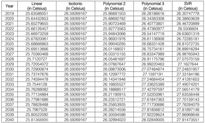
Table 8: Prediction of Yearly Average Temperature of Bangladesh
Year (in Celsius) Linear (in Celsius) Isotonic Polynomial 2 (in Celsius) Polynomial 3(in Celsius) (in Celsius) SVR 2019 25.63586051 26.59269167 25.86681503 26.28186616 26.30747778 2020 25.64432853 26.59269167 25.88692782 26.34383308 26.38603639 2021 25.65279655 26.59269167 25.90723469 26.40773801 26.46720899 2022 25.66126457 26.59269167 25.92773563 26.47360977 26.5506604 2023 25.66973259 26.59269167 25.94843066 26.54147719 26.63601319 2024 25.67820061 26.59269167 25.96931976 26.61136908 26.72285181 2025 25.68666863 26.59269167 25.99040295 26.68331428 26.81072735 2026 25.69513666 26.59269167 26.01168021 26.75734161 26.89916294 2027 25.70360468 26.59269167 26.03315155 26.83347989 26.98765943 2028 25.7120727 26.59269167 26.05481697 26.91175796 27.07570159 2029 25.72054072 26.59269167 26.07667647 26.99220463 27.1627644 2030 25.72900874 26.59269167 26.09873006 27.07484874 27.24831957 2031 25.73747676 26.59269167 26.12097772 27.1597191 27.33184196 2032 25.74594478 26.59269167 26.14341946 27.24684454 27.41281603 2033 25.7544128 26.59269167 26.16605527 27.33625389 27.49074201 2034 25.76288082 26.59269167 26.18888517 27.42797597 27.56514179 2035 25.77134884 26.59269167 26.21190915 27.52203961 27.63556448 2036 25.77981686 26.59269167 26.23512721 27.61847363 27.70159143 2037 25.78828488 26.59269167 26.25853935 27.71730686 27.76284079 2038 25.7967529 26.59269167 26.28214556 27.81856812 27.81897148 2039 25.80522092 26.59269167 26.30594586 27.92228624 27.86968648 2040 25.81368895 26.59269167 26.32994023 28.02849005 27.91473551
Global Journal of Computer Science and Technology Volume XIX Issue III Version I
46 Year 2 019
(
)
D
Table (4), (5), (6), and (7) represent the estimation of the estimators. We can observe that for training data, Isotonic Regression outperforms all the other estimators. As MSE, MAE, and MedAE are the lower and R2_Score of higher value means better performance for the estimator. We can notice that the boldfaced benefits of Isotonic Regressor perform better than other estimators. R2_Score for the yearly average temperature dataset is 0.835687, which is the highest value among all the datasets and estimators.
Polynomial Regressor of degree 3 and Support Vector Regressor of 3rddegree performs quite similar. All
the estimator’s values are the same as the other. Both
Regressors perform better than Linear Regression and second-degree Polynomial Regression.
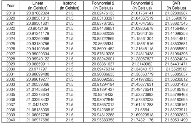
After training the dataset, we experimented with predicting the future yearly average temperature and seasonal average temperature. Table (8), (9), (10), and (11) denote the future average temperature for Bangladesh from 2019 to 2040. Extrapolated from the tables that, Isotonic Regression prediction is a constant value. As Isotonic Regressor cannot predict future projection for the average temperature, we should not rely on this estimator. The forecast for SVR or
Polynomial of degree 3, can be considered as the future
Table 9: Prediction of Summer Season Yearly Average Temperature of Bangladesh
Year (in Celsius) Linear (in Celsius) Isotonic Polynomial 2 (in Celsius) Polynomial 3(in Celsius) (in Celsius) SVR 2019 28.19047834 28.615 28.25449732 28.46365767 28.54480252 2020 28.19435532 28.615 28.26160216 28.49185427 28.58082584 2021 28.19823231 28.615 28.26876079 28.5209835 28.61857476 2022 28.20210929 28.615 28.27597322 28.55105987 28.65801114 2023 28.20598628 28.615 28.28323944 28.58209792 28.69906761 2024 28.20986327 28.615 28.29055947 28.61411216 28.74164722 2025 28.21374025 28.615 28.29793329 28.64711713 28.78562362 2026 28.21761724 28.615 28.30536091 28.68112735 28.83084182 2027 28.22149422 28.615 28.31284232 28.71615735 28.87711958 2028 28.22537121 28.615 28.32037754 28.75222166 28.92424923 2029 28.2292482 28.615 28.32796655 28.78933479 28.97200001 2030 28.23312518 28.615 28.33560936 28.82751127 29.02012093 2031 28.23700217 28.615 28.34330596 28.86676564 29.06834385 2032 28.24087915 28.615 28.35105637 28.90711242 29.11638708 2033 28.24475614 28.615 28.35886057 28.94856613 29.16395902 2034 28.24863313 28.615 28.36671857 28.9911413 29.21076218 2035 28.25251011 28.615 28.37463036 29.03485245 29.2564971 2036 28.2563871 28.615 28.38259596 29.07971412 29.30086648 2037 28.26026408 28.615 28.39061535 29.12574082 29.34357913 2038 28.26414107 28.615 28.39868854 29.17294709 29.38435384 2039 28.26801806 28.615 28.40681552 29.22134744 29.42292307 2040 28.27189504 28.615 28.41499631 29.27095641 29.45903642
Table 10: Prediction of Rainy Season Yearly Average Temperature of Bangladesh
Global Journal of Computer Science and Technology Volume XIX Issue III Version I
47 Year 2 019
(
)
D
Machine Learning Approach to Forecast Average Weather Temperature of Bangladesh
Year (in Celsius)Linear (in Celsius)Isotonic Polynomial 2(in Celsius) Polynomial 3(in Celsius) (in Celsius)SVR
2019 26.87127359 26.7 26.78574892 26.70392021 26.94289087 2020 26.87379679 26.7 26.78395995 26.69387951 27.00131911 2021 26.87631998 26.7 26.7820991 26.68342312 27.06501447 2022 26.87884318 26.7 26.78016639 26.67254536 27.13357378 2023 26.88136637 26.7 26.77816181 26.66124053 27.2065319 2024 26.88388956 26.7 26.77608535 26.64950297 27.28336802 2025 26.88641276 26.7 26.77393703 26.63732698 27.3635128 2026 26.88893595 26.7 26.77171684 26.62470689 27.44635609 2027 26.89145914 26.7 26.76942478 26.611637 27.53125518 2028 26.89398234 26.7 26.76706085 26.59811164 27.61754344 2029 26.89650553 26.7 26.76462505 26.58412513 27.70453908 2030 26.89902873 26.7 26.76211738 26.56967177 27.79155413 2031 26.90155192 26.7 26.75953784 26.55474589 27.87790315 2032 26.90407511 26.7 26.75688643 26.53934181 27.96291184 2033 26.90659831 26.7 26.75416316 26.52345384 28.04592527 2034 26.9091215 26.7 26.75136801 26.5070763 28.12631559 2035 26.9116447 26.7 26.74850099 26.4902035 28.20348922 2036 26.91416789 26.7 26.74556211 26.47282977 28.27689327 2037 26.91669108 26.7 26.74255135 26.45494942 28.34602125 2038 26.91921428 26.7 26.73946873 26.43655676 28.41041796 2039 26.92173747 26.7 26.73631423 26.41764611 28.46968347 2040 26.92426067 26.7 26.73308787 26.3982118 28.52347623
Year (in Celsius)Linear (in Celsius)Isotonic Polynomial 2(in Celsius) Polynomial 3(in Celsius) (in Celsius)SVR 2019 20.87662024 21.5 20.82475133 21.01764141 21.32800987 2020 20.88581813 21.5 20.83133397 21.04367519 21.3590079 2021 20.89501601 21.5 20.83787303 21.07047585 21.38827545 2022 20.9042139 21.5 20.84436851 21.09805678 21.41564907 2023 20.91341179 21.5 20.85082039 21.12643138 21.44098258 2024 20.92260968 21.5 20.85722869 21.15561304 21.46414814 2025 20.93180756 21.5 20.8635934 21.18561516 21.48503681 2026 20.94100545 21.5 20.86991452 21.21645115 21.50355891 2027 20.95020334 21.5 20.87619206 21.24813438 21.51964396 2028 20.95940122 21.5 20.88242601 21.28067827 21.53324034 2029 20.96859911 21.5 20.88861637 21.3140962 21.54431471 2030 20.977797 21.5 20.89476314 21.34840157 21.5528512 2031 20.98699488 21.5 20.90086633 21.38360779 21.55885037 2032 20.99619277 21.5 20.90692593 21.41972823 21.56232812 2033 21.00539066 21.5 20.91294194 21.45677631 21.56331439 2034 21.01458854 21.5 20.91891437 21.49476541 21.56185188 2035 21.02378643 21.5 20.9248432 21.53370893 21.55799468 2036 21.03298432 21.5 20.93072846 21.57362028 21.55180695 2037 21.0421822 21.5 20.93657012 21.61451283 21.54336161 2038 21.05138009 21.5 20.94236819 21.6564 21.53273911 2039 21.06057798 21.5 20.94812268 21.69929518 21.52002623 2040 21.06977586 21.5 20.95383358 21.74321176 21.50531499
Global Journal of Computer Science and Technology Volume XIX Issue III Version I
48 Year 2 019
(
)
D
Table 11:Prediction of Winter Season Yearly Average Temperature of Bangladesh
V.
Conclusion and Future Work
We can conclude our paper by extrapolating that, even though Isotonic Regression has performed better on the training dataset, for testing data, it performs very poorly. So, we cannot recommend this estimator for the prediction of upcoming annual or seasonal temperature for Bangladesh. We recommend using Polynomial Regression or SVR of higher degrees to predict the temperature for upcoming years.
Average temperature let alone will not be very useful for the weather forecast. That is why in the future, we want to forecast weather attributes like outlook prediction, rain prediction, and rainfall amount for the imminent future. Maximum temperature and minimum temperature prediction will also be sufficient for weather estimation.
R
eferences
R
éférences
R
eferencias
1. Weather Online. (2019). Bangladesh. Retrieved from
https://www.weatheronline.co.uk/reports/climate/Ban gladesh.html
2. Mizanur Rahman, M., Ferdousi, N., Sato, Y., Kusunoki, S., & Kitoh, A. (2012). Rainfall and temperature scenario for Bangladesh using 20 km mesh AGCM. International Journal of Climate Change Strategies and Management, 4(1), 66-80. DOI: 10.1108/17568691211200227
3. Bhuyan, M., Islam, M., & Bhuiyan, M. (2018). A Trend Analysis of Temperature and Rainfall to Predict Climate Change for Northwestern Region of
Bangladesh. American Journal of Climate Change,
07(02), 115-134. DOI: 10.4236/ajcc.2018.72009
4. David A. Freedman (2009). Statistical Models: Theory and Practice. Cambridge University Press. p. 26.
5. Rencher, Alvin C.; Christensen, William F. (2012), Chapter 10, Multivariate regression – Section 10.1, Introduction, Methods of Multivariate Analysis, Wiley Series in Probability and Statistics, 709 (3rd ed.), John Wiley & Sons, p. 19, ISBN 9781118391679.
6. Lehmann, E. L.; Casella, George (1998). Theory of
Point Estimation (2nd ed.). New York: Springer. ISBN 978-0-387-98502-2. MR 1639875
7. Holmstrom, M., Liu, D., & Vo, C. (2016). Machine Learning Applied to Weather Forecasting.
8. Radhika, Y., & Shashi, M. (2009). Atmospheric Temperature Prediction using Support Vector Machines. International Journal of Computer Theory and Engineering, 55-58. DOI: 10.7763/ijcte.
2009.v1.9
9. Krasnopolsky, V., & Fox-Rabinovitz, M. (2006). Complex hybrid models combining deterministic and machine learning components for numerical climate modeling and weather prediction. Neural Networks, 19(2), 122-134. DOI: 10.1016/j.neunet.
2006.01.002
10. Kumar, R., & Khatri, R. (2016). A Weather Forecasting Model using the Data Mining Technique. International Journal of Computer Applications, 139(14).