TR
OP
E
R
HC
RA
ES
E
R
PAI
D
I
LEARNING FROM IMAGES WITH CAPTIONS
USING THE MAXIMUM MARGIN SET
ALGORITHM
Jie Luo Francesco Orabona Barbara Caputo
Vittorio Ferrari
Idiap-RR-30-2011
AUGUST 2011
Centre du Parc, Rue Marconi 19, P.O. Box 592, CH - 1920 Martigny T +41 27 721 77 11 F +41 27 721 77 12 [email protected] www.idiap.ch
Learning from Images with Captions Using the
Maximum Margin Set Algorithm
Luo Jie, Francesco Orabona, Barbara Caputo and Vittorio Ferrari
Abstract—A large amount of images with accompanying text captions are available on the Internet. These are valuable for training visual classifiers without any explicit manual intervention. In this paper, we present a general framework to address this problem. Under this new framework, each training image is represented as a bag of regions, associated with a set of candidate labeling vectors. Each labeling vector encodes the possible labels for the regions of the image. The set of all possible labeling vectors can be generated automatically from the caption using natural language processing techniques. The use of labeling vectors provides a principled way to include diverse information from the captions, such as multiple types of words corresponding to different attributes of the same image region, labeling constraints derived from grammatical connections between words, uniqueness constraints, and spatial position indicators. Moreover, it can also be used to incorporate high-level domain knowledge useful for improving learning performance. We show that learning is possible under this weakly supervised setup. Exploiting this property of the problem, we propose a large margin discriminative formulation, and an efficient algorithm to solve the proposed learning problem. Experiments conducted on artificial datasets and two real-world images and captions datasets support our claims.
Index Terms—Weakly supervised learning, candidate labeling sets, images and captions, multi-class and multi-label classification, convex and non-convex optimization, large margin classifiers
F
1
I
NTRODUCTIONA huge amount of images with accompanying captions are available on the Internet. Websites selling various items such as houses and clothing provide photographs of their products along with concise descriptions. On-line newspapers (e.g. news.yahoo.com) have pictures illustrating events and comment them in the caption. These news websites are very popular because people are interested in other people, especially if they are famous (fig. 1). This motivates the recent interest in using captioned images for training visual classifiers. Exploiting the latent associations between images and text can lead to a virtually infinite source of training annotations, without any explicit manual intervention. The learned model can then be used in a variety of Computer Vision applications, including face recogni-tion, image search engines, and to annotate new images for which no caption is available.
There have been several works that study this problem on different applications and from different perspectives. Previous works have focused on associating names [4], • L. Jie is with the Idiap Research Institute, CH-1920 Martigny, Switzerland and the Swiss Federal Institute of Technology in Lausanne (EPFL), CH-1015 Lausanne, Switzerland. E-mail: [email protected]
• F. Orabona is with the DSI, Universit`a degli Studi di Milano, 20135 Milano, Italy. E-mail: [email protected]
• B. Caputo is with the Idiap Research Institute, CH-1920 Martigny, Switzerland. E-mail: [email protected]
• V. Ferrari is with the CALVIN research group, Computer Vision labora-tory, Swiss Federal Institute of Technology in Zurich (ETHZ), CH-8092 Zurich, Switzerland. E-mail: [email protected]
[26] and verbs [29] in the captions to the faces and body poses of people in news images, on learning character naming systems from TV series using scripts [16] and screenplays [10], on learning scene classification mod-els from tagged photos [3], [24], [41], and on learning object recognition models from an online nature ency-clopedia [40]. All these can be considered as weakly supervised learning problems, because each segment, face, pose, or object in the image is only indirectly, ambiguously labeled by the words in the captions.
The above tasks are more challenging than standard supervised learning tasks due to the correspondence am-biguity problem: it is not known beforehand which part of the image corresponds to which part of the caption. Moreover, not everything mentioned in a natural text caption appears in the image, and, vice-versa, not ev-erything in the image is mentioned by the caption. This is different from using tags which are guaranteed to describe the image, as in the Corel database [3]. On the other hand, natural language descriptions contain rich semantic information about the relations between different image regions and labels. For example, in fig. 1 (left), knowing what “waves” (verb) means would reveal who of the two imaged persons is “Barak Obama” (subject). The other way around, knowing who is “Barak Obama” would deliver a visual example for the “wav-ing” pose [29]. This connection between the name and the verb can be exploited to constrain the labeling: if a region is labeled by the name Barak, then it must also be labeled by “waving”. A labeling like “Barack-standing” is not valid given the caption. The caption sometimes enables to impose also other constraints. For instance, we know that Federer cannot appear twice in
an image, so no two image regions can take the same label “Federer”. As another example, captions some-times contain spatial position indicators. In the example of fig. 2, “Chervynsky” cannot be a valid label for the person in the middle. Such constraints can be used to prune the space of possible labelings, which facilitates learning [4], [26]. To the best of our knowledge, all existing algorithms are designed to explicitly incorporate a particular type of constraint. This means the algorithm has to be redesigned in order to integrate a new type of constraint.
In this paper, we propose a general, weakly supervised learning framework to model the problem of learning from images with captions. In this framework, each training image is represented as a bag of regions, and is associated with a set of candidate labeling vectors. Each candidate labeling vector encodes a possible labeling of all regions, with only one candidate labeling being fully correct. The set of candidate labeling vectors can be generated automatically from the captions using natural language processing (NLP) tools. This framework pro-vides a unified way to include many types of constraints. The contributions of this paper are: (i) we present a general framework which provides a principled way to include various types of constraints generated from the captions; (ii) we provide a theoretical analysis that justifies our framework, showing that under certain conditions it is possible to train classifiers even under this weakly supervised setup. Exploiting this property of the setup, we also propose a large margin discriminative formulation with an efficient stochastic gradient descent algorithm to optimize it; (iii) we present experiments on artificial datasets and two real-world datasets of images and captions. These experiments show that our approach achieves performance comparable to fully supervised approaches and outperforms other weakly supervised learning baselines; (iv) we release an open-source MAT-LAB implementation of our algorithm as part of the DOGMA library [34].
The rest of this paper is organized as follows. We re-view related works in sec. 2. Sec. 3 defines the problem of learning from images with captions and casts it into the candidate labeling sets framework. Sec. 4 presents the Maximum Margin Set (MMS) algorithm, which solves the learning problem defined before. We then report experiments on artificial datasets in sec. 5. We also apply our framework to two real-world tasks: learning face classifiers from news items (sec. 6) and learning both face and action (body pose) classifiers jointly (sec. 7). We show that learning both at the same time reduces the un-derlying corresponding ambiguity, and solves the name-to-face and verb-to-body assignment problems better than when tackling either task alone. We conclude the paper with discussions and possible extensions (sec. 8).
2
R
ELATEDW
ORKSImages and Captions/Tags: Learning visual classifiers from images with tags has been a very active line of
research in recent years [3], [24], [41]. These approaches must resolve the correspondence between image seg-ments and tags, which are typically nouns (e.g. tiger, grass, car). Because the tags are manually annotated to be descriptive for the image, algorithms can safely assume that nearly all tags should correspond to one or more image regions.
The problem of naming faces in images and videos using natural text sources has been particularly well studied [4], [10], [16], [26]. These works exploit the fact that often the names of the persons in the image are mentioned in the caption. Therefore, a caption contains possible labels for the faces in the corresponding image. However, an imaged person might not be mentioned in the caption and vice-versa. Hence, the level of noise and ambiguity in natural captions is typically higher compared to image tags. Various kinds of task-specific knowledge has also been integrated to improve learning performance, such as that two faces in one image can not be associated with the same name [4], or exploiting the motion of the mouth and the gender of a person [10]. Recently, a few works went beyond modeling a sin-gle type of word, and start to exploit the structure of sentences in the caption. Gupta and David [27] model prepositions in addition to nouns (e.g. ‘bear in water’, ‘car on street’). This prunes down the space of possible labelings. In Jie et al. [29], we model both names and action verbs jointly, and show that face and pose infor-mation help each other by reducing the correspondence ambiguity.
Related learning frameworks:Our problem is different from semi-supervised learning [46], where the learner has access to a set of labeled examples as well as a set of unlabeled examples. Instead, it is closer to the am-biguously labeled leaning or partially labeled learning setting [10], [23], [28], [31], where each training example is associated with multiple labels, only one of which is correct. Many approaches to such problems use the EM algorithm to estimate model parameters and the correct labels [23], [31]. The recent work of [10] is the most related to this paper, as it proposes a convex learning formulation based on minimizing an ambiguous loss function. In this paper, we generalize the ambiguous function to the multiple instances case, and use a non-convex learning formulation which achieves better per-formance than the convex learning formulation (sec. 4.5). Our work is also related to multi-label learning (MLL) [6], where each example is assigned multi-ple labels, any subset of which can be correct. Other related lines of research are multi-instance learning (MIL) [2], [14], and multi-instance multi-label learning (MIML) [44], [45]. MIML extends the two-label MIL setup to multiple labels. In both setups, instances are grouped into bags. The labels of the individual instances are not given. Instead, labels are given to the bags. However, contrary to our framework, in MIML noisy labels are not allowed: all the given labels for a bag are
B. Obama - Wave / M. Obama - Stand ? B. Obama - Wave B. Obama - Wave / M. Obama - Stand ? M. Obama - Stand R. Federer - Backhand / A. Roddick - Null ? R. Federer - Backhand
US Democratic presidential candidate Senator
Barack Obamawavesto supporters together
with his wifeMichelle Obamastandingbeside him at his North Carolina and Indiana primary election night rally in Raleigh.
Four sets ... Roger Federer pre-pares to hit a backhand in a quarter-final match with Andy Roddickat the US Open.
X
=
�
1
2
�
=
��
,
1
2
��
(Unknown)Y
=
{
[
y(1) :Federer,
y(2) :Backhand]
}
Z
=
�
Z
1Z
2�
=
�
[
z(1)1 :Federer,
z1(2):Backhand]
[
z(1)2 :Roddick,
z2(2):Null]
�
x x(1) x(2)Fig. 1. (Left, Middle) Two examples of image-caption pairs for the “who is doing what” task [29]. The face and upper body of the persons in the image are marked by bounding-boxes. We stress that a caption might contain names and/or verbs not visible in the image, and vice-versa. (Right) our candidate labeling set notation for the example in the middle. The imageX contains one regionx, which has two attributes: the person name and the verb describing the action he is performing. The candidate labeling setZcontains two candidate labeling vectorsz1andz2. Each labeling vector encodes one label for every attribute of the region. Importantly, note how [Roddick, Backhand] is not a candidate, as Roddick is not the subject of the verb “hit a backhand” in the caption. The true labeling vectorY is unknown and must be recovered by the algorithm.
Australia’s gold medalistGrant Hackett(C), Ukraine’s silver medalist Igor Chervynsky and USA’s bronze medalist Erik Vendtshow their medals following the 1500 metres freestyle race at the 10th World Swimming Championships in Barcelona July 27, 2003. Hackett clocked fourteen minutes 43.14 seconds.
Fig. 2. Example of an image-caption pair containing spatial indicators. The spatial indicator(C)indicatesHackettis the per-son in the middle, reducing the ambiguity in labels assignment.
correct. Moreover, current MIL and MIML algorithms usually rely on a ‘key’ instance in the bag [2] or they transform each bag into a single-instance representa-tion [45]. Instead, our algorithm makes an explicit effort to label every instance in a bag and to consider all of them during learning.
Latent Structure SVMs:Our algorithm is also related to Latent Structural SVMs [18], [42], where the correct labels are considered as latent variables. Wang and Mori [41] recently proposed a discriminative latent model for an-notating scene images given object nouns as tags (e.g. tiger, grass). They model the ground-truth region-to-annotation mapping and the overall scene label as latent variables.
3
P
ROBLEMD
EFINITIONIn this section, we define the problem of learning from images with captions, and establish the notation that will be used in the rest of the paper. We denote vectors by
bold letters, e.g.x,y, and use calligraphic letters for sets, e.g. X. Fig. 1 (right) gives an example of our setup. In sec. 6 and sec. 7 we will give several examples on how to cast existing problems into our framework.
Input data: The input is a collection of N image and caption pairs {Xi,Ci}Ni=1. An image Xi consists of Mi
regions Xi = {xi,m}mMi=1, and xi,m ∈ Rd. Each image
has an associated captionCi, which implicitly provides
partial labels for the image. Many real-world objects can belong to multiple concepts simultaneously. For example, an image region can bear several attributes: red (color), metal (texture) and car (object category). Quite often these attributes are correlated, so we argue that it is useful to model them together, using a label for each attribute. Without loss of generality, we assume that labelsYi ={yi,m}Mm=1i exist for every image region, but
they are unknown during training. We consider them as latent variables. The latent variables {yi,m}Mmi=1 encode
the labels for each region in the images. Each yi,m is
either a set of labels {yi,m(p)} P
p=1 or a single label yi,m
(i.e. P = 1), where P is the total number of attributes we model simultaneously. Each label yi,m(p) ∈ Y(
p) := {1,2,· · ·, K(p)
}indicates a specific attribute of a region, andK(p)denotes the number of possible different labels
for the attributep.
Candidate Labeling Sets: Our goal is to learn from the input image-caption pairs a classification function
f :x → y to classify regions of a new test image. The caption for the test image, when available, could still be used as an extra source of information to guide the prediction, but it is not required. Although the true labels of a training image are unknown, the accompanying caption usually describes the image. We assume that the labels of the regions only come from the caption. The learning algorithm should label withnullany region whose true label is not mentioned in the caption. A label corresponds to a word, or to a few words with the same meaning (e.g. “Barack Obama” and “President of the
USA”). In the rest of the paper we will only use the term “word”. Based on these assumptions, we generate the set of all possible assignments of the words in a caption to the regions in the corresponding image i, which we call Candidate Labeling Set (CLS) Zi. We use Li to denote the number of candidate assignments in Zi={Zi,l}lL=1i , with eachZi,l∈RP×Mi. In other words,
there areLi different possible combinations of labels for
the regions in the imagei. Only one of these candidate assignments is the true labeling, while the others are only partially correct or even completely wrong. Note that this isnotequivalent to simply associatingLi candidate
labels independently to each region. Instead, our defini-tion explicitly encodes the constrains between multiple regions and labels. To clarify this point, consider a simple example where we have two regions {xi,1,xi,2} with
two attributes each (color and object category). If it is known that they can only come from classes “red-car” or “blue-motor”, and that no two regions can have the same label, then zi,1 = [red-car,blue-motor],zi,2 = [blue-motor,red-car]will be the Candidate Labeling Vec-tors (CLVs) for this bag. Other possibilities such as
[blue-car,red-motor], [red-car,red-car]are excluded. An-other example could be an image with three regions, each of which could be labeled either “chair” or “ele-phant”. However, we know there cannot be both chairs and elephants in the same image. Such a structure can be encoded in our CLSs, but not in simple independent label sets for each region.
Constraints between words: As the size of the regions and the number of words grow, the number of admissi-ble labelings becomes intractaadmissi-ble. To keep the proadmissi-blem tractable, we could first filter out uninteresting words such as interjections and conjunctions, and maintain a dictionary with only the words we want to model. Each of these words will correspond to a different label. However, the number of admissible labelings can still be very large after the filtering. Let Wi be the number
of modeled words in the caption of an image i with
Mi regions. In the most general case, this image has Li = WiMi admissible labelings even when only one
label can be assigned to each region. In this uncon-strained scenario, the supervision information from the caption is very low for large Wi. Fortunately, captions
frequently contain valuable context cues which we can extract using NLP tools [1], [13]. These context cues can be translated into constraints to remove assignments from Zi. In addition, we can also reduce the size of Zi by incorporating high-level domain knowledge. As Li decreases when more constraints are added, the CLS Zi becomes less ambiguous. This scenario allows us to
design interesting learning algorithms, which we present in the next Section.
Our CLSs framework supports several types of useful constraints:
• [C1] Word type matches region type. For example, a
name can only be associated with a face region,
and/or a verb can only be associated with a person body region (where such regions are detected be-forehand, e.g. by an off-the-shelf face detector [38], [35] or an upper-body detector [21]). This type of constraint has been used in several works [4], [25], [29] (see fig. 1 for example).
• [C2] Sentence structure. Multiple words
grammati-cally connected in the caption must be assigned to spatially related image regions or even to the same region. Several kinds of connections in the caption can be used to eliminate labelings from Zi
which violate the resulting constraints: (a) noun-adjective [39], e.g. a “red car”, where both “red” and “car” are attributes of the same region; (b) name-verb [29], e.g. “Roger Federer hits a backhand”, “Roger Federer” is the subject of “hits backhand” and therefore point to the same person in the image. Therefore, any labeling that assigns “Roger Federer” to a certain face region, must assign “hits backhand” to the body region of the same person; (c) noun-preposition-noun [27], e.g. “sun in the sky” indicates that the two regions are close to each other, and the “sun” region is surrounded by the “sky” region. In general, this kind of connection conveys information about the spatial relationship between two regions.
• [C3]Uniqueness. Some words can only appear once
in the image. Two face regions in the same image cannot be associated to the same name [4], [25], [29].
• [C4] Spatial indicators. Captions sometimes contain
spatial position indicators [4] such as “(L)” and “left”. These suggest the relative spatial position of an image region w.r.t. the others. An example of this kind of connection is shown in fig. 2. The noun-preposition-noun structure discussed in [C2] can also be considered as a spatial indicator. Based on these constraints, we can explicitly enumer-ate the set of admissible assignmentsZifrom the caption Ci in several interesting problems. Hence, we replace
the captions by the CLSs {Zi}Ni=1. In a few other cases,
memory limitations prevents us from explicitly storing all assignmentsZi. In such a case we store the words and
the constraints, which we can use to generate subsets of
Zi “on the fly” during learning.
In this setting, the training data are provided in the form {Xi,Zi}Ni=1. Each image Xi is associated with a
set of CLVs Zi (including one which is fully correct).
Thus, our goal is to design a learning algorithm which learns classifiers from input data in this special form. Along the way to learning these classifiers, our algorithm also selects one CLV for each image, thus resolving the correspondence between image regions and words in the caption.
4
L
EARNING FROMC
ANDIDATEL
ABELINGS
ETS AND THEMMS A
LGORITHMIn sec. 3 we have discussed how to transform the prob-lem of learning from image-caption pairs into the CLS
problem. In this section, we first propose a large margin formulation of the CLS problem (sec. 4.1 to 4.4), then we present an efficient algorithm to optimize the proposed formulation (sec. 4.5 and 4.6).
Let X be the generic bag with M instances
{x1, . . . ,xm, . . . ,xM}, Z = {Z1, . . . ,Zl, . . . ,ZL} the
generic set of CLVs. Under this representation, X can be an image with M regions, and an instance xm is
a vector of appearance features describing the m-th region. An image region can either be a rectangular bounding box (e.g. a face [38]) found by an object detector, or an arbitrarily shaped segment found by an unsupervised segmentation algorithm [19]. Furthermore, let Y ={y1, . . . ,yM},Z={z1, . . . ,zM} be two labeling
vectors, where each element z,y ∈ YP is a label, with P denoted the number of attributes we model for each instance. We also assume a uniform prior over the CLVs in the CLSs, i.e. p(Zi) =p(Zj), ∀ Zi,Zj ∈ Z. Later, we
will discuss the possibility to extend these probabilities when the priors for each Zi are known.
4.1 Prediction functions
Given the training data {Xi,Zi}Ni=1, we want to learn a
linear prediction function which can work on individual instances. Motivated by the linear model in structural SVMs [32], we define the score functions as
sw(x, y(p)) =w·φ(x, y(p)),
where φ(·,·) is the feature mapping function, which creates a joint feature vector describing the relation-ship between the original input vector x and the la-bel y(p), with w being the classification hyperplane.
Intuitively, the score function quantifies how confident the model is to assign instance x to class y(p), and
the predicted label is the one with the highest score:
arg maxy(p)∈Y(p) sw(x, y(p)).
We also define the linear prediction function for an image region xas fw(x) =argmax y(p)∈Y(p) P X p=1 sw(x, y(p)) =argmax y∈Y w·ψ(x,y), where ψ(x,y) = PPp=1φ(x, y(
p)) is a joint feature
map-ping vector between the regionxand the labeling vector
y. This definition includes the special case of training different hyperplanes, one for each class. Indeedψ(x,y)
can be defined as ψ(x,y) = [ K(1) z }| { 0, · · ·, 0, φ(1)(x) | {z } y(1)-th , 0, · · · , 0, · · ·, K(p) z }| { 0, · · ·, 0, φ(p)(x) | {z } y(p)-th , 0, · · · , 0, · · ·], where φ(p)(
·) is a transformation that depends only on the data and the attributep. In this case the classifier w
is parameterized byPPp=1K(p) hyperplaneswy(p).
We can now define the score function for the image as Sw(X,Y), which intuitively is gathering from each
region inX the confidence on the labels encoded in Y. With the definitions above, we define the function Sas
Sw(X,Y) = M X m=1 sw(xm,ym) = M X m=1 w·ψ(xm,ym) =w·Φ(X,Y), (1)
where we haveΦ(X,Y) =PMm=1ψ(xm,ym). Given the
CLSZ, the predictions of the classifier are computed as
Fw(X,Z) = arg maxZ∈Z Sw(X,Z).
Remark 1: If the prior probabilities of the CLVs zl ∈ Z are also available, they can be incorporated into the score function by slightly modifying the feature mapping function in eq. (1) top(Zi)·Φ(X,Zi), where eachp(Zi)
is the prior probability forZi ∈ Z.
4.2 Ambiguous loss functions
In the supervised learning setup, many loss functions have been proposed based on minimization of a convex upper bound of an arbitrary risk measurement function
∆:Y×Y→R, which quantifies how much a predicted
label differs from the true label. A classic loss function is the 0/1 loss: ∆01(Z,Y) = M X m=1 P X p=1 1(zm(p)6=y( p) m ),
where 1(·) is the indicator function, Y = {y1, . . . ,yM}
are the true labels of regionsxm, andZare the predicted
labels. Hence, ∆01(Z,Y) simply counts the number of
mislabeled attributes over all regions.
However, in our setup the true labeling is unknown, and we only have access to the CLS Z, knowing that the true labeling vector is in it. So we propose to use an ambiguous version of the loss∆01, as a proxy for it:
∆A(Z,Z) = min
Z0∈Z∆01(Z,Z
0).
This loss function underestimates the true loss, while our goal is to minimize the true loss. Nevertheless, we can prove a strong connection between the ambiguous loss
∆A(Z,Z) and the true loss ∆01(Z,Y). The following
proposition shows that, in expectation, the ambiguous loss upper bounds the true 0/1 loss up to a constant multiplicative factor. To prove this, we use the theorems stated in [10, Proposition 3.1 to 3.3], and define an ambiguity degreefactorηfor a regionxm. The value of η
corresponds to the maximum probability of a noise label (i.e. ∀y ∈ Y(p)\ym(p)) co-occurring with a true labely(mp)
in the CLSZ, over all labels and examples generated by an unknown distribution.
Proposition 1: E[∆01(Z,Y)]≤ 1−η1 E[∆A(Z,Z)] Proof [Sketch]: Define
∆A(z(p) m ,Z (p) m ) = min z0∈Z(p) m ∆01(zm(p), z 0) =1(z(p) m ∈ Z/ (p) m )
the ambiguous loss for a single region xm and an
attribute p, with Zm(p) being the corresponding CLS for
the region. So we can use Proposition 3.1 of [10] to obtain
E[∆01(zm(p), y (p) m )]≤ 1 1−ηE[∆A(z (p) m ,Z (p) m )].
Using the definition of the true 0/1 loss and the linearity of expectation, and summing over mandp, we have
E[∆01(Z,Y)]≤ 1 1−ηE "XM m=1 P X p=1 1(z(p) m ∈ Z/ (p) m ) # ,
while using the relationship that Sm,pZ (p) m ⊇ Z, we obtain E "XM m=1 P X p=1 1(zm(p)∈ Z/ ( p) m ) # ≤E[∆A(Z,Z)] .
Combining them results in Proposition 1. Remark 2: The tightness of the above bound directly relates to the ambiguity degree η. When η = 0, we have only one labeling vector in every labeling set, i.e.
Li = 1. In this case, the problem becomes standard
supervised learning, and the bound is tight. On the other extreme, when η = 1, which means a certain noise label always co-occurs with a true label y(p), it
is impossible to distinguish them. One weakness of the stated bound is that it becomes very loose when there is a noise label that makes η very large, because thatη
equals the maximum probability of co-occurring among all the possible noise labels, although it only affects a few true labels. Nevertheless, using the extensions of Proposition 3.2 and Proposition 3.3 in [10], it is possible to obtain label-specific bounds, which enable to retain good learning performance on the subset of labels with low label-specific ambiguity degrees.
Hence, by minimizing the ambiguous loss we are actually minimizing an upper bound of the expected true loss. It is known that direct minimization of this loss is hard [12]. Therefore, in the following we intro-duce another loss that upper bounds ∆A which can be
minimized efficiently: `A(X,Z;w) =|max ¯ Z∈Z/ ∆A(Z,¯ Z) +Sw(X,Z¯) −max Z∈ZSw(X,Z)|+ , (2)
where |x|+ = max(0, x). The following proposition
shows that `A upper bounds∆A.
Proposition 2: `A(X,Z;w)≥∆A(X,Z;w) .
Proof :Define zˆ= arg maxz∈YM S(X,z;w). If Zˆ ∈ Z
then`A(X,Z;w)≥∆A(X,Z;w) = 0. We now consider
the case in whichZˆ∈ Z/ . We have that
∆A(X,Z;w) ≤∆A(Z,ˆ Z) +Sw(X,Zˆ)−max z∈ZSw(X,Z) ≤max¯ Z∈Z/ ∆A(Z,¯ Z) +Sw(X,Z¯)−max Z∈ZSw(X,Z) ≤`A(X,Z;w) . 4.3 A probabilistic interpretation
It is possible to gain an additional intuition on the proposed loss function `A through a probabilistic
in-terpretation of the problem. It is helpful to look at the discriminative model for supervised learning first, where the goal is to learn the model parameters θ for the functionP(y|x;θ), from a pre-defined modeling classΘ. Instead of directly maximizing the log-likelihood for the training data, an alternative way is to maximize the log-likelihood ratio between the correct label and the most likely incorrect one [11]. On the other hand, in the CLS setting the correct labeling vector forX is unknown, but it is known to be a member of the candidate setZ. Hence we could maximize the log-likelihood ratio between
P(Z|X;θ)and the most likely incorrect labeling vector which is not a member ofZ(denoted asz¯). However, the relation between different vectors in Z are not known, so the inference could be arbitrarily hard. Instead, we could approximate the problem by considering just the most likely correct member ofZ. It can be easily verified that maxZ∈ZP(Z|X;θ) is a lower bound of P(Z|X;θ),
asZ ⊆ Z. Hence the learning problem becomes that of minimizing the ratio for the bag:
−logmaxP(Z|X;θ) ¯ Z∈Z/ P(Z¯|X;θ) ≈ − logmaxZ∈ZP(Z|X;θ) maxZ¯∈Z/ P(Z¯|X;θ) . (3) If we assume independence between the instances in the bag and different attributes of an instance, eq.(3)can be factorized as: −logmaxZ∈Z QM m=1 QP p=1P(z (p) m |xm;θ) maxZ¯∈Z/ QMm=1QPp=1P(¯zm(p)|xm;θ) = max ¯ Z∈Z/ M X m=1 P X p=1 logP(¯zm(p)|xm;θ) −maxZ∈Z M X m=1 P X p=1 logP(z(p) m |xm;θ).
If we take the margin into account, and assume a linear model for the log-posterior-likelihood, we obtain the loss function in eq. (2).
Inferences are usually intractable for large bags if we consider different type of constrains explicitly in other algorithms. However, these constrains can still be taken into account in CLS setup as they are encoded inZ.
4.4 Maximum Margin Set (MMS)
Using the square norm regularizer as in the SVM and the loss function (2), we have the following optimization problem: min w λ 2kwk22+ 1 N N X i=1 `A(Xi,Zi;w) . (4)
This optimization problem is non-convex due to the sec-ondmax(·)inside the loss (2). To convexify this problem, one could approximate the secondmax(·)with the aver-age over all labeling vectors inZi. Similar strategies have
been used in analogous problems [10], [44]. However, the approximation could be very loose if the number of labeling vectors is large. Fortunately, although the loss function is not convex, a good local minimum can be found using the constrained concave-convex procedure (CCCP) [37], [43].
4.5 Optimizing the MMS problem with CCCP To optimize (2) using CCCP, we first rewrite it as
min w λ 2kwk22+ 1 N N X i=1 ξi s.t. max ¯ Z∈Z/ i ∆A(Z,¯ Zi) +Sw(Xi,Z¯) −Zmax ∈Zi Sw(Xi,Z)≤ξi, i= 1, . . . , N ξi≥0, i= 1, . . . , N .
In this formulation, the objective function is convex, while the first set of constraints can be written as the difference of a convex function and a concave function. The CCCP solves the optimization problem using an iterative minimization process. At each round r, given an initial w(r), the CCCP replaces the concave part
of the constraints with its first-order Taylor expansion at w(r), and then sets w(r+1) to the solution of the
relaxed constrained optimization problem. When this function is non-smooth, such as maxz∈ZiSw(Xi,Z) in
our formulation, the gradient in the Taylor expansion must be replaced by the subgradient1. Thus, at ther-th round, the CCCP replaces maxZ∈ZiSw(Xi,Z)by
max Z∈Zi Sw(r)(Xi,Z)+(w−w(r))·∂ max Z∈Zi Sw(Xi,Z) . (5) The subgradient of a point-wise maximum func-tion g(x) = maxigi(x) is the convex hull of the union of subdifferentials of the subset of the func-tions gi(x) which equal g(x) [5]. Defining by Ci(r) = {Z ∈ Zi : Sw(r)(Xi,Z) = maxz0∈Z
iSw(r)(Xi,Z)},
the subgradient of the function maxZ∈ZiSw(Xi,Z)
equals toPlα (r) i,l∂Sw(Xi,Zi,l) = P lα (r)
i,lΦ(Xi,Zi,l), with
1. Given a functiong, its subgradient∂g(x)atxsatisfies:∀u, g(u)− g(x)≥∂g(x)·(u−x). The set of all subgradients ofgatxis called the subdifferential ofgatx.
Algorithm 1 The CCCP algorithm for solving MMS
1: initialize:w(1)=0 2: repeat
3: SetC(ir)={Z∈Zi:Sw(r)(Xi,Z)=maxZ0 ∈ZiSw(r)(Xi,Z
0)}
4: Set w(r+1) as the solution of the convex optimization
problem (6) (Algorithm 2)
5: untilconvergence to a local minimum
6: output:w(r+1) P lα (r) i,l = 1, and α (r) i,l ≥ 0 if Zi,l ∈ C( r) i and α (r) i,l = 0
otherwise. Hence we have
X l α(i,lr)w (r) ·Φ(Xi,Zi,l) = max Z∈Zi w(r) ·Φ(Xi,Z) X l:Zi,l∈C(ir) α(i,lr) = max Z∈Zi w(r) ·Φ(Xi,Z) .
Combining this with (5), the constraints become
max ¯ Z∈Z/ i ∆A(Z,¯ Zi) +w·Φ(Xi,Z¯) −w· X Zi,l∈Ci(r) α(i,lr)Φ(Xi,Zi,l)≤ξi .
Hence the relaxed convex optimization program at the
r-th round of the CCCP is equivalent to the problem
min w λ 2kwk22+ 1 N N X i=1 `(cccpr) (Xi,Zi;w), (6) where `(cccpr) (Xi,Zi;w) = max ¯ Z∈Z/ i ∆A(Z,¯ Zi) +w·Φ(Xi,Z¯) −w· X Zi,l∈C(ir) α(i,lr)Φ(Xi,Zi,l) + .
The procedure of the CCCP algorithm is outlined in Algorithm 1. It is guaranteed to decrease the objective function and it converges to a local minimum solution of problem (4) [37], [43].
We are free to choose the values of the α(i,lr) in the convex hull. Since the algorithm is susceptible to a local minima, its performance could possibly be sensitive to initialization. Here we choose to set α(i,lr) = 1/|C
(r) i | for ∀zi,l ∈ C(
r)
i . With our choice of α (r)
i,l, in the first round
of the CCCP when w is initialized at 0, the second
max(·) in (2) is approximated by the average over all the labeling vectors. In this way, the first round of the algorithm is similar to the convex relaxation methods in [10], [44], but here the later iterations will improve the solution.
4.6 Solving the relaxed MMS optimization problem using the Pegasos framework
In order to solve the relaxed convex optimization prob-lem (6) efficiently at each round of the CCCP, we have
Algorithm 2Pegasos algorithm for solving the relaxed MMS problem 1: input:w0,{Xi,Zi,C (r) i } N i=1,λ,T,K,B 2: fort= 1,2, . . . , T do
3: Draw at randomAt⊆ {1, . . . , N}, with|At|=K
4: ComputeZˆk= arg maxZ¯∈Z/ k ` ∆A(Z¯,Zk) +wt·Φ(Xk,Z¯) ´ ∀k∈At 5: SetA+t ={k∈At:` (r) cccp(Xk,Zk;wt)>0} 6: Setwt+12 = (1− 1 t)wt+ 1 λKt P k∈A+t ` P Z∈Ci(r)Φ(Xk,Z)/|C (r) i | −Φ(Xk,Zˆk)´ 7: wt+1= min “ 1,p2B/λ/kwt+1 2k ” wt+1 2 8: end for 9: output:wT+1
designed a stochastic subgradient descent algorithm, using the Pegasos framework [36]. At each step the algorithm takes K random samples from the training set and calculates an estimate of the subgradient of the objective function using these samples. Then it performs a subgradient descent step with decreasing learning rate, followed by a projection of the solution into the space where the optimal solution lives (line 7). An upper bound on the radius of the ball in which the optimal hyperplane lives can be calculated by considering that
λ 2kw∗k22≤minw λ 2kwk22+ 1 N N X i=1 `(cccpr) (Xi,Zi;w)≤B ,
where w∗ is the optimal solution of problem (6), with B = maxi(`(cccpr)(Xi, Zi;0)), which equals the maximum
number of regions in the image multiplied by the num-ber of attributesP we model. The details of the Pegasos algorithm for solving problem (6) are given in Algo-rithm 2. Using the theorems in [36] it is easy to show that after Oe 1/(λε))iterations Algorithm 2 converges in expectation to a solution of accuracy ε.
Efficient implementation: Note that even if we solve the problem in the primal, we can still use nonlinear kernels without computing the nonlinear mappingΦ(·,·)
explicitly. The implementation method is similar to the one described in [36, sec. 4], here we will present it briefly for completeness. In Algorithm 2, wt+12 can be
written as a weighted linear summation of Φ(Xk,·).
Thus, the algorithm can easily store the coefficient of
Φ(Xk,·) as well as Xk, Z and Zˆk. In prediction, when
we calculate the dot product betweenwtand Φ(Xk,Z¯),
we only need to access the dot product between Φ(·,·). This computation can be further reduced using methods like kernel caching [8].
At each iteration of Algorithm 2, step 4 searches for the most violating labeling vectorZˆk, which is typically
computationally expensive. Dynamic programming can be carried out to reduce the computational cost since the contribution of each instance is additive over different labels. In the general situation, the worst case complexity of a naive implementation which enumerates all the
possible permutations is O(QMi
m=1Ki,m), where Ki,m is
the number of unique possible labels for xi,m in Zi
(usuallyKi,mLi). However, the computation time can
be further reduced by exploiting the structure ofZi. This
complexity can be greatly reduced when there are special structures such as graphs and trees in the CLSs. See for example [32, sec. 4] for a discussion on some specific problems and special cases. In sec. 6.2, we will present an efficient inference algorithm specialized for solving the name association problem. In cases when computing an exact solution is too expensive, it is often possible to calculate an approximate solution of the same problem, and obtain good empirical results [41] with theoretical guarantees [22].
5
E
XPERIMENTS ON ARTIFICIAL DATAIn order to evaluate the proposed algorithm, we first perform experiments on several artificial datasets cre-ated from four widely used multi-class datasets taken from the LIBSVM [8] website (usps, letter, news20 and covtype).
The artificial training sets are created as follows: we first set at random pairs of classes as “correlated classes”, and as “ambiguous classes”, where the ambigu-ous classes can be different from the correlated classes. Following that, instances are grouped randomly into bags of fixed sizeBwith probability at leastPc that two
instances from correlated classes will appear in the same bag. ThenL ambiguous labeling vectors are created for each bag, by modifying a few elements of the correct labeling vector. First, the number of elements to modify
b is randomly chosen from {1, . . . , B}. Then b instances are randomly chosen from the bag, and new labels are randomly chosen among a predefined ambiguous set. The ambiguous set contains the other correct labels from the same bag (except the true one) and a subset of the ambiguous pairs of all the correct labels from the bag. The probability of whether the ambiguous pair of a label is present equalsPa. For testing, we use the original test
set, and each instance is considered separately.
Varying Pc, Pa, and L we generate datasets with
different difficulty levels to evaluate the behaviour of the algorithms. For example, when Pa >0, noisy labels
are likely to be present in the labeling set. Meanwhile,
Pc controls the ambiguity within a bag. If Pc is large,
instances from two correlated classes are likely to be grouped into the same bag, thus it becomes more dif-ficult to distinguish between them. The parameters Pc
andPa are chosen from{0,0.25,0.5}. For each difficulty
level, we use 3 random training/test splits.
For our algorithm, we set the regularization parameter
λto1/N in all of our experiments. We benchmark MMS against the following baselines:
SVM: we train a fully-supervised SVM classifier using the ground-truth labels by considering every instance separately. Its performance is an upper bound of the performance using candidate labeling sets. In all exper-iments, we use the LIBLINEAR [17] package and test
two different multi-class extensions, the 1-vs-All method with L1-loss (1vA-SVM) and the method by Crammer and Singer [11] (MC-SVM).
CL-SVM: the Candidate Labeling SVM (CL-SVM) is a naive approach which transforms the ambiguously labeled data into a standard supervised representation by treating all possible labels of each instance as true labels. CL-SVM then learns K separate 1-vs-All SVM classifiers from the resulting dataset, where the negative examples for the y-th classifier are instances which do not have the corresponding label y in their candidate labeling set, in other words, it is not possible for these instances to come from class y. A similar baseline has been used in the two-class MIL literature [7].
MIML: we also compared with two SVM-based MIML algorithms2: MIMLSVM [45] and M3MIML [44]. We
trained the MIML algorithms by treating the labels in
Zi as a label for the bag. During the test phase, we
consider each instance separately and predict the la-bels as: y = arg maxy∈YFmiml(x, y), where Fmiml is the classifier learned during training, andFmiml(x, y)can be interpreted as the confidence of the classifier in assigning label y to instance x. For a fair comparison, we use the linear kernel in all methods. The cost parameter for SVM algorithms is selected from the range C ∈ {0.1,1,10,100,1000}, and the best results are reported. The bias term is used in all algorithms.
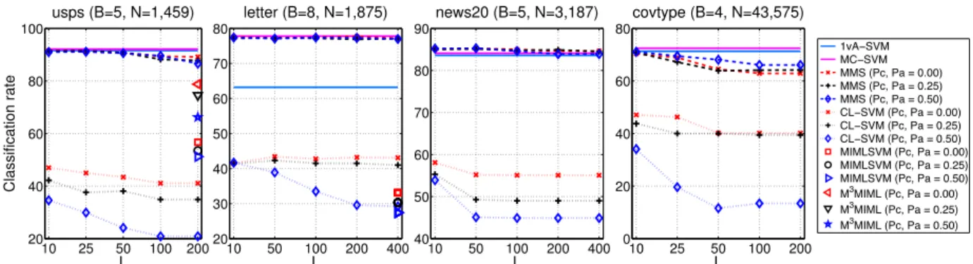
In fig. 3, we plot the average classification accuracy. Several observations can be made. First, MMS achieves results close to the supervised SVM methods, and better than all other baselines. As MMS uses a similar multi-class loss as MC-SVM, it even outperforms 1vA-SVM when the loss has its advantage (e.g. on the ‘letter’ dataset). For the ‘covtype’ dataset, the performance gap between MMS and SVM is more visible. It may due to the fact that ‘covtype’ is a class unbalanced dataset, where the two largest classes (among seven) dominate the whole dataset (more than 85% of the total number of samples). Second, the change in performance of MMS is small when the size of the candidate labeling set grows. Moreover, when correlated instances and extra noisy labels are present in the dataset, the baseline methods’ performance drops significantly, whereas MMS is less affected.
The CCCP algorithm usually converges in 3 – 5 rounds, and the final performance is about 5% – 40% higher compared to the results obtained after the first round, especially when L is large. This behavior also proves that approximating the second max(·) function in the loss function (2) with the average over all the 2. We used the original implementation at http://lamda.nju.edu. cn/data.ashx#code. We did not compare against MIMLBOOST [45], because it does not scale to all the experiments we conducted. Besides, MIMLSVM [45] does not scale to data with high dimensional feature vectors (e.g., news20 which has a 62,061-dimensions features). Running the MATLAB implementation of M3MIML [44] on problems with more than a few thousand samples is computational infeasible. Thus, we will only report results using this two baseline methods on small size problems, where they can be finished in a reasonable amount of time.
possible labeling vectors can lead to poor performance.
6
R
EAL CASE1: W
HO IS IN THE PICTURE?
The first real-world problem we tackle is naming faces in news images accompanied by captions written by journalists [4], [26]. Thanks to recent developments in the computer vision and natural language processing fields, generic faces can be localized in the images using a face detector [38] and generic names can be localized in the captions using a named entity detector [1]. Be-cause the names of the most important persons in the image typically appear in the caption, we can attempt toautomaticallylabel the detected faces with their correct names. This enables to gather a large and realistic face dataset as well as learning face classifiers directly from news items, saving the effort of manually labeling the faces. The main challenge of this task is thecorrespondence ambiguity: there could be multiple faces in the image and/or multiple names in the caption, and not all the names in the caption appear in the image, and vice versa. Some of the face detections can be false positives, which adds to the ambiguity. The task of an algorithm is to resolve the correspondence ambiguity, i.e. assign a name from the caption to each face in the image (or the null label if a person is not mentioned in the caption, or for false positive detections).6.1 Modeling
Since in this problem we are only interested in learning face classifiers, the model will associate at most one label (a name) to each detected face region (no other at-tributes). In practice, there can be thousands of different names in real world datasets (e.g. the whole of Yahoo! News Dataset [4]). However, users are typically only interested in the top K most frequent names, or only in a limited number of celebrities. Moreover, because of the ambiguities mentioned above, we add a label called null(this also covers for those infrequent names we do not model). In total, there areK+ 1classes, includingK
face classifiers to be learned.
For each detected face in an image we want to as-sign a name from the caption to it, or null. To format this problem into our framework, we use the following constraints to generate the CLSs:
• [A] a face can be assigned to exactly one name or
tonull;
• [B] a name can be assigned to at most one face; • [C] a face can be assigned only to a name appearing
in the caption of the corresponding image;
• [D] if spatial indicators, such as “left” and “(L)”,
exist, the labeling vectors in the CLSs should respect them.
In our setup, constraints [A], [B] and [C] apply to all news items, whereas constraint [D] applies only to a few items. When including constraints [A]-[C], the number of admissible candidate labeling vectors for
10 25 50 100 200 20 40 60 80 100 L Classification rate usps (B=5, N=1,459) 10 50 100 200 400 20 30 40 50 60 70 80 L letter (B=8, N=1,875) 10 50 100 200 400 40 50 60 70 80 90 L news20 (B=5, N=3,187) 10 25 50 100 200 0 20 40 60 80 L covtype (B=4, N=43,575) 4 5 6 10 20 30 40 50 60 70 80 90 100 1vAïSVM MCïSVM MMS (Pc, Pa = 0.00) MMS (Pc, Pa = 0.25) MMS (Pc, Pa = 0.50) CLïSVM (Pc, Pa = 0.00) CLïSVM (Pc, Pa = 0.25) CLïSVM (Pc, Pa = 0.50) MIMLSVM (Pc, Pa = 0.00) MIMLSVM (Pc, Pa = 0.25) MIMLSVM (Pc, Pa = 0.50) M3MIML (Pc, Pa = 0.00) M3MIML (Pc, Pa = 0.25) M3MIML (Pc, Pa = 0.50)
Fig. 3. (Best seen in color) Classification performance of different algorithms on artificial datasets.
an image-caption pair with Mi faces and Wi names is Li =Pmin(Mi,Wi) j=0 Mi j · Wi j
(see fig. 4 for an example withMi=Wi= 2). In addition, when a spatial indicator
is available, we remove the labeling vectors which do not comply with it. Take fig. 2 for example: we decide the relative position of faces by the horizontal coordinate of their center. With the spatial indicators, we know that the face in the middle can only be Grant Hackett. Then the face on the left can either be Igor Chervynsky or Erik Vendt (and the same for the face or the right). Their CLS can be generated as the two persons and two faces case. Different from previous methods, we do not allow the labeling vector which assigns all faces to null, because classifying every face as null would lead to the trivial solution with0 loss.
6.2 Inference
As stated above, searching for Zˆ in line 4 of Algo-rithm 2 is the most expensive step of the training procedure. Here we propose an algorithm which can find Zˆ efficiently. We first compute the classification scoressw(xm, y)for every instances in the bag and every
possible label y∈Y. After the scores are computed, we
use Algorithm 3 to find Zˆ in polynomial time with a bounded number of iterations.
The design of Algorithm 3 is motivated by the A∗ search algorithm [9]. The algorithm first ranks the pos-sible predictions ym for each facexmaccording to their
scoressw(xm, ym) + ∆A(y,Z(m)), whereZ(m)is them
-th row of Z. Lines 9-14 of the algorithm guarantee that all elements in the heap H have a higher score S than any S(X,Z) = Pxm∈X,zm∈Zsw(xm, zm) for any other
arbitrary compositions ofZwithzm∈Y, which not have
been added intoH. It is easy to verify that the algorithm terminates in at most L+ 1 iterations, where L is the number of candidate labeling vectors in Z. The worst case scenario is when the firstLZ¯s returned by the heap
(line 8) all belong to Z. As typically L K, the worst case complexity of searching forZˆusing Algorithm 3 is
O(L∗M), whereM is the number of regions in an image. Hence, Algorithm 3 can be used to obtaineZˆefficiently when the value of L and B is not very large (L ≤104
and M ≤10), which is the case in this task.
Algorithm 3 Efficient Algorithm for Searching forZˆ 1: input: Z, s(xm, y) + ∆A(y,Z(m)), ∀ m =
1, . . . , M, y ∈ Y
2: initialize:H = newheap, index variablejm= 1, ∀m
3: SetXmas a sorted array ofyin descending order, accord-ing tos(xm, y) + ∆A(y,Zm), ∀y∈Y 4: SetZ=ˆ X1(j1), . . . ,XM(jm)˜ 5: SetS=P ms(xm,Z(m)) 6: PushA={j=ˆ j1, . . . , jM ˜ , Z, S}intoH 7: repeat
8: PopA={j,Z¯, S}with the highest scoreS out ofH 9: form= 1,2, . . . , M do 10: Setj0 =j, thenj0 (m)++ 11: SetZ0 =ˆ X1(j0 (1)), . . . , XM(j0(M)) ˜ 12: SetS=P m0s(xm0,Z0(m0))} 13: PushA0 ={j0 , Z0 , S}intoH 14: end for 15: untilZ¯∈ Z/ 16: output: Zˆ=Z¯
In general, Algorithm 3 can not guarantee to find an exact solution Zˆ to the problem arg maxZ¯∈Z/ U(Z¯) = arg maxZ¯∈Z/ ∆A(Z,¯ Z+wt·Φ(Xk,Z¯)), denoted byZˆ∗,
at every round. This is because the algorithm only considers∆A(y,Z(m)) = 1 for those labels that do not appear in theZ(m). Let us consider a more concrete ex-ample: assume a bag{x1,x2}with two labeling vectors
z1= [1,2]andz2= [2,1]. We also know thats(x1,1) = 3,
s(x1,2) = 2, s(x1,3) = 1, s(x2,1) = s(x2,2) = 1 and
s(x2,3) = 0.99. In this case, the solution obtained by
Algorithm 3 is Zˆ = [1, 3], but Zˆ∗ = [1,1]. Despite
that, the algorithm will still obtain a Zˆ whose value of U(Zˆ) is very close to U(Zˆ∗). However, in practice,
the algorithm works very well, and the above special case rarely happens. Experiments on the same dataset show that Algorithm 3 almost always find Zˆ∗, and
that MMS executed with Algorithm 3 achieves the same performance as using an exponential time exact inference algorithm.
6.3 Experiments
We conducted experiments on the Labeled Yahoo! News dataset [4], [26]. The dataset was introduced by Berg et al. [4], and was collected from http://news.yahoo.com/. It consists of news images and their captions describing
the events appearing in the images. Guillaumin et al. [26] provides ground-truth annotations of the dataset and precomputed feature descriptors of the faced detected by [38]. The descriptors are 128-D SIFT [33] at 3 scales at 13 landmark points localized by [16], resulting in a 4992-D descriptor. In our experiments, we only use the first 1664-D features at scale 1.
We compare our results to the same baselines pro-posed in sec. 5. In MIMLSVM, null faces are automat-ically considered as negative instances. In addition, we also compare with a baseline which does not consider the appearance of the faces:
RANDOM: randomly assign a name (or null) from the caption to each face in the corresponding image.
The dataset contains 20071 images and 31147 detected faces. The maximum number of detected faces in an image is 15, and the maximum number of names in a caption is 9. There are more than 10000 different names. We consider two different protocols, detailed in the following sections:
6.3.1 Protocol I.
In the first set of experiments, we use only constraints [A]-[C] to generate the CLS Zi of each image-caption
pair. We retain the 214 names occurring at least 20 times, and treat the other names asnull. The experiments are performed over 5 different random train/test splits, sampling 80% of the items as training set and using the rest for testing. During splitting we also maintain the ratio between the number of samples from each class in the training and test set. Performance is measured by how many faces in the test set are correctly labeled with their name (or null). Moreover, we also compute name assignment performance on the training set by testing the final model on it.
Table 1 reports the name assignment performance on the training set. All the weakly supervised learning algo-rithms which consider face appearance outperform the RANDOM baseline, and MMS achieves the best result among all approaches. Table 2 summarizes the general-ization performance on the test set. Several observation can be made. First, MMS achieves performance compa-rable to the fully-supervised SVM algorithms (1vA-SVM, MC-SVM), and it outperforms the other methods which train from ambiguously labeled data (i.e. the captions). MMS even achieves an accuracy 4% higher than 1vA-SVM. This gain may be due to the fact that MMS uses a similar multi-class loss as MC-SVM, whose formula-tion is advantageous on this dataset. Moreover, we also present the result of MC-SVM trained on only half of the training data (MC-SVM[50%]), while evaluating on the same test set. The result shows that when MMS has more training data, it even outperforms the best fully supervised learning method we consider. This illustrates the promise of our method, as large amounts of image-caption pairs can be easily obtained from the internet, without manual labeling efforts.
6.3.2 Protocol II.
Here we consider all four constraints including the spa-tial indicators [D] (sec. 6.1). Only 3105 image-caption pairs contain any spatial indicator. We use all of them as part of the training set. In addition, we also randomly sample 6895 image-caption pairs from the dataset, re-sulting in a training set of 10000 image-caption pairs. All other image-caption pairs form the test set. We retain the 460 names occurring at least 3 times, and treat the other names asnull.
The results are reported in table 3 and 4. Our MMS algorithm can take advantage of the spatial indicators, and improve performance for both name association on the training set (+3.8%) and face recognition on the test set (+1.4%).
7
R
EAL CASE2: W
HO IS DOING WHAT?
The second real-world problem we tackle is finding out “who’s doing what”, i.e. associating names and action verbs in the captions to the faces and body poses of the persons in the images. In addition, the algorithm should also learn visual appearance models for the face and pose classes jointly. This task generalizes the work described in the previous section by considering the subject-verb language construct and by modeling names and verbs jointly. In our previous work [29], we have shown that the correspondence ambiguity is reduced by jointly modeling face and pose together using a generative model. In this section, we show that our MMS technique can be used to model the same problem, and achieves better performance than [29].
7.1 Modeling
In this task, the corpus of news items contains still images of persons performing actions. Each image is annotated with a caption describing “who’s doing what” in the image (fig. 1). The interesting regions in the images are persons. A person corresponds to a face and upper-body (including false positive detections), which can be detected with available software. A face and an upper-body are considered to belong to the same person if the face lies near the center of the upper-body bounding-box. One could use a named entity detector [1] and a language parser [13] to extract a list of name-verb pairs from each caption, to represent the connection between a subject and its verb in a sentence. If a name is not connected to any verb, the pair is name-null. Our system models two types of words jointly, and the goals are to: (i) associate the persons in the images to the name-verb pairs in the captions, and (ii) learn a visual appearance model for each name and each verb, corresponding to face and pose classes. These can be used for recognition on new images with or without caption.
The candidate labels for a detected person are the name-verb pairs in the caption. One label assigns a name to a face, and its connected verb from the caption to the
TABLE 1
Protocol I -Overall name assignment accuracy on the training set
Method RANDOM CL-SVM MIMLSVM MMS
Accuracy 73.1%±0.0 86.3%±0.1 89.62%±0.2 91.86%±0.3
TABLE 2
Protocol I - Overall face recognition accuracy on the test set
Supervised Learning Weakly supervised Learning
Method RANDOM 1vA-SVM MC-SVM MC-SVM[50%] CL-SVM MIMLSVM MMS
Accuracy 66.0%±0.0 81.6%±0.6 87.2%±0.3 83.3%±0.2% 76.9%±0.2 74.7%±0.9 85.7%±0.5
TABLE 3
Protocol II -Overall name assignment accuracy on the training set
Without POS With POS
Method RANDOM MMS RANDOM MMS
Accuracy 37.0%±0.0 85.3%±0.7 70.8%±0.0 89.1%±0.7
TABLE 4
Protocol II - Overall face recognition accuracy on the test set
Method RANDOM 1vA-SVM MC-SVM MMS (Without POS) MMS (With POS)
Accuracy 39.5%±0.0 82.2%±0.2 87.3%±0.1 83.5%±0.4 84.9%±0.5 Z1 Z2 Z3 Z4 Z5 Z6 Z: na na ◦ nb ◦ nb va va ◦ vb ◦ vb nb ◦ nb na na ◦ vb ◦ vb va va ◦ ← person1-face ← person1-pose ← person2-face ← person2-pose
Fig. 5. CLVs generation for the new item in fig. 1 (left). There are two detected persons,person1andperson2, and two name-verb pairs, Barack Obama-Waving (na-va) and Michelle
Obama-Standing (nb-vb). The CLVs are generated using constraints
[A]-[C] as in sec. 6.1. Labels such as Barack Obama-Standing is not allowed, as Barack is not the subject of the verb “standing” in the caption.
body pose of the same person in the image. Hence, name and verb are seen as two attributes of the same image region (a person). Therefore, during learning, to find the best possible Z ∈ Z for the image, the names and the verbs are considered jointly in making decisions. The chosen name-verb pair is the one which has the highest confidence score over both attributes. For generating constraints, we assume again the uniqueness of each person and her name and apply constraints analog to sec. 6.1 for generating the CLVs (except [D], as spatial indicators are not available in the dataset we perform experiments on). More precisely, the face and name in constraints [A]-[C] are replaced bypersonandname-verb. In this way, each person region is associated with two attributes: name and verb, which must come from the same pair detected from the caption. Fig. 5 illustrates how the CLVs are generated on an example with two persons in the image and two name-verb pairs in the caption (news item in fig. 1 (left)).
7.2 Inference
We can use Algorithm 3 to compute Zˆ. 7.3 Experiments
We conducted experiments on the Idiap/ETHZ Faces and Poses dataset3. It contains 1703 image-caption pairs collected by querying Google-images using keywords generated by combining different names (sport stars and politicians) and verbs (from sports and social in-teractions). An example query is “Barack Obama” + “shake hands”. Captions contain the names of some of the persons in the corresponding image, and verbs indicating what they are doing. The captions are derived from the snippet of text returned by Google-images and typically mention the action of at least one person in the image, but also contain names/verbs not appearing in the image. Faces and upper-bodies detected by the methods of [21], [35] were released with the dataset, so we use them directly in our experiments. We also use the available ground-truth name-verb pairs from the captions (instead of running an NLP tool).
For each person region, we extract a face descriptor a body pose descriptor. We describe the face with the method of [16], which detects nine distinctive feature points within the face bounding box. Each point is represented by the pixels in an elliptical region around it, normalized for local photometric invariance. For de-scribing the body poses, we use the features of [20]. A poseEconsist of a distribution over the position (spatial and orientation) for each of 6 body parts (head, torso, upper/lower left/right arms) output by the estimator of [15]. Three low-dimensional descriptors are derived fromE (e.g. the relative position between pairs of body parts).
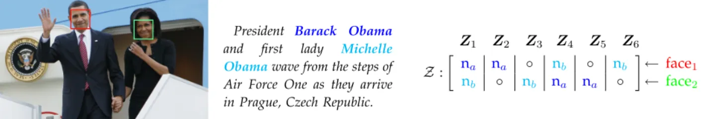
President Barack Obama
and first lady Michelle
Obamawave from the steps of Air Force One as they arrive in Prague, Czech Republic.
Z1 Z2 Z3 Z4 Z5 Z6 Z: na na ◦ nb ◦ nb nb ◦ nb na na ◦ ← face1 ← face2
Fig. 4. (Left): An example image and its associated caption. There are two detected facesface1andface2and two names Barack
Obama (na) and Michelle Obama (nb) from the caption. (Right): The CLS for this image-captions pairs. The labeling vectors are
generated using the constrain [A], [B] and [C], where thenullclass is denoted as◦.
We use non-linear kernels for both face and pose descriptors, in the form k(x,x0) = exp −γ−1d(x,x0),
with d the distance between two descriptors, and γ
selected by cross-validation. We measure the distance between two face descriptors x,x0 using d
face(x,x0) =
1−xTx0/( kxkkx0
k). In [20], different similarity measures are proposed for each type of descriptor. We normalize the range of each similarity to [0,1], and denote their average as spose(x,x0). The final distance between two poses isdpose(x,x0) = 1−spose(x,x0). The face and pose kernel matrices are computed in advance to speed up the learning. It is easy to verify that they are all Mercer kernels.
We compare the results of MMS against (i) a simplified version of the constrained mixture model “GMM” [4, sec. 2.3] which does not incorporate a language model of the caption; (ii) the distance-based generative model “DIST” [29]; (iii) a “RANDOM” baseline which ran-domly assigns a name-verb pair from the captions to each region in the corresponding image. We did not com-pare to the other weakly-supervised learning baselines used in sec. 5 & 6 because they do not support multiple attributes. As in the protocol of [29], we use 1600 items for training and 103 for testing.
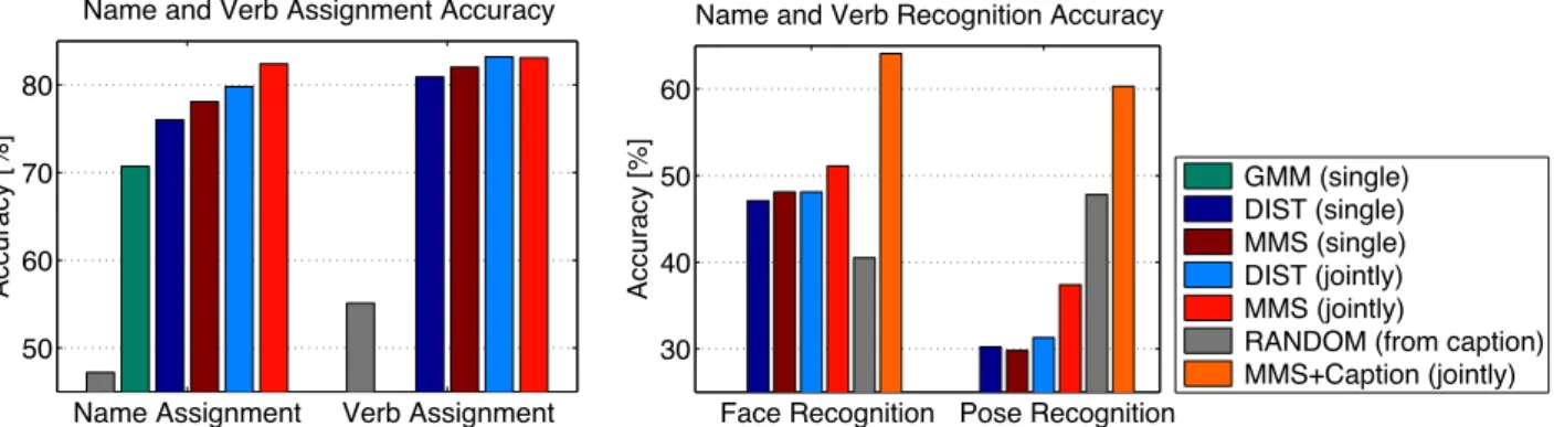
Fig. 7.3 (left) reports the name and verb assignment performance on the training set, while fig. 7.3 (right) reports the recognition results on the test images. We observe that: (i) DIST using only face information out-performs GMM for name-to-face assignment on the training set. This validates the quality of the distance-based appearance model of [29]. We reuse it also in our MMS framework. (ii) MMS outperforms DIST on both the training and the set set. (iii) the joint “face and pose” model outperforms models using face or pose information alone, demonstrating that modeling both attributes jointly reduces the correspondence ambiguity on the training set and leads to appearance models which perform better on the test set. This phenomenon holds for both DIST and MMS. (iv) on the test set, MMS gets further performance gains when given captions. In this case the problem is easier because the correct label for a person is one of the few appearing in the caption.
8
C
ONCLUSIONS AND FUTURE WORKIn this paper, we casted the problem of learning from images with captions into a new weakly supervised
learning framework. In this framework, each training sample is a bag containing multiple instances, associated with a set of candidate labeling vectors. Each labeling vector encodes the possible labels for the instances in the bag, with only one being fully correct. Our framework provides a principled way to encode different constraints widely used in many tasks, as a list of possible labelings which can be generated automatically from the image-caption pair. We also propose a large margin discrimina-tive learning algorithm to train the classifier effecdiscrimina-tively. We demonstrate on two real-world tasks that the pro-posed method can learn face classifiers from images with captions, and can learn multiple attributes jointly (names and verbs).
Our framework can be extended in several ways to solve other tasks which are not demonstrated here. For example, the popular ‘image annotation’ task: learn visual classifiers for image regions produced by unsuper-vised segmentation, from images with tags correspond-ing to nouns [3], [41]. In this task, the size of the can-didate labeling set of an image depends exponentially on the number of segments and tags. Therefore, it can be expensive to enumerate all the possible candidate labeling vectors and to inferZˆ. In this case, we could use approximate inference to speed up the learning [22]. A recent study on image annotation by Wang and Mori [41] (done independently from ours [30] in the same period) models the problem using the latent SVM framework, and formulates its inference step as a Linear Program (LP) with constraints on tags assignment. It is possible to use a similar LP formulation in our algorithm to perform the inference step approximately without enumerating all the possible assignments.
Acknowledgements:The Labeled Yahoo! News dataset were kindly provided by Matthieu Guillaumin and Jakob Verbeek. We also thank Hugo Penedones for useful discussion on the inference algorithms.
R
EFERENCES[1] http://opennlp.sourceforge.net/.
[2] S. Andrews, I. Tsochantaridis, and T. Hofmann. Support vector machines for multiple-instance learning. InProc. NIPS’03. [3] K. Barnard, P. Duygulu, D. Forsyth, N. de Freitas, D. Blei, and
M. Jordan. Matching words and pictures. Journal of Machine Learning Research, 3:1107–1135, 2003.
[4] T. Berg, A. Berg, J. Edwards, and D. Forsyth. Who’s in the picture? InProc. NIPS’04.
![Fig. 1. (Left, Middle) Two examples of image-caption pairs for the “who is doing what” task [29]](https://thumb-us.123doks.com/thumbv2/123dok_us/1364961.2682730/5.892.341.824.83.271/fig-left-middle-examples-image-caption-pairs-doing.webp)