Open Research Online
The Open University’s repository of research publications
and other research outputs
Characterization of a Highly Biodiverse Floodplain
Meadow Using Hyperspectral Remote Sensing within a
Plant Functional Trait Framework
Journal Item
How to cite:
Punalekar, Survarna; Verhoef, Anne; Tatarenko, Irina V.; van der Tol, Christiaan; Macdonald, David M.J.;
Marchant, Benjamin; Gerard, France; White, Kevin and Gowing, David (2016). Characterization of a Highly Biodiverse
Floodplain Meadow Using Hyperspectral Remote Sensing within a Plant Functional Trait Framework. Remote Sensing,
8(2) p. 112.
For guidance on citations see FAQs.
c
2016 The Authors
Version: Version of Record
Link(s) to article on publisher’s website:
http://dx.doi.org/doi:10.3390/rs8020112
Copyright and Moral Rights for the articles on this site are retained by the individual authors and/or other copyright
owners. For more information on Open Research Online’s data policy on reuse of materials please consult the policies
page.
Article
Characterization of a Highly Biodiverse Floodplain
Meadow Using Hyperspectral Remote Sensing within
a Plant Functional Trait Framework
Suvarna Punalekar1,*, Anne Verhoef1, Irina V. Tatarenko2, Christiaan van der Tol3, David M. J. Macdonald4, Benjamin Marchant4, France Gerard5, Kevin White1 and David Gowing2
1 Department of Geography and Environmental Science; School of Archaeology,
Geography and Environmental Science, The University of Reading, Whiteknights, PO Box 227, Reading RG6 6AB, UK; [email protected] (A.V.); [email protected] (K.W.)
2 Department of Environment, Earth and Ecosystems, Open University, Milton Keynes MK7 6AA, UK; [email protected] (I.V.T.); [email protected] (D.G.)
3 Department of Water Resources, Faculty of Geo-Information Science and Earth Observation (ITC), University of Twente, Enschede 7500 AE, The Netherlands; [email protected]
4 British Geological Survey, Wallingford, Oxfordshire OX10 8BB, UK; [email protected] (D.M.J.M.); [email protected] (B.M.)
5 Centre for Ecology and Hydrology, Wallingford, Oxfordshire OX10 8BB, UK; [email protected] * Correspondence: [email protected]; Tel.: +44-0749-752-0550
Academic Editors: Clement Atzberger and Prasad S. Thenkabail
Received: 5 December 2015; Accepted: 28 January 2016; Published: 3 February 2016
Abstract:We assessed the potential for using optical functional types as effective markers to monitor changes in vegetation in floodplain meadows associated with changes in their local environment. Floodplain meadows are challenging ecosystems for monitoring and conservation because of their highly biodiverse nature. Our aim was to understand and explain spectral differences among key members of floodplain meadows and also characterize differences with respect to functional traits. The study was conducted on a typical floodplain meadow in UK (MG4-type, mesotrophic grassland type 4, according to British National Vegetation Classification). We compared two approaches to characterize floodplain communities using field spectroscopy. The first approach was sub-community based, in which we collected spectral signatures for species groupings indicating two distinct eco-hydrological conditions (dry and wet soil indicator species). The other approach was “species-specific”, in which we focused on the spectral reflectance of three key species found on the meadow. One herb species is a typical member of the MG4 floodplain meadow community, while the other two species, sedge and rush, represent wetland vegetation. We also monitored vegetation biophysical and functional properties as well as soil nutrients and ground water levels. We found that the vegetation classes representing meadow sub-communities could not be spectrally distinguished from each other, whereas the individual herb species was found to have a distinctly different spectral signature from the sedge and rush species. The spectral differences between these three species could be explained by their observed differences in plant biophysical parameters, as corroborated through radiative transfer model simulations. These parameters, such as leaf area index, leaf dry matter content, leaf water content, and specific leaf area, along with other functional parameters, such as maximum carboxylation capacity and leaf nitrogen content, also helped explain the species’ differences in functional dynamics. Groundwater level and soil nitrogen availability, which are important factors governing plant nutrient status, were also found to be significantly different for the herb/wetland species’ locations. The study concludes that spectrally distinguishable species, typical for a highly biodiverse site such as a floodplain meadow, could potentially be used as target species to monitor vegetation dynamics under changing environmental conditions.
Keywords:MG4 community; field spectroscopy; optical functional types; radiative transfer model; biophysical parameters; sedge and rush
1. Introduction
Floodplain meadows are highly biodiverse and sensitive ecosystems supporting numerous species of flora and fauna [1,2]. They also provide a wide range of ecosystem services [3], such as buffer zones during flooding and are an ideal habitat for pollinating insects such as bees. Historically in the British landscape, they were mainly used for hay production and grazing. However, with changes in agricultural policies and also as a result of rapid urbanization, there has been a sharp decline in the area covered by floodplain meadows [4,5]. In particular, the biodiversity of these meadows is under constant threat due to changes in hydrological regime, poor management and agricultural intensification. Because of their high ecological significance, they have been given a high conservation priority, and hence they need to be studied and monitored closely to prevent any further loss of biodiversity.
Being complex ecosystems with delicate interlinkages between vegetation, hydrological and nutrient regimes, floodplain meadows are important sites for studying ecosystem behavior under changing climatic conditions. Although there has been an increase in scientific research on floodplain meadows in recent years, most of the literature is based on time- and labor-intensive conventional methods, such as botanical surveys (for example, [1,2,6]). Integration of these methods with modern technologies can lead to more efficient ways to study and monitor these complex ecosystems. Vegetation spectral data, for instance, provide a promising means to monitor the biodiversity as well as vegetation quality, quantity and dynamics (e.g., [7,8]).
In ecological research, applications of remote sensing data can be grouped into three categories. Firstly, mapping vegetation cover is done by relating vegetation types to spectral data and from that sub-community or species level maps are generated [9,10]. Recently, this application has also been extended to mapping biodiversity by correlating spectral variations with species richness or abundance [11,12]. The second category of applications derives empirical relationships between spectral data and vegetation biophysical and biochemical properties such as total biomass, leaf pigments or water content, thereby improving our understanding of the physiological conditions of the vegetation [13–17]. Finally, there are applications that use remotely sensed vegetation properties in ecosystem models to understand functional dynamics such as evapotranspiration and photosynthesis [18–21].
Modern hyperspectral sensors have opened a vast area of research for analyzing species-level differences in biophysical and chemical properties [22–27]. With the availability of fine resolution datasets and advanced knowledge about vegetation and environment interactions, the focus of remote sensing applications in ecological research is gradually shifting towards utilizing spectral data to characterize vegetation into functional types [25,28–31]. This involves integrating all three kinds of applications discussed above, wherein observed spectral differences are explained with respect to biochemical and structural differences in the vegetation and these differences are then related to the functional interactions between vegetation and its environment. Although there is no universally accepted single definition of functional type, it involves “grouping species based on their structural, physiological and/or phenological features in response to environmental conditions or according to their impacts on ecosystem” [29]. Thus, the monitoring of functional types may help predict changes in vegetation with respect to changes in their immediate environment [32–35]. However, the concept of “functional types” is still largely context dependent due to the occurrence of a wide range of physiological, morphological and biochemical traits, which make a discrete classification virtually impossible. Furthermore, multiple approaches exist to classify vegetation into functional types based on ecological, botanical or modeling points of view [29]. Thus, it is important to assess which of these
functional types are distinguishable in spectral data. From a spectroscopy perspective there are a limited number of useful functional traits such as leaf pigment content, leaf dry matter, water content, Leaf Area Index (LAI), and leaf angle distribution; these all play an important role in radiative transfer and hence govern vegetation spectral behavior [13,36,37]. Thus, they can potentially be used to study functional differences in the target ecosystems through spectroscopy [29,36,38,39]. This has further led to the concept of ”optical functional types”, which refers to vegetation functional types that could be traced using spectral datasets [28,29].
Despite these developments, applications to study herbaceous communities are still limited. These communities, in general, are very challenging for spectroscopy research [38] due to the relatively small plant size and the presence of an often diverse assemblage of species and multiple plants in one sampling unit. There have been applications of remote sensing to herbaceous communities, such as those monitoring species diversity (e.g., [32,40–42]) involving retrieval of properties such asLAIand biomass using empirical methods or radiative transfer model inversion [43–46]. However, there is a recognized need for further research on spectroscopy-based vegetation biophysical and functional characterization [47,48].
In this paper, we investigate the potential for and limitations of spectral data in characterizing important optical functional types in a typical UK floodplain meadow community. We assess if it is possible to identify spectrally distinguishable members of the community. We investigate if their leaf and canopy level biophysical and biochemical properties explain the observed differences in vegetation spectra with the help of radiative transfer model. With the help of these properties and some additional functional traits, we explain the functional differences in the optical types. We have also monitored groundwater level and soil available nitrogen to understand differences in the water and nutrient availability in root zone of these optical types. Thus, we assess the potential of optical functional types to be used as effective markers to monitor changes in vegetation in floodplain meadows and associate them with changes in their immediate environment.
2. Background
2.1. MG4 Floodplain Meadows
In the UK, floodplain meadow communities are described using the National Vegetation Classification (NVC). The meadow used within this study is classified as MG4 [49], which at the European scale forms part of the “Alopecurionalliance” [50]. MG4 isAlopecurus pratensis–Sanguisorba officinalisgrassland (syn.Fritillario–Alopecuretum pratensiswith 16 constant species referring to those that are typical members of MG4) including grasses and broad leaf herbaceous species. It is one of the most typical floodplain communities in the UK; a semi-natural ecosystem developed as a result of traditional management. This management allows vegetation to grow during spring and summer, which is then cut for hay during June–July, followed by grazing in the two months in early autumn. The hay harvest removes nutrients from the meadows and replacement is primarily via surface water flooding. Nutrient status is then dependent on a combination of groundwater flows, soil-moisture and related soil aeration status, and soil temperature; changes in hydrological regime can significantly alter nutrient availability [1]. The meadow soils often have low nutrient availability, which limits plant growth. This limitation increases the competition between plant species and prevents dominance of the community by any aggressive species, contributing to the high levels of diversity in the plant community [2,49]. This community can consist of many grass and broad leaf herbaceous species as well as several sedges, rushes, ferns and mosses with total numbers of species reaching 40 per square meter. The MG4 community is found on soil that can supply enough water during the growing season and also supports adequate aeration, and is more negatively affected by water logging than by water scarcity [1,2]. On drier soils the MG4 shows transitions towards MG5 community, which has a dominance of dry indicator species such asCenturea nigraandLeucanthemum vulgare; on wetter soils it moves towards MG8 (Cynosurus cristatus–Caltha palustrisgrassland; [2]) or shows dominance
of species likeFilipendula ulmaria or even wetland species. It is important to note that the NVC system is based on the association of species; it does not directly take into account the soil moisture, nutrient or hydrological conditions. However, extensive research has been carried out to associate the communities with water availability in soil by defining preferred ranges of water table depth through long-term groundwater level (GWL) and botanical surveys [1,2,51].
2.2. Study Area
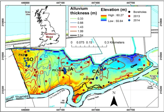
The field site, known as Yarnton Mead, has an area of 32 ha, and is located on the floodplain of the River Thames (Figure1), northwest of the city of Oxford [52] in the lowlands of southern UK (51.791499N,´1.296714E). It forms part of the Oxford Meadows, an EU designated Special Area of Conservation. The site is relatively flat with elevation ranging between 55 and 60.3 m and has a shallow water table, typically fluctuating within 0.6 m of the ground surface. Depth to groundwater is determined by a number of factors: proximity to the River Thames, which, due to a downstream weir, has a consistently high water level causing recharge to the gravel aquifer along the whole of its reach adjacent to the meadow; proximity to ditches, primarily the ditch that runs along the north of the meadow, which is both a discharge line and a route for flood waters; but mainly due to the topography, with low-lying zones more prone to waterlogging. The meadow is underlain by alluvial deposits: a fine-grained alluvium of silts, clays and fine-to-medium sand of variable thickness, over calcareous gravel. The predominant soil type is a silty clay loam with an organic top layer of variable thickness. A map of thickness of alluvium was derived for Yarnton Mead from a surface geophysical survey using an EM31ground conductivity meter (Geonics Ltd., Mississauga, ON, Canada). Typical representative species of MG4 and species representing its transition towards MG5 (discussed in Section2.1) occur mainly in the northwest of the meadow, an area of the field characterized by relatively thin alluvium. Wetness-indicating species are coincident with the low-lying areas and with areas of thick clayey alluvium that have poor drainage (Figure1). Although alluvium thickness may not directly govern species composition, it plays a role by modulatingGWL.
Remote Sens. 2016, 8, 112
4
to associate the communities with water availability in soil by defining preferred ranges of water table depth through long-term groundwater level (GWL) and botanical surveys [1,2,51].
2.2. Study Area
The field site, known as Yarnton Mead, has an area of 32 ha, and is located on the floodplain of the River Thames (Figure 1), northwest of the city of Oxford [52] in the lowlands of southern UK (51.791499N, −1.296714E). It forms part of the Oxford Meadows, an EU designated Special Area of Conservation. The site is relatively flat with elevation ranging between 55 and 60.3 m and has a shallow water table, typically fluctuating within 0.6 m of the ground surface. Depth to groundwater is determined by a number of factors: proximity to the River Thames, which, due to a downstream weir, has a consistently high water level causing recharge to the gravel aquifer along the whole of its reach adjacent to the meadow; proximity to ditches, primarily the ditch that runs along the north of the meadow, which is both a discharge line and a route for flood waters; but mainly due to the topography, with low-lying zones more prone to waterlogging. The meadow is underlain by alluvial deposits: a fine-grained alluvium of silts, clays and fine-to-medium sand of variable thickness, over calcareous gravel. The predominant soil type is a silty clay loam with an organic top layer of variable thickness. A map of thickness of alluvium was derived for Yarnton Mead from a surface geophysical survey using an EM31ground conductivity meter (Geonics Ltd., Mississauga, ON, Canada). Typical representative species of MG4 and species representing its transition towards MG5 (discussed in Section 2.1) occur mainly in the northwest of the meadow, an area of the field characterized by relatively thin alluvium. Wetness-indicating species are coincident with the low-lying areas and with areas of thick clayey alluvium that have poor drainage (Figure 1). Although alluvium thickness may not directly govern species composition, it plays a role by modulating GWL.
Figure 1. Yarnton Mead with sampling locations for 2013 and 2014, elevation map (from airborne LIDAR survey in June 2014) and alluvium thickness contour lines (Courtesy of Hanson UK), overlaid on Ordnance Survey 1:10,000 scale base-map.
Figure 1. Yarnton Mead with sampling locations for 2013 and 2014, elevation map (from airborne LIDAR survey in June 2014) and alluvium thickness contour lines (Courtesy of Hanson UK), overlaid on Ordnance Survey 1:10,000 scale base-map.
3. Materials and Methods
The field sampling was done during spring and early summer season (end of March to early July) in 2013 and 2014. This period corresponds to undisturbed and rapid vegetation growth, followed by flowering and fruiting stages of the plant life cycle. In 2013, the spectral sampling strategy was designed to capture reflectance of fully-grown species assemblages as their composition changes over the meadow with respect to the soil water availability (i.e., “sub-community based” approach). In 2014, near-homogeneous, fully-grown canopies of three species were targeted for spectral measurements (i.e., “Species based” approach). The observed spectral differences were then explained through vegetation radiative transfer model sensitivity runs and field measurements of plant optical parameters. In addition to the optical parameters, plant functional properties, and nutrient conditions in the plant root zone were studied at species level, with the aim of assessing the functional differences between the typical MG4 representative species and wetland species.
3.1. Sampling Locations
For the “sub-community based” sampling in 2013, we considered two subcategories of MG4 based on eco-hydrological differences—DRYandWET. Over the field, 25 locations (Figure1, red dots) were chosen using a Latin hypercube algorithm [53], which ensured that the variability in elevation, alluvium depth and information from an NVC map [54] was well represented. Although, through the NVC map, overall community level variability was taken into account, exact botanical composition was not known before selection of the sampling locations. Botanical surveys were carried out at these locations in mid May 2013. Based on the projective cover of indicator species in 1 m by 1 m sampling plots, the locations were assigned to aDRY orWETcategory. Table1lists species used for theDRYandWETclassification. Average score on Ellenberg’s moisture scale forDRYspecies would be 5 and forWETwould be 7.4 [55]. In general, the locations with a typical MG4 community, and those showing botanical transition towards MG5 were also grouped into theDRYclass, while others with sedges, rushes, and wetness indicating grass and herb species were grouped into theWET class. Furthermore, in addition to the 25 locations, we also included two small transects (one with 14 locations and another with 7 locations, both with roughly 5 m intervals between adjacent locations) through different vegetation patches. The species assemblages at these locations were also assigned to theDRY or WETclasses based on their botanical compositions.
Table 1. List of prominent species, grouped under vegetation classes, studied for spectral discrimination, including the final number of sampling locations (and spectra) after removal of poor-quality measurements.
Class Main Species Found Date of
Spectral Sampling
Number of Sampling Locations
DRY
Sanguisorba officinalis, Centaurea nigra, Succisa pratensis, Galium verum, Lotus corniculatus, Primula veris, Dactylis glomerata, Carex flacca, Festuca rubra, Trisetum flavescens
5 and 9 July 2013 25 (400 spectra)
WET
Carex riparia, Carex acuta, Juncus acutiflorus; Filipendula ulmaria, Thalictrum flavum,
Lysimachia numullaria, Holcus lanatus, Hordeum secalinum, Cardamine pratensis,
Agrostis stolonifera
5 and 9 July 2013 10 (158 spectra)
SO Sanguisorba officinalis 12 June 2014 8 (131 spectra)
CA Carex acuta, Carex riparia 13 June 2014 10 (146 spectra)
JA Juncus acutiflorus 12 and 13 June 2014 7 (85 spectra)
For the species based sampling in 2014, three important species were selected, namelySanguisorba officinalis (SO),Juncus acutiflorus (JA)andCarex acuta (CA). This choice was based on the following
important species-differentiating facts:SOis a herb from the Dicotyledonous Class of plants forming rosettes of oblong pinnate leaves and is a typical representative of MG4 community (Figure2a);JA, a rush, andCA, a sedge, represent the Monocotyledon Class of plants differing from the Dicots by their growth habits. Normally they are absent on MG4 meadows or occur in small amounts, however, on Yarnton Mead, they have started to dominate in wet parts of the meadow in recent years [54].JAhas almost cylindrical tube-like, glossy leaves that taper at the end to form a sharp tip (Figure2c). CA, however, has linear, glaucous leaf blades with a bluish tinge (Figure2b). On Yarnton Mead,CAoccurs in close association with another big sedge,Carex riparia; because of their similar growth habit, we grouped them together intoCA. Besides these botanical observations, the change in spectral sampling, from sub-community to species based approach, was driven also by conclusions drawn from the spectral data analysis obtained in 2013 (discussed in Section4.1.1).
Remote Sens. 2016, 8, 112
6
(Figure 2a); JA, a rush, and CA, a sedge, represent the Monocotyledon Class of plants differing from the Dicots by their growth habits. Normally they are absent on MG4 meadows or occur in small amounts, however, on Yarnton Mead, they have started to dominate in wet parts of the meadow in
recent years [54]. JA has almost cylindrical tube-like, glossy leaves that taper at the end to form a
sharp tip (Figure 2c). CA, however, has linear, glaucous leaf blades with a bluish tinge (Figure 2b).
On Yarnton Mead, CA occurs in close association with another big sedge, Carex riparia; because of
their similar growth habit, we grouped them together into CA. Besides these botanical observations,
the change in spectral sampling, from sub-community to species based approach, was driven also by conclusions drawn from the spectral data analysis obtained in 2013 (discussed in Section 4.1.1).
Figure 2. Digital photographs showing top of canopy (1 m height above ground) for (a) Sanguisorba officinalis (SO); (b) Carex acuta and Carex riparia (CA) and (c) Juncus acutiflorus (JA). Photographs taken on 12 and 13 June 2014.
We identified three areas in the field where one of the target species was most abundant (Figure 1). Next, 10–12 locations were chosen in each area based on the criteria that within a 1 m by 1 m plot around the location (marked with canes) the projective cover of the target species was more than 90% (blue dots in Figure 1) and locations are at least 5 m away from each other.
3.2. Spectral Sampling, Post Processing and Analysis
Spectral radiance in nadir direction was measured in 2013 with a SVC HR-1024 hyperspectral spectroradiometer on 5 and 9 July, and in 2014, with a slightly advanced version of the same instrument (known as SVC HR-1024i; with on-board digital camera and GPS) on 12 and 13 June. Both
spectroradiometers record the radiance for more than 900 spectral bands covering the visible (VIS),
near infrared (NIR) and short wave infrared (SWIR) regions of wavelengths, and have a similar
spectral resolution (3.5 nm in VIS, 9.5 nm in NIR and 6.5 nm in SWIR). Foreoptics with 8°
instantaneous field of view was used for spectral sampling from 1 m height above the ground,
sampling a circular ground area of 154 cm2 (i.e., a radius of 6.9 cm). Each radiance measurement was
taken with an integration time of 3 s. At each sampling location a plot of 1 by 1 m was sampled. It was divided into 16 grid-cells of equal size (~0.25 m by 0.25 m). Target measurements were taken approximately in the center of each of these 4 by 4 grid-cell configurations. Regular reference measurements, required to convert radiances into reflectance, was taken over spectralon panel before every 4 target measurements. The same measurement protocol was followed in both years. Sampling dates reflect maximum vegetative growth and predominantly clear sky conditions necessary for spectroscopy. However, not all planned locations could be sampled on each sampling date due to interruptions caused by the frequent and partial cloud cover.
The radiance data were post-processed to produce calibrated reflectance spectra ( ; subscript λ refers to wavelength) using the field spectroscopy toolbox (Field Spectroscopy Facility, http://fsf.nerc.ac.uk). This process, followed by qualitative checks using the field photographs and notes, led to further removal of spectral data that were considered sub-optimal due to poor
Figure 2.Digital photographs showing top of canopy (1 m height above ground) for (a)Sanguisorba officinalis(SO); (b)Carex acutaandCarex riparia(CA) and (c)Juncus acutiflorus(JA). Photographs taken on 12 and 13 June 2014.
We identified three areas in the field where one of the target species was most abundant (Figure1). Next, 10–12 locations were chosen in each area based on the criteria that within a 1 m by 1 m plot around the location (marked with canes) the projective cover of the target species was more than 90% (blue dots in Figure1) and locations are at least 5 m away from each other.
3.2. Spectral Sampling, Post Processing and Analysis
Spectral radiance in nadir direction was measured in 2013 with a SVC HR-1024 hyperspectral spectroradiometer on 5 and 9 July, and in 2014, with a slightly advanced version of the same instrument (known as SVC HR-1024i; with on-board digital camera and GPS) on 12 and 13 June. Both spectroradiometers record the radiance for more than 900 spectral bands covering the visible (VIS), near infrared (NIR) and short wave infrared (SWIR) regions of wavelengths, and have a similar spectral resolution (3.5 nm inVIS, 9.5 nm inNIRand 6.5 nm inSWIR). Foreoptics with 8˝instantaneous
field of view was used for spectral sampling from 1 m height above the ground, sampling a circular ground area of 154 cm2(i.e., a radius of 6.9 cm). Each radiance measurement was taken with an integration time of 3 s. At each sampling location a plot of 1 by 1 m was sampled. It was divided into 16 grid-cells of equal size (~0.25 m by 0.25 m). Target measurements were taken approximately in the center of each of these 4 by 4 grid-cell configurations. Regular reference measurements, required to convert radiances into reflectance, was taken over spectralon panel before every 4 target measurements. The same measurement protocol was followed in both years. Sampling dates reflect maximum vegetative growth and predominantly clear sky conditions necessary for spectroscopy. However, not all planned locations could be sampled on each sampling date due to interruptions caused by the frequent and partial cloud cover.
The radiance data were post-processed to produce calibrated reflectance spectra (ρλ; subscript
λ refers to wavelength) using the field spectroscopy toolbox (Field Spectroscopy Facility,
http://fsf.nerc.ac.uk). This process, followed by qualitative checks using the field photographs and notes, led to further removal of spectral data that were considered sub-optimal due to poor illumination conditions. An average reflectance spectrum for each location was calculated using all good quality spectra at that location (mostly ranging between 10 and 16 in number).
Different tests were performed using the spectral reflectance data to characterize spectral variations between the sub-community and species based vegetation classes. The average and standard deviation of each vegetation class was calculated using all locations within the class.
The discrimination metricD[56] was calculated to assess the dissimilarity in theρλmeasured
over the two sub-communities and three key species,
D“ r 1 n´1 n ÿ i“1 pρre fλ i ´ρ sam λi q 2 s 1{2 (1)
wherenis the number of wavelengths used between 400 and 2470 nm (n= 923 for year 2014 data, and 935 for year 2013 data); and superscripts “ref” and “sam” refer to reference and sample spectra, respectively. This metric enables the comparison of vegetation class pairs (for example, comparingSO withCAorWETwithDRY), with one as the reference and the other as the sample spectrum. Smaller values ofDindicate less dissimilarity between reference and sample spectra.Dwas calculated for all possible class pairs (SO–CA,SO–JA,CA–JA, andDRY–WET).
A further technique (developed by Cochrane [56]), “spectral shape filtering”, which differentiates vegetation classes based on the overall shape of their spectra, was implemented. It involves normalizing all the measuredρλ(samandref) by dividing them by a standard spectrum and evaluating the location
of the normalized spectrum ofsamrelative to the spectral shape space of the standard spectrum. The standard spectrum is the averageρλof theref class. The spectral shape space forrefclass is defined
by minimum and maximum values at each wavelength, considering all the normalized spectra ofref. If the average normalized spectra forsamfall within the spectral space ofref, it indicates thatsamis spectrally inseparable fromref.
Finally, the difference inρλwas tested for statistical significance at every wavelength between
different pairs of classes. The non-parametric ANOVA test (Mann–Whitney U test) was used for this purpose as it does not rely on the assumption of normal distribution of spectral data and compares sample median rather than mean. It has also been used in similar types of spectroscopy based research [41,57,58].
3.3. Field Data Collection for Vegetation Biophysical and Functional Properties
The canopy-level structural parameterLAIwas measured in 2013 and 2014 using the Sunscan Canopy Analysis System (Delta-T Devices, Burwell, UK). Five to seven measurements were taken below the canopy at every location. LAIwas measured within 1 to 5 days of the spectral sampling. Simultaneously with the spectral sampling on 12 and 13 June 2014, leaf samples were collected for each target species to obtain leaf chlorophyll content (Lcc), leaf dry matter content (Ldmc), leaf water content
(Lwc) and specific leaf area (SLA), using standard laboratory techniques. Leaf samples from different
locations were bulked to form a main sample. Ten leaves were drawn from the main sample for determination ofLcc. Chlorophyll content was obtained by acetone extraction method, and standard
equations [59,60] were used to convert the absorbance measurements into chlorophyll concentrations. Another set of 10 leaves was used to measure leaf area using a calibrated Delta-T leaf area meter. Once the area was measured, leaves were weighed immediately for fresh weight. They were then oven-dried at 80˝C for 48 hours, and weighed again to determineL
dmc,LwcandSLA.Lcc,LdmcandLwc
After leaf biochemical analysis, the remaining plant material was dried at 80˝C for two days,
ground into fine powder and subjected to total carbon and nitrogen analysis in a Thermo Flash 2000 Carbon Nitrogen Analyser, using aspartic acid as standard material for calibration. This analysis gave percentage of leaf nitrogen and carbon content (NlandCl) in leaf dry matter.
Along with the spectral sampling in June 2014, CO2response curves (also known asA-Ci, or
photosynthesis-intercellular CO2response curves) were also measured using a LICOR-6400 InfraRed
Gas Analyser (IRGA) to estimateVcmax(maximum carboxylation capacity of Rubisco enzyme involved
in photosynthesis) forSO,CAandJA.The protocol for these measurements was developed based on [61]. Subsequently, leaves used for determination of the response curves were cut, and their area was measured using a leaf area meter. TheA–Cicurves were corrected for actual leaf area and then
used in Curve-Fit GUI (version 0.5) to estimateVcmax[62].
The vegetation and soil available nitrogen (explained in Section3.5) have been tested for significant difference among different vegetation groups by one-way ANOVA tests using GENSTAT statistical package (v16.1.10916). When testing more than two groups (for example,SO,CAandJA) for significant difference, Fisher’s unprotectedt-test was used for pair-wise comparison. We inspected the histogram of the residuals and a plot of the expected normal quantiles against the residuals to ensure that the residuals approximated a normal distribution. Single outliers were identified amongst the measurements of dry matter and water content. These were removed prior to conducting the ANOVA. 3.4. Model Simulations
A one-by-one sensitivity analysis was conducted with the PROSAIL canopy radiative transfer model [37,63,64] to help explain the effect of each optical parameter onρλin association with the
field measurements. The PROSAIL model is a coupled canopy (SAIL) and leaf radiative transfer (PROSPECT) model that has been widely used and tested for different kinds of canopies such as agricultural crops, grasslands, and forests [37]. The model simulates canopyρλbased on information
provided about illumination and observation geometry, and vegetation and soil optical properties. The vegetation optical parameters areLAI,Lcc,Ldmc,Lwc, leaf thickness parameter (N), and a parameter
describing leaf inclination. The leaf inclination is modeled using a leaf inclination distribution function (LIDF). Within this function leaf angles are represented by parameterLIDFain PROSAIL. The value
ofLIDFavaries from´1.0 for completely erectophile to 1.0 for completely planophile leaves, but the
range from´0.5 to 0.5 covers common leaf inclinations in reality. The sensitivity analysis entailed calculation of canopyρλin the nadir direction, for different values of the six canopy optical parameters;
one parameter was varied at a time, while the others were kept constant (at representative values of LAI= 5 m2¨m´2,L
dmc= 0.008 g¨cm´2,Lcc= 30µg¨cm´2,Lwc= 0.009 cm,LIDFa=´0.35 (unitless), and
N= 1.6 (unitless)). The range of parameter values was determined based on the field data, except forN, as it could not be easily measured in absence of leaf level spectral measurements. This parameter refers to internal leaf structure, cell arrangements and intercellular air spaces [64]. Some mixed grassland studies have reported values ofNaround 1.5 to 1.7. In absence of any field-based information,Nwas varied uniformly within the wide range reported in the literature (i.e., 1.3 to 2.1). The distribution of other parameters within their respective range were chosen such that they are proportional to the sensitivity ofρλto that parameter [65].
The vegetation over the meadow was very dense and covered soil completely, thus making soil spectral parameterization less important. A typical spectrum of organic meadow soil has been used to describe soil reflectance.
3.5. Soil Measurements
Time-integrated availability of root zone soil nitrate pNO´3qand ammonium pNH`4q, hence available soil nitrogen over the study period were measured using Plant Root Simulator (PRS) probes (Western-Agsolutions, Saskatoon, SK, Canada, http://www.westernag.ca). These probes are of two types—anion and cation. They consist of ion exchange resin strips (~7 cm long and ~1 cm wide)
encased in a firm plastic frame. The total surface area of resin strips is 17.5 cm2, including both sides. They were buried vertically down in the soil so that the resin strips were completely in contact with the soil. In 2014, three locations were chosen in each of theSO, CAandJAsampling locations. At each sampling location, four pairs (anion and cation) of PRS probes were installed. Two batches were used: the first set was installed on 3 May and removed on 1 June 2014; the second batch was deployed on 1 June and removed on 4 July 2014. The probes were transported in sealed plastic bags in a cool-box and, after thorough washing in the laboratory using de-ionized water, were then sent in insulated cool-boxes to the manufacturer for analysis.
3.6. Groundwater Level Data Acquisition
In the absence of continuous monitoring of root zone soil moisture, groundwater level data (GWL) were used in the study as a proxy for soil moisture. From the existing network of 17 boreholes on the site, three were identified that coincide with the three species-dominated focus areas. The locations of these boreholes are shown in Figure1. All three boreholes are completed in the gravel aquifer with 1-metre long screens at their base. Non-vented data loggers (Rugged Troll 100,In-Situ, Fort Collins, CO, USA) installed in the boreholes measure pressure; height of the water column above the logger, and in turn the depth to groundwater, is calculated by combining total pressure with output from a barometric pressure data logger (Rugged BaroTroll,In-Situ), also located on Yarnton Mead. The loggers provide water level measurements on an hourly interval, validated by manual monitoring of water levels on a monthly basis using a water level meter (Soil Instruments, Uckfield, East Sussex, UK). 4. Results
4.1. Spectral Variations
All spectral analysis tests show that theDRYandWETsub-community based classes are spectrally very similar, while for the species based classes results suggest spectral differences betweenSOand CAorJAwith mixed results for differences betweenCAandJA. The results are elaborated further. 4.1.1. Sub-Community Based Spectral Discrimination
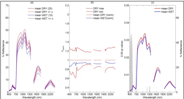
The spectral variability plot (Figure 3a) of the sub-community based approach shows that the averageρλ of theDRY class was overall slightly higher than that of theWETclass across all
wavelengths. However, the plots of the meanρλalong with standard deviation for the two groups
consistently overlapped.
The discrimination metricDwas equal to 1.66 for theDRY–WETcomparison and markedly lower than theDvalues obtained for the species-based approach (see Section4.1.2below), indicating a strong similarity betweenρλof theseDRYandWETclasses.
The shape filter analysis plot (Figure3b) shows the spectral shape space forDRY, and average spectrum ofWETnormalized with respect toDRY. The normalized spectrum ofWETwas well within the upper and lower boundary of spectral shape space forDRY. The shape filter analysis confirms the results of the metricDthatρλofWETcould not be distinguished fromDRYat any wavelength.
Finally, results of the band-wise Mann–Whitney U tests (Figure3c) also showed that the spectral differences betweenWETandDRYclass were not statistically significant over most of the measured wavelengths, except between: 400 and 541 nm; 666 and 681 nm; 719 and 728 nm; and 1165 and 1316 nm. However, in the shape filter plot, no difference was observed at these wavelengths.
Remote Sens.2016,8, 112 10 of 22
9
and, after thorough washing in the laboratory using de-ionized water, were then sent in insulated cool-boxes to the manufacturer for analysis.
3.6. Groundwater Level Data Acquisition
In the absence of continuous monitoring of root zone soil moisture, groundwater level data
(GWL) were used in the study as a proxy for soil moisture. From the existing network of 17 boreholes
on the site, three were identified that coincide with the three species-dominated focus areas. The locations of these boreholes are shown in Figure 1. All three boreholes are completed in the gravel
aquifer with 1-metre long screens at their base. Non-vented data loggers (Rugged Troll 100, In-Situ,
Fort Collins, CO, USA) installed in the boreholes measure pressure; height of the water column above the logger, and in turn the depth to groundwater, is calculated by combining total pressure with
output from a barometric pressure data logger (Rugged BaroTroll, In-Situ), also located on Yarnton
Mead. The loggers provide water level measurements on an hourly interval, validated by manual monitoring of water levels on a monthly basis using a water level meter (Soil Instruments, Uckfield, East Sussex, UK).
4. Results
4.1. Spectral Variations
All spectral analysis tests show that the DRY and WET sub-community based classes are
spectrally very similar, while for the species based classes results suggest spectral differences
between SO and CA or JA with mixed results for differences between CA and JA. The results are
elaborated further.
4.1.1. Sub-Community Based Spectral Discrimination
The spectral variability plot (Figure 3a) of the sub-community based approach shows that the
average of the DRY class was overall slightly higher than that of the WET class across all
wavelengths. However, the plots of the mean along with standard deviation for the two groups
consistently overlapped.
Figure 3. (a) Average spectra (along with standard deviation) measured in nadir direction above canopy of DRY and WET class on 5 and 9 July 2013; (b) Shape filter space of DRY class with mean of normalized (with respect to DRY) spectra of WET class vegetation; (c) Results of wavelength wise Mann–Whitney U test between WET and DRY location spectra showing significant differences in grey scale (p-value< 0.05). Number of sampling locations is given in bracket in the legend of plot 3a. Figure 3. (a) Average spectra (along with standard deviation) measured in nadir direction above canopy ofDRYandWETclass on 5 and 9 July 2013; (b) Shape filter space ofDRYclass with mean of normalized (with respect toDRY) spectra ofWETclass vegetation; (c) Results of wavelength wise Mann–Whitney U test betweenWETandDRYlocation spectra showing significant differences in grey scale (p-value < 0.05). Number of sampling locations is given in bracket in the legend of plot 3a. 4.1.2. Species-Based
Figure4a shows the averageρλforSO,CAandJAalong with their standard deviations.Reflectance
forSOwas higher than forCAandJAover almost all wavelengths, but particularly in theNIRand SWIRregion (750 to 1200 nm).SOhad the highest andJAhad the lowestρλ, withρλforCAlocated in
between. Averageρλin theNIRshoulder (700 to 750 nm) was 50%–52% forSO, 38%–40% forCAand
30%–32% forJA. However, there was considerable overlap between the mean and standard deviation spectra forJAandCA(Figure4a).
The dissimilarity matrix D was 12.21 between SO and JA, and 8.63 between SO and CA, which indicates a high dissimilarity between the mean spectrum of SOand those of CA andJA. The‘dissimilarity matrixDbetweenCAandJAwas equal to 3.67, which is less than theDbetweenSO andCAas well as betweenSOandJA.
The shape filter analysis plot (Figure4b) shows the spectral shape space forSO and average spectra ofCAandJAnormalized with respect toSO; theρnormofJAcould be discerned fromSOfor
all wavelengths. In the case ofCA,ρnormwas outside the spectral shape space ofSOfor most of the
wavelengths, except a few in theSWIRregion near 2000 nm. WhenJAspectra were normalized with respect toCA, they also fell outside the spectral shape space ofCA, but it was aligned much closer to the lower boundary of the shape space ofCAin theVISandNIRpart of the spectrum (Figure4c). The distance between this lower boundary andρnormofJAincreased in theSWIRregion.
The Mann–Whitney U tests plots show thatρλwere significantly different betweenSO–JAand
SO–CAover all the wavelengths (Figure4d,e). In the case ofCA–JA,ρλwas also significantly different
Remote Sens.2016,8, 112 11 of 22
10
The discrimination metric D was equal to 1.66 for the DRY–WET comparison and markedly lower than the D values obtained for the species-based approach (see Section 4.1.2 below), indicating a strong similarity between of these DRY and WET classes.
The shape filter analysis plot (Figure 3b) shows the spectral shape space for DRY, and average spectrum of WET normalized with respect to DRY. The normalized spectrum of WET was well within the upper and lower boundary of spectral shape space for DRY. The shape filter analysis confirms the results of the metric D that of WET could not be distinguished from DRY at any wavelength.
Finally, results of the band-wise Mann–Whitney U tests (Figure 3c) also showed that the spectral differences between WET and DRY class were not statistically significant over most of the measured wavelengths, except between: 400 and 541 nm; 666 and 681 nm; 719 and 728 nm; and 1165 and 1316 nm. However, in the shape filter plot, no difference was observed at these wavelengths.
4.1.2. Species-Based
Figure 4a shows the average for SO, CA and JA along with their standard deviations.
Reflectance for SO was higher than for CA and JA over almost all wavelengths, but particularly in the
NIR and SWIR region (750 to 1200 nm). SO had the highest and JA had the lowest , with for
CA located in between. Average in the NIR shoulder (700 to 750 nm) was 50%–52% for SO, 38%–40% for CA and 30%–32% for JA. However, there was considerable overlap between the mean and standard deviation spectra for JA and CA (Figure 4a).
Figure 4. (a) Average spectra (along with standard deviation) measured in nadir direction above canopy of SO, CA and JA on 12 and 13 June 2014;(b) Shape filter space of SO class with mean of normalized spectra (with respect to SO) of CA and JA; (c) Shape filter space of CA class with mean of normalized (with respect to CA) spectra of JA; (d–f) Results of wavelength wise Mann–Whitney U test between spectra sampled at SO, CA and JA locations spectra. Significant differences are denoted with grey shading (p-value < 0.05). Number of sampling locations is given in brackets in the legend of (a).
The dissimilarity matrix D was 12.21 between SO and JA, and 8.63 between SO and CA, which indicates a high dissimilarity between the mean spectrum of SO and those of CA and JA. The
Figure 4. (a) Average spectra (along with standard deviation) measured in nadir direction above canopy ofSO,CAandJAon 12 and 13 June 2014; (b) Shape filter space ofSOclass with mean of normalized spectra (with respect toSO) ofCAandJA; (c) Shape filter space ofCAclass with mean of normalized (with respect toCA) spectra ofJA; (d–f) Results of wavelength wise Mann–Whitney U test between spectra sampled atSO,CAandJAlocations spectra. Significant differences are denoted with grey shading (p-value < 0.05). Number of sampling locations is given in brackets in the legend of (a).
4.2. Vegetation Biophysical and Functional Differences
LAIforSOwas generally higher than forCAandJA(Figure5a) throughout the growing season (also on 13 June 2014, the date of spectral sampling). Multi-date observations ofLAIfor 2014 show that it increased rapidly between 15 April and 17 May, and more gradually throughout the end of May and early June. The range ofLAIvalues presented in Figure5a illustrates how dense the vegetation was. Table2shows that, as per ANOVA tests (at 5% level of significance),LAIofSOwas always significantly different fromJAandCA. When comparing theDRY andWET classes,LAIwas not statistically significantly different (Figure5b,p-value 0.811).
The values for leaf parameters,LdmcandLwc, measured forSOwere significantly lower than those
found for the sedges,CA(Figure5d,e and Table2). Furthermore, meanLdmcandLwc also differed
significantly betweenCAandJA(Table2).JAhad the highestLdmcandLwcamong all three species.SO
andCAhad similarLccvalues; significantly higher than those recorded forJA(Figure5c and Table2).
Figure6shows the other functional properties ofSO,JAandCA.SOhad higherSLAthanCAand JA(Figure6a), and higherNl andVcmaxvalues (Figure6b,c), whileCAandJAwere indiscernible from
each other. AverageNl:Clvalues forSO,CAandJAwere 0.054, 0.024 and 0.024, respectively. ANOVA
results reported in Table2also show that at the 5% level,SOhad significantly differentSLA,Nl,Vcmax
Remote Sens.2016,8, 112 12 of 22
11
dissimilarity matrix D between CA and JA was equal to 3.67, which is less than the D between SO
and CA as well as between SO and JA.
The shape filter analysis plot (Figure 4b) shows the spectral shape space for SO and average spectra of CA and JA normalized with respect to SO; the ρnorm of JA could be discerned from SO for all wavelengths. In the case of CA, ρnorm was outside the spectral shape space of SO for most of the wavelengths, except a few in the SWIR region near 2000 nm. When JA spectra were normalized with respect to CA, they also fell outside the spectral shape space of CA, but it was aligned much closer to the lower boundary of the shape space of CA in the VIS and NIR part of the spectrum (Figure 4c). The distance between this lower boundary and ρnorm of JA increased in the SWIR region.
The Mann–Whitney U tests plots show that were significantly different between SO–JA and
SO–CA over all the wavelengths (Figure 4d,e). In the case of CA–JA, was also significantly different over most of the wavelengths, except 15 wavelengths between 1056 nm and 1110 nm (Figure 4f).
4.2. Vegetation Biophysical and Functional Differences
LAI for SO was generally higher than for CA and JA (Figure 5a) throughout the growing season (also on 13 June 2014, the date of spectral sampling). Multi-date observations of LAI for 2014 show that it increased rapidly between 15 April and 17 May, and more gradually throughout the end of May and early June. The range of LAI values presented in Figure 5a illustrates how dense the vegetation was. Table 2 shows that, as per ANOVA tests (at 5% level of significance), LAI of SO was always significantly different from JA and CA. When comparing the DRY and WET classes, LAI was not statistically significantly different (Figure 5b, p-value 0.811).
Figure 5. (a–e) Field measurements for (a) LAI, (c) leaf chlorophyll content; (d) leaf dry matter content; (e) leaf water thickness for SO, CA and JA (measured on 13 June 2014) and (b) LAI measurements for DRY and WET class (measured on 5 and 9 July 2013). The values in the brackets show the number of sampling locations (a,b) and number of samples (c–e).
The values for leaf parameters, Ldmc and Lwc, measured for SO were significantly lower than those found for the sedges, CA (Figure 5d,e and Table 2). Furthermore, mean Ldmc and Lwc also differed significantly between CA and JA (Table 2). JA had the highest Ldmc and Lwc among all three species. SO and CA had similar Lcc values; significantly higher than those recorded for JA (Figure 5c and Table 2). Figure 5.(a–e) Field measurements for (a)LAI, (c) leaf chlorophyll content; (d) leaf dry matter content; (e) leaf water thickness forSO,CAandJA(measured on 13 June 2014) and (b)LAImeasurements for
DRYandWETclass (measured on 5 and 9 July 2013). The values in the brackets show the number of sampling locations (a,b) and number of samples (c–e).
Table 2.One-way ANOVA tests results (with 5% level of significance) for leaf and canopy parameters, soil-available NH`
4 and NO´3 and groundwater levels (GWL). Bold p-values denote significant differences (see Figures5,6and9; and Sections4.2and4.4for detailed descriptions).
Parameter (unit) Average (Standard Deviation) p-Value Significantly
Different Pairs
SO CA JA
LAI(m2¨m´2) 7 May 2014 5.65 (1.55) 4.24 (0.93) 3.34 (0.93) 0.002 SO–CA; SO–JA
LAI(m2¨m´2) 1 June 2014 7.31 (1.65) 5.99 (0.84) 4.19 (0.98) <0.001 SO–JA; SO–CA ;JA–CA
LAI(m2¨m´2) 13 June 2014 7.88 (1.52) 6.69 (1.03) 5.88 (0.94) 0.001 SO–JA; SO–CA
Lcc(µg¨cm´2) (13 June
2014-for all leaf parameters) 32.59 (2.26) 31.54 (3.94) 23.54 (5.12) <0.001 SO–JA; JA–CA Ldmc(g¨cm´2) 0.006 (0.0004) 0.010 (0.0008) 0.011 (0.001) <0.001 SO–JA; SO–CA; JA–CA
Lwc(cm) 0.010 (0.001) 0.020 (0.002) 0.030 (0.003) <0.001 SO–JA; SO–CA; JA–CA SLA(cm2¨g´1) 167.01 (10.30) 99.34 (8.31) 94.99 (9.31) <0.001 SO–JA; SO–CA; JA–CA
Vcmax(µg¨cm´2¨s´1) 64.51 (16.53) 39.81 (6.53) 42.93 (2.20) <0.001 SO–JA; SO–CA
Nl(%) 2.33 (0.03) 1.08 (0.01) 1.07 (0.02) <0.001 SO–JA; SO–CA Nl:Cl 0.054 (0.0007) 0.024 (0.0005) 0.024 (0.0003) <0.001 SO–JA; SO–CA NH`
4 (May–June 2014) 2.39 (0.04) 3.90 (1.45) 2.63 (0.20) 0.142 none
NO´
3 (May–June 2014) 7.58 (0.23) 4.15 (0.66) 3.66 (2.56) 0.040 SO–JA; SO–CA
NH`
4 (June–July 2014) 3.35 (0.91) 3.70 (0.06) 2.86 (0.43) 0.403 none
NO´
3 (June–July 2014) 6.55 (1.39) 6.86 (2.74) 4.05 (3.44) 0.420 none
13
Figure 6. Field measurements for (a) specific leaf area; (b) percentage leaf Nitrogen measured on 13 June 2014; (c) maximum carboxylation capacity measured during May–June 2014 for SO, CA and JA; (d) available soil Nitrogen; and (e) soil available Nitrate in the SO, CA and JA root zone over the burial period. The values in the brackets show number of samples.
4.3. Radiative Transfer Model Simulations
The average spectra measured at each location per species (SO, CA and JA) have been plotted together with PROSAIL model ensemble runs in Figure 7. It shows the suitability of PROSAIL to simulate and help discussion with regards to spectral variability for these target species. The shaded portion represents the model ensemble runs, showing output spectra produced considering all possible combinations of field measured optical parameters for each species. These combinations were produced considering minimum, maximum and average value of each optical parameter as measured on 12 and 13 June 2014. In the case of LIDFa, a range from 0 to 0.50 was chosen for SO with an interval of 0.10 (thus covering planophile to uniform leaf inclination types). In the case of JA and
CA, the range of LIDFa was −0.50 to −0.10 with interval of 0.10 (thus covering erectophile to spherical leaf inclination types). The model shows a good match in the NIR and SWIR region, but relatively poor performance in the VIS region. The model generally overestimates reflectance in the VIS. The model seems to underestimate reflectance in the SWIR wavelengths, especially for wavelengths higher than 2000 nm (especially for CA and JA).
Figure 8 shows a sensitivity analysis conducted with the PROSAIL model, for canopy in the nadir direction, as a function of six model parameters. LAI mainly affects in the NIR region where
increases with increasing LAI (Figure 8a). Based on the range of LAI chosen, it can be seen that sensitivity of to LAI reduces progressively towards the higher end of the LAI range. This is also true for the leaf parameters. In the VIS region, is strongly affected by Lcc; it decreases with increasing Lcc, as more light is absorbed by the chlorophyll (Figure 8b). Conversely, Ldmc significantly affects the NIR and SWIR region (Figure 8c); decreases with increasing Ldmc. The effect is more prominent in NIR than SWIR, as in the SWIR part of the spectrum Lwc interferes with Ldmc due to its strong absorption features (Figure 8d). Reflectance in NIR and SWIR decreases with increasing Lwc, but most prominently in the water absorption region (around 950, 1200 and 1400 nm wavelengths; Figure 8d). Another important canopy parameter affecting in almost all wavelength regions is the leaf inclination angle. The canopies with lower LIDFa (nearly vertical leaves) have lower compared Figure 6. Field measurements for (a) specific leaf area; (b) percentage leaf Nitrogen measured on 13 June 2014; (c) maximum carboxylation capacity measured during May–June 2014 forSO,CAandJA; (d) available soil Nitrogen; and (e) soil available Nitrate in theSO,CAandJAroot zone over the burial period. The values in the brackets show number of samples.
4.3. Radiative Transfer Model Simulations
The average spectra measured at each location per species (SO,CAandJA) have been plotted together with PROSAIL model ensemble runs in Figure7. It shows the suitability of PROSAIL to simulate and help discussion with regards to spectral variability for these target species. The shaded portion represents the model ensemble runs, showing output spectra produced considering all possible combinations of field measured optical parameters for each species. These combinations were produced considering minimum, maximum and average value of each optical parameter as measured on 12 and 13 June 2014. In the case ofLIDFa, a range from 0 to 0.50 was chosen forSOwith an interval
of 0.10 (thus covering planophile to uniform leaf inclination types). In the case ofJAandCA, the range ofLIDFawas´0.50 to´0.10 with interval of 0.10 (thus covering erectophile to spherical leaf
inclination types). The model shows a good match in theNIRandSWIRregion, but relatively poor performance in theVISregion. The model generally overestimates reflectance in theVIS. The model seems to underestimate reflectance in theSWIRwavelengths, especially for wavelengths higher than 2000 nm (especially forCAandJA).
Figure8shows a sensitivity analysis conducted with the PROSAIL model, for canopyρλin the
nadir direction, as a function of six model parameters.LAImainly affectsρλin theNIRregion where ρλincreases with increasingLAI(Figure8a). Based on the range ofLAIchosen, it can be seen that
sensitivity ofρλtoLAIreduces progressively towards the higher end of theLAIrange. This is also true
for the leaf parameters. In theVISregion,ρλis strongly affected byLcc; it decreases with increasingLcc,
as more light is absorbed by the chlorophyll (Figure8b). Conversely,Ldmcsignificantly affects theNIR
andSWIRregion (Figure8c);ρλdecreases with increasingLdmc. The effect is more prominent inNIR
thanSWIR, as in theSWIRpart of the spectrumLwcinterferes withLdmcdue to its strong absorption
features (Figure8d). Reflectance inNIRandSWIRdecreases with increasingLwc, but most prominently
in the water absorption region (around 950, 1200 and 1400 nm wavelengths; Figure8d). Another important canopy parameter affectingρλin almost all wavelength regions is the leaf inclination angle.
The canopies with lowerLIDFa (nearly vertical leaves) have lowerρλ compared to canopies with
higherLIDFa(near planophile), whereas the intermediate values represent intermediate leaf inclination
angle distributions such as uniform, oblique and spherical (Figure8f). The effect ofNseems to be less significant in comparison with all other parameters chosen, however it affects all parts of the spectrum equally (Figure8e).
Remote Sens. 2016, 8, 112
14
to canopies with higher LIDFa (near planophile), whereas the intermediate values represent intermediate leaf inclination angle distributions such as uniform, oblique and spherical (Figure 8f). The effect of N seems to be less significant in comparison with all other parameters chosen, however it affects all parts of the spectrum equally (Figure 8e).
Figure 7. (a–c) PROSAIL model ensemble runs for each target species simulated for every possible combination of leaf and canopy optical parameters. Red lines show average spectra measured on 12 and 13 June 2014 at each sampling location for respective species.
Figure 8. Variations in the spectral reflectance in nadir direction simulated by PROSAIL with respect to changing (a) LAI; (b) leaf chlorophyll content; (c) leaf dry matter content; (d) leaf water content; (e) Leaf thickness parameter; and (f) LIDFa.
Figure 7. (a–c) PROSAIL model ensemble runs for each target species simulated for every possible combination of leaf and canopy optical parameters. Red lines show average spectra measured on 12 and 13 June 2014 at each sampling location for respective species.
Remote Sens. 2016, 8, 112
14
to canopies with higher LIDFa (near planophile), whereas the intermediate values represent intermediate leaf inclination angle distributions such as uniform, oblique and spherical (Figure 8f). The effect of N seems to be less significant in comparison with all other parameters chosen, however it affects all parts of the spectrum equally (Figure 8e).
Figure 7. (a–c) PROSAIL model ensemble runs for each target species simulated for every possible combination of leaf and canopy optical parameters. Red lines show average spectra measured on 12 and 13 June 2014 at each sampling location for respective species.
Figure 8. Variations in the spectral reflectance in nadir direction simulated by PROSAIL with respect to changing (a) LAI; (b) leaf chlorophyll content; (c) leaf dry matter content; (d) leaf water content; (e) Leaf thickness parameter; and (f) LIDFa.
Figure 8.Variations in the spectral reflectance in nadir direction simulated by PROSAIL with respect to changing (a)LAI; (b) leaf chlorophyll content; (c) leaf dry matter content; (d) leaf water content; (e) Leaf thickness parameter; and (f)LIDFa.
4.4. Soil Nitrogen Availability and Groundwater Level Variations
Figure6d,e shows soil nitrogen availability in the root zones of target species during the 2014 study period. Availability ofNH`
4 did not show a significant difference between the different species (Table2)
during either of the burial periods. The availability ofNO3´, however, displayed some noticeable differences. Figure6d,e shows that in theSOroot zone the availability of soilNO´3 (and hence available soil nitrogen) was higher and less variable between the different sampling locations (small error bars). In the case ofCAandJA, wider error bars show a strongly variable availability across the sampling locations. However, the differences inNO´3 between species were only significant for the first burial period (i.e.3 May to 1 June 2014).
Figure9shows dailyGWLrecords for the boreholes inSO(borehole numberPX21),JA(PX100) andCA(PX101) dominated parts of the field over the study period (1 March to 15 July 2014). Boreholes nearSOlocations had deeperGWLthan those representingJAandCA. The differences inGWLat the three boreholes were statistically significant (Table2). In the beginning of the season (early March), GWLwere very close to the surface in SO-dominant areas and above the surface in the CA-and JA-dominant parts. There was an overall recession ofGWLduring the growing season, superimposed by short-lived rises inGWL, and by the end of June it was approximately 0.7, 0.5 and 0.4 m below ground level inSO-, CA-andJA-dominated areas, respectively.
15
4.4. Soil Nitrogen Availability and Groundwater Level Variations
Figures 6d,e shows soil nitrogen availability in the root zones of target species during the 2014
study period. Availability of did not show a significant difference between the different species
(Table 2) during either of the burial periods. The availability of , however, displayed some
noticeable differences. Figures 6d,e shows that in the SO root zone the availability of soil (and
hence available soil nitrogen) was higher and less variable between the different sampling locations
(small error bars). In the case of CA and JA,wider error bars show a strongly variable availability
across the sampling locations. However, the differences in between species were only
significant for the first burial period (i.e. 3 May to 1 June 2014).
Figure 9 shows daily GWL records for the boreholes in SO (borehole number PX21), JA (PX100) and CA (PX101) dominated parts of the field over the study period (1 March to 15 July 2014).
Boreholes near SO locations had deeper GWL than those representing JA and CA. The differences in
GWL at the three boreholes were statistically significant (Table 2). In the beginning of the season (early
March), GWL were very close to the surface in SO-dominant areas and above the surface in the
CA-and JA-dominant parts. There was an overall recession of GWL during the growing season,
superimposed by short-lived rises in GWL, and by the end of June it was approximately 0.7, 0.5 and
0.4 m below ground level in SO-, CA- and JA-dominated areas, respectively.
Figure 9. Groundwater levels (from 1 March to 5 July 2014) in boreholes in the SO, CA and JA
dominant parts of Yarnton Mead. 5. Discussion
5.1. Explaining Spectral Variability of Meadow Vegetation
The results in Section 4.1.1 suggest that the two sub-categories of the MG4 vegetation community delineated based on eco-hydrological differences (indicating dry or wet conditions over the field)
cannot be distinguished from each other spectrally (Figure 3). For the WET and DRY
sub-communities, species class membership was irrespective of their morphological and biochemical
differences (for example, Filipendula ulmaria is a broad leaf herb species, which was grouped with CA
and JA under WET class) that have been shown to be important in determining . In some locations
in DRY sub-community, planophile and wide leaf herbs such as SO and Succisa pratensis were found
along with narrow and thick leaf species such as Galium verum and Carex flacca. This kind of species
Figure 9.Groundwater levels (from 1 March to 5 July 2014) in boreholes in theSO, CAandJAdominant parts of Yarnton Mead.
5. Discussion
5.1. Explaining Spectral Variability of Meadow Vegetation
The results in Section4.1.1suggest that the two sub-categories of the MG4 vegetation community delineated based on eco-hydrological differences (indicating dry or wet conditions over the field) cannot be distinguished from each other spectrally (Figure3). For theWETandDRYsub-communities, species class membership was irrespective of their morphological and biochemical differences (for example,Filipendula ulmariais a broad leaf herb species, which was grouped withCAandJA underWETclass) that have been shown to be important in determiningρλ. In some locations inDRY