Long-term variations in bycatch reduction device (BRD) effectiveness and trawl catch rates in a tropical fish assemblage

Full text

(1)ResearchOnline@JCU. This file is part of the following reference:. Fingerlos, Franz Martin (2012) Long-term variations in bycatch reduction device (BRD) effectiveness and trawl catch rates in a tropical fish assemblage. PhD thesis, James Cook University.. Access to this file is available from:. http://researchonline.jcu.edu.au/40319/ The author has certified to JCU that they have made a reasonable effort to gain permission and acknowledge the owner of any third party copyright material included in this document. If you believe that this is not the case, please contact [email protected] and quote http://researchonline.jcu.edu.au/40319/.

(2) Long-term variations in bycatch reduction device (BRD) effectiveness and trawl catch rates in a tropical fish assemblage. Franz Martin Fingerlos. For the research Degree of Master of Science in the Department of Marine and Tropical Biology at James Cook University of North Queensland. i.

(3) Acknowledgements. There have been many people that have provided assistance, guidance, support and encouragement throughout the duration of this study. In particular I would like to thank my supervisor, Prof. Garry Russ, for the opportunity to learn from him, for the countless hours of correcting drafts, his humour, positive energy, honesty and integrity. Thank you for everything. For statistical advice I would like to thank Dr. Marcus Sheaves, Dr. Richard Rowe and Mr. Collin Storlie. For the receipt of commercial trawl catch data from Grid J21 I would like to thank the Department of Agriculture, Fisheries and Forestry, Queensland. To crew of the James Kirby, particularly Don Battersby, Ralph Botting and Gerard, thank you for the expert assistance and wise advice. To all students and Tutors that took the MB3150 Fisheries class in the last 15 years for data collection, sampling and species identification. To my family, in particular my parents, for their love and support throughout the entire duration of my degree. Thank you. Last but not least to all my fellow students and friends for many fun hours, various undisclosed activities and fun times in this beautiful place called Townsville.. ii.

(4) Table of Contents. Acknowledgements ........................................................................................................................... ii Table of Contents ............................................................................................................................. iii List of Figures ................................................................................................................................... vi List of Tables: ....................................................................................................................................ix List of Appendices: ............................................................................................................................ x Abstract .......................................................................................................................................... xiii General Introduction: ........................................................................................................................ 1 The effectiveness of the Jones-Davis bycatch reduction device (BRD) in a tropical fish assemblage, in Cleveland Bay, Townsville, Australia. ................................................................................................. 8 Introduction ...................................................................................................................................... 8 Materials and Methods: .................................................................................................................. 13 Site Description: .......................................................................................................................... 13 Sampling Design: ......................................................................................................................... 15 The Jones-Davis By-Catch Reduction Device................................................................................. 18 Laboratory Analysis: .................................................................................................................... 19 Effectiveness of the Jones-Davis BRD ........................................................................................... 19 Data transformations................................................................................................................... 20 Results ............................................................................................................................................ 21 BRD effectiveness ........................................................................................................................ 21 Catch of Prawns ........................................................................................................................... 21 Total fish catch ............................................................................................................................ 23 Catch of Carangidae..................................................................................................................... 25 Catch of Sciaenidae ..................................................................................................................... 26 Catch of Saurida spp. ................................................................................................................... 28 Catch of Leiognathidae ................................................................................................................ 29 Catch of Other fish....................................................................................................................... 31 The Interaction between the BRD and Year Factors ..................................................................... 32 Discussion: ...................................................................................................................................... 34 Interannual Variations in Trawl Catches in Cleveland Bay and Environmental Correlates of the Variations. ....................................................................................................................................... 42 Introduction .................................................................................................................................... 42 Materials and Methods: .................................................................................................................. 47 iii.

(5) Statistical Procedures .................................................................................................................. 47 Interannual Variations in catch rates of major target and bycatch groups in the trawl fishery. ..... 47 Environmental effects on catch rates of target and bycatch groups in the trawl fishery ............... 48 Rainfall effects on catch rates of target and bycatch groups in the trawl fishery. ......................... 49 Lunar effects on catch rates of major groups caught in trawls: ..................................................... 49 Results: ........................................................................................................................................... 50 Prawns ........................................................................................................................................ 50 Catch Rate of Total Fish ............................................................................................................... 51 Catch Rate of Carangidae............................................................................................................. 52 Catch Rate of Sciaenidae: ............................................................................................................ 53 Catch Rates of Saurida spp.: ........................................................................................................ 54 Catch Rates of Leiognathidae:...................................................................................................... 55 Catch Rates of Other Fish:............................................................................................................ 56 Moonphase: ................................................................................................................................ 60 Discussion ....................................................................................................................................... 62 The Value of Long-term Scientific Monitoring .............................................................................. 62 Interannual Variations in Catch Rates in the Trawl Fishery of Cleveland Bay................................. 63 General ....................................................................................................................................... 63 Catch Rates of the Target of the Fishery, Banana Prawns ............................................................. 64 Catch Rates of Total Fish .............................................................................................................. 67 Catch Rates of Carangidae: .......................................................................................................... 70 Catch Rates of Sciaenidae ............................................................................................................ 70 Catch Rates of Saurida spp. ......................................................................................................... 71 Catch rates of Leiognathidae ....................................................................................................... 72 Catch rates of “Other Fish” .......................................................................................................... 73 Long-term Variations in Species Composition of a Tropical Fish Assemblage .................................... 75 Introduction: ............................................................................................................................... 75 Materials and Methods: .................................................................................................................. 79 Field Sampling: ............................................................................................................................ 79 Data Analysis: .............................................................................................................................. 80 Results: ........................................................................................................................................... 81 Species Recorded in the Study ..................................................................................................... 81 Inter-Annual Variations in Species Composition of the Fish Assemblage ...................................... 81 Species Accounting for Variations in Species Composition of the Fish Assemblage amongyears: .. 82 iv.

(6) Variation in Species Composition between BRD and CONTROL nets ............................................. 83 Discussion: ...................................................................................................................................... 90 General Discussion .......................................................................................................................... 96 Improvements to This Study and Future Research ..................................................................... 101 References .................................................................................................................................... 103 Appendix 1: ............................................................................................................................... 118 Appendix 2: ............................................................................................................................... 119 Appendix 3: ............................................................................................................................... 132 Appendix 4: ............................................................................................................................... 144 Appendix 5: ................................................................................................................................... 147. v.

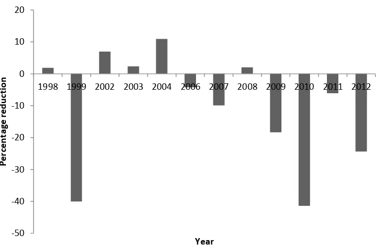
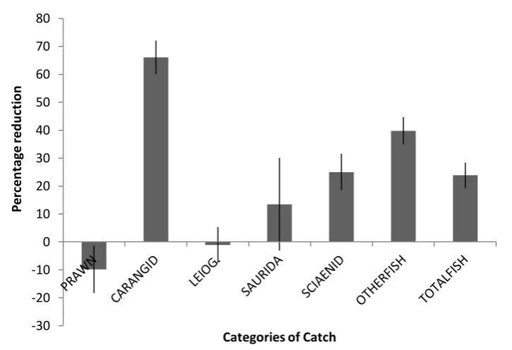
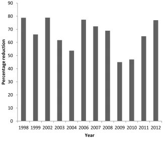
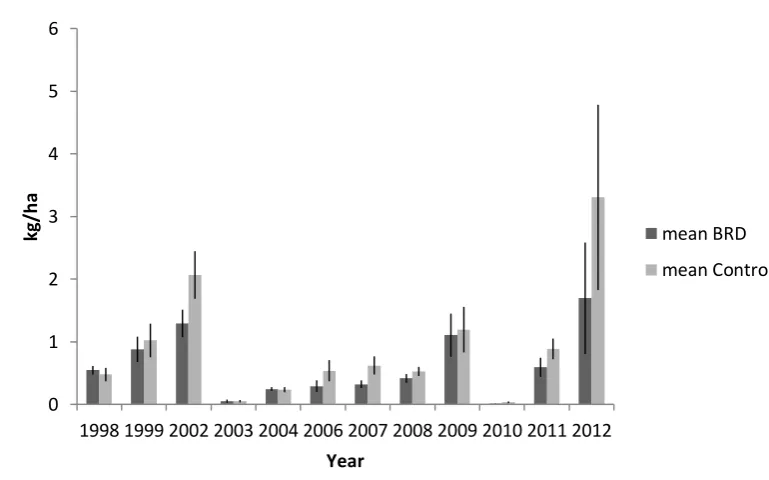
(7) List of Figures Figure 2.1: Location of the study site in Cleveland Bay (19° 10’ S and 146° 50’ E), Townsville, Australia...............................................................................................................13 Figure 2.2: The Jones-Davis By-catch Reduction Device......................................................18 Figure 2.3: Percentage Difference in catch of Prawns for the BRD and Control trawl nets for from 1998- 2012.......................................................................................................................22 Figure 2.4: Mean (+/- SE) catch of Prawns per hectare in the BRD and control net from 1998-2012.................................................................................................................................22 Figure 2.5: Mean (+/- SE) percentage reduction of major categories of catch in the BRD net (relative to the control net) from 1998-2012............................................................................23 Figure 2.6: Percentage Difference of BRD and Control trawl nets for total fish catch from 1998- 2012................................................................................................................................24 Figure 2.7: Mean (+/- SE) Total fish catch per hectare in the BRD and control net from 19982012.........................................................................................................................................24 Figure 2.8: Percentage Difference in catch of Carangidae between the BRD and Control trawl nets from 1998- 2012......................................................................................................25 Figure 2.9: Mean (+/- SE) catch of Carangidae per hectare in the BRD net and the control net from 1998- 2012.......................................................................................................................26 Figure 2.10: Percentage Difference in catch of Sciaenidae for the BRD and Control trawl nets from 1998- 2012...............................................................................................................27 Figure 2.11: Mean (+/- SE) catch of Sciaenidae per hectare in the BRD and control net from 1998- 2012...............................................................................................................................27 Figure 2.12: Percentage Difference in catch of Saurida spp. for the BRD and Control trawl nets from 1998- 2012..............................................................................................................28 Figure 2.13: Mean (+/- SE) catch of Saurida spp. per hectare in the BRD and control nets from 1998-2012......................................................................................................................29 Figure 2.14: Percentage Difference in catch of Leiognathidae for the BRD and Control trawl nets from 1998- 2012.............................................................................................................30. Figure 2.15: Mean (+/- SE) catch of Leiognathidae per hectare in the BRD and the control net from 1998- 2012...............................................................................................................30 Figure 2.16: Percentage Difference in catch “Other fish” for the BRD and Control trawl nets from 1998- 2012.....................................................................................................................31 vi.

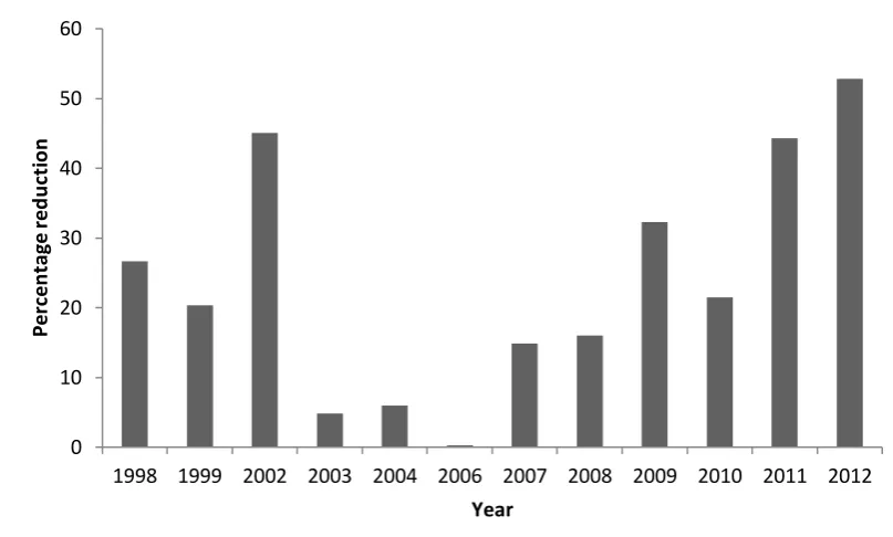
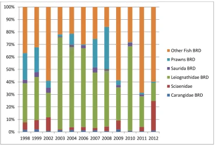
(8) Figure 2.17: Mean (+/- SE) catch of “Other fish” per hectare in the BRD and control net from 1998-2012......................................................................................................................32 Figure 2.18: Catch composition (as % by weight) of the six major groups in the BRD equipped trawl net...................................................................................................................33 Figure 2.19: Catch composition (as %) of the six major groups using the control trawl net............................................................................................................................................33 Figure 3.1: Mean (+/-SE) catch rate (kg/ha) of prawns in the control net from 1998-2012. Years not sampled were 2000, 2001, 2005..............................................................................50 Figure 3.2: Mean (+/- SE) catch rate (kg/ha) of Total Fish in the control net between 1998 and 2012. Years not sampled were 2000, 2001, 2005.............................................................52 Figure 3.3: Mean (+/- SE) catch rate (kg/ha) of Carangidae in the control net from 19982012. Years not sampled were 2000, 2001, 2005....................................................................53 Figure 3.4: Mean (+/- SE) catch rate (kg/ha) of Sciaenidae in the control net from 19982012. Years not sampled were 2000, 2001, 2005....................................................................54 Figure 3.5: Mean (+/- SE) catch rate (kg/ha) of Saurida spp. in the control net from 19982012. Years not sampled were 2000, 2001, 2005....................................................................55 Figure 3.6: Mean (+/- SE) catch rate (kg/ha) of Leiognathidae in the control net from 19982012. Years not sampled were 2000, 2001, 2005....................................................................56 Figure 3.7: Mean (+/- SE) catch rate (kg/ha) of “Other Fish” in the control net from 19982012. Years not sampled were 2000, 2001, 2005....................................................................57 Figure 3.8: Linear Regression of mean catch rate (kg/ha) of Sciaenidae (a), ‘Other Fish’ (b) and ‘Total Fish’(c) in a sampling year against average wet season rainfall two years prior to sampling. The line of best fit explained 28.2% (Sciaenidae); 32% (‘Other Fish’) and 55% (‘Total Fish’) of the variance and was significant (p < 0.05) for all groups...........................59 Figure 3.09: Mean (+/- SE) catch rate (kg/ha) of prawns for all 12 sampling years from 1998-2102 at different phases of the moon. ............................................................................61 Figure 3.10: Mean (+/- SE) catch rate (kg/ha) of Saurida spp. for all 12 sampling years from 1998-2012 at different phases of the moon. ...........................................................................62 Figure 4.1: Ordination of the multispecies fish assemblage in Cleveland Bay from 1998 – 2012. Multi-dimensional Scaling was undertaken using the Bray Curtis similarity index. Different years are colour coded and represented by different symbol types. A symbol type within a year (usually 4 replicates within a year) shows the trawl samples on separate days of sampling. To see which symbols relate to BRD +/- see Figure 4.6.........................................83 Figure 4.2: Ordination of the multispecies fish assemblage in Cleveland Bay from 2010 – 2012. Multi-dimensional Scaling was undertaken using the Bray Curtis similarity index. Different years are colour coded and represented by different symbol types. A symbol type within a year shows the trawl samples on separate days of sampling. To see which symbols relate to BRD +/- see Figure 4.6..............................................................................................84 vii.

(9) Figure 4.3: Ordination of the multispecies fish assemblage in Cleveland Bay from 2006– 2008. Multi-dimensional Scaling was undertaken using the Bray Curtis similarity index. Different years are colour coded and represented by different symbol types. A symbol type within a year shows the trawl samples on separate days of sampling. To see which symbols relate to BRD +/- see Figure 4.6..............................................................................................85 Figure 4.4: Ordination of the multispecies fish assemblage in Cleveland Bay from 2006 – 2009. Multi-dimensional Scaling was undertaken using the Bray Curtis similarity index. Different years are colour coded and represented by different symbol types. A symbol type within a year shows the trawl samples on separate days of sampling. To see which symbols relate to BRD +/- see Figure 4.6..............................................................................................86 Figure 4.5: Ordination of the multispecies fish assemblage in Cleveland Bay from 2006 – 2010. Multi-dimensional Scaling was undertaken using the Bray Curtis similarity index. Different years are colour coded and represented by different symbol types. A symbol type within a year shows the trawl samples on separate days of sampling. To see which symbols relate to BRD +/- see Figure 4.6..............................................................................................87 Figure 4.6: Ordination of the multispecies fish assemblage in Cleveland Bay comparing BRD (+ symbols) and Control (- symbols) net catches. Multi-dimensional Scaling was undertaken using the Bray Curtis similarity index. Different years are colour coded and represented by different symbol types. A symbol type within a year shows the trawl samples with and without a BRD on separate days of sampling...........................................................88. viii.

(10) List of Tables: Table 2.1: Number of trawling days per year, total number of trawls per year and number of replicate groups of trawls per year (number of individual student trips spread over the number of trawling days in a year) from 1998-2012............................................................................16 Table 2.2: Univariate ANOVAs testing effects of BRD and Year of Sampling for all variates and direction of change of variates due to the BRD (as %). The denominator of all F values is 129...........................................................................................................................................23 Table 3.1: Univariate ANOVAs testing the effect of year of sampling on catch rate (kg/ha) for all variates. The denominator of all F values is 244...........................................................51 Table 3.2: Multiple regression results for the effect of 2 year lagged rainfall on catch rate (kg/ha) of all variates. The denominator for all F values is 10................................................51 Table 3.3: Multiple comparison p values (2 tailed) for effects of moon phase on catch rate of prawns, Kruskal-Wallis test: H (3, N=77) p = 0.0015.............................................................60 Table 3.4: Univariate ANOVAs testing for the effect of moon phase on catch rate (kg/ha) for all fish variates. The denominator of all F values is 73. ..........................................................60 Table 4.1: Average dissimilarity (expressed as a percentage) between a specific year and all other years and the number of species accounting for the top 25% of the dissimilarity identified by SIMPER..............................................................................................................82 Table 4.2: Species identified by Simper analysis that accounted for the cumulative top 25% of species differences between the BRD net and the control net. The average dissimilarity between BRD and control nets over the 12 sampling years was 34.42% (this includes all 160 species).....................................................................................................................................89. ix.

(11) List of Appendices: Appendix 1 Table 1.1: Univariate ANOVAs testing the effects of the BRD and Year of Sampling for all variates. The denominator of all F values is 129....................................................................119. Appendix 2 Figure 2.1: Mean (+/- SE) catch rate (kg/ha) of Leiognathidae for all 12 sampling years from 1998-2102 at different phases of the moon. .........................................................................120 Figure 2.2: Mean (+/- SE) catch rate (kg/ha) of Sciaenidae for all 12 sampling years from 1998-2102 at different phases of the moon. .........................................................................120 Figure 2.3: Mean (+/- SE) catch rate (kg/ha) of “Total Fish” for all 12 sampling years from 1998-2102 at different phases of the moon. .........................................................................121 Figure 2.4: Mean (+/- SE) catch rate (kg/ha) of “Other Fish” for all 12 sampling years from 1998-2102 at different phases of the moon. .........................................................................121 Figure 2.5: Mean (+/- SE) catch rate (kg/ha) of Carangidae for all 12 sampling years from 1998-2102 at different phases of the moon............................................................................122 Table 2.1: Multiple regression analysis testing the effect of rainfall on the catch rate (kg/ha) of total fish for all treatments.................................................................................................122 Table 2.2: Multiple regression analysis testing the effect of rainfall on the catch rate (kg/ha) of Carangidae for all treatments............................................................................................122 Table 2.3: Multiple regression analysis testing the effect of rainfall on the catch rate (kg/ha) of Sciaenidae for all treatments..............................................................................................123 Table 2.4: Multiple regression analysis testing the effect of rainfall on the catch rate (kg/ha) of Prawns for all treatments....................................................................................................123 Table 2.5: Multiple regression analysis testing the effect of rainfall on the catch rate (kg/ha) of Leiognathidae for all treatments........................................................................................123 Table 2.6: Multiple regression analysis testing the effect of rainfall on the catch rate (kg/ha) of Saurida spp. for all treatments...........................................................................................123 Table 2.7: Multiple regression analysis testing the effect of rainfall on the catch rate (kg/ha) of ‘Other Fish’ for all treatments............................................................................................123 Table 2.8: Univariate test of significance testing the effect of moon phase on catch rate (kg/ha) for all variates............................................................................................................124 x.

(12) Table 2.9: Univariate test of significance testing the effect of year of sampling on catch rate (kg/ha) for all variates............................................................................................................125 Table 2.10: Tukey’s HSD test comparisons among all years for the Prawn data set...........126 Table 2.11: Tukey’s HSD test comparisons among all years for the “Total Fish” data set...........................................................................................................................................127 Table 2.12: Tukey’s HSD test comparisons among all years for the Carangidae data set...........................................................................................................................................128 Table 2.13: Tukey’s HSD test comparisons among all years for the Leiognathidae data set...........................................................................................................................................129 Table 2.14: Tukey’s HSD test comparisons among all years for the Saurida spp. data set...........................................................................................................................................130 Table 2.15: Tukey’s HSD test comparisons among all years for the Sciaenidae data set...........................................................................................................................................131 Table 2.16: Tukey’s HSD test comparisons among all years for the “Other Fish” data set...........................................................................................................................................132 Appendix 3 Table 3.1: Species identified by Simper as those who cumulatively explained the most 25% dissimilarity in species composition between 1998 and all other years combined. Average dissimilarity between 1998 and all other years was 36.58% (this includes all 160 species)...................................................................................................................................133 Table 3.2: Species identified by Simper as those who cumulatively explained the most 25% dissimilarity in species composition between 1999 and all other years combined. Average dissimilarity between 1999 and all other years was 33.13% (this includes all 160 species)...................................................................................................................................134 Table 3.3: Species identified by Simper as those who cumulatively explained the most 25% dissimilarity in species composition between 2002 and all other years combined. Average dissimilarity between 2002 and all other years was 33.33% (this includes all 160 species)...................................................................................................................................135 Table 3.4: Species identified by Simper as those who cumulatively explained the most 25% dissimilarity in species composition between 2003 and all other years combined. Average dissimilarity between 2003 and all other years was 33.82% (this includes all 160 species)...................................................................................................................................136 Table 3.5: Species identified by Simper as those who cumulatively explained the most 25% dissimilarity in species composition between 2004 and all other years combined. Average dissimilarity between 2004 and all other years was 34.11% (this includes all 160 species)...................................................................................................................................137 xi.

(13) Table 3.6: Species identified by Simper as those who cumulatively explained the most 25% dissimilarity in species composition between 2006 and all other years combined. Average dissimilarity between 2006 and all other years was 35.49% (this includes all 160 species)..................................................................................................................................138 Table 3.7: Species identified by Simper as those who cumulatively explained the most 25% dissimilarity in species composition between 2007 and all other years combined. Average dissimilarity between 2007 and all other years was 34.53% (this includes all 160 species)..................................................................................................................................139 Table 3.8: Species identified by Simper as those who cumulatively explained the most 25% dissimilarity in species composition between 2008 and all other years combined. Average dissimilarity between 2008 and all other years was 37.24% (this includes all 160 species)...................................................................................................................................140 Table 3.9: Species identified by Simper as those who cumulatively explained the most 25% dissimilarity in species composition between 2009 and all other years combined. Average dissimilarity between 2009 and all other years was 33.85% (this includes all 160 species)..................................................................................................................................141 Table 3.10: Species identified by Simper as those who cumulatively explained the most 25% dissimilarity in species composition between 2010 and all other years combined. Average dissimilarity between 2010 and all other years was 36.61% (this includes all 160 species)...................................................................................................................................142 Table 3.11: Species identified by Simper as those who cumulatively explained the most 25% dissimilarity in species composition between 2011 and all other years combined. Average dissimilarity between 2011 and all other years was 34.4% (this includes all 160 species)...................................................................................................................................143 Table 3.12: Species identified by Simper as those who cumulatively explained the most 25% dissimilarity in species composition between 2012 and all other years combined. Average dissimilarity between 2012 and all other years was 35.66% (this includes all 160 species)...................................................................................................................................144 Table 3.13: List of species caught on only one day during the 15 year study period...........144. Appendix 4 Table 4.1: List of species caught in Cleveland bay during the 15 year study period............145 Appendix 5: Table 5.1: Commercial catch data (Grid J21) of Fenneropenaeus merguiensis in March from 1998 – 2011...........................................................................................................................148. xii.

(14) Abstract Fishing gears are often “non-selective”. That is, they frequently catch organisms that are not the target of the fishery. Such organisms are usually referred to as bycatch. Some bycatch can be sold or used, but much of it is often of no value and unwanted. Thus, bycatch is a major problem in fisheries around the world, for both the fishery and the ecosystems from which the bycatch is removed. The prawn trawling industry has in the past captured very high ratios of bycatch to target species, due to the non-selective nature of trawl gear. Fifty to ninety percent of total catch by weight in a prawn trawl net can comprise unwanted species that are mostly discarded. Reducing the amount of unwanted catch in commercial fisheries is of major importance if we are to use fish stocks wisely and conserve global biodiversity. The implementation of bycatch reduction devices (BRDs) has been a major focus of fisheries management over the last two decades. The data for this study were obtained from field sampling in Cleveland Bay, North Queensland, Australia. The sampling was carried out by staff at James Cook University (JCU), assisted by students enrolled in a fisheries science subject at JCU. The equipment, sampling techniques and general area of sampling remained consistent over the entire fifteen year (1998-2012) study period. Prawn trawls were carried out for two or three days in the first two weeks of March for 12 of the 15 years, using the same vessel, the same net configurations, the same trawling procedures, and in the same inshore area of Cleveland Bay. Individual trawl times of 10 minutes duration could be expressed as a swept area of each trawl net of 6000m2, and this also remained consistent over the entire study. For ease of comparison with the broader literature all catch rates are expressed as kg/hectare in this thesis. Thus, it was possible to obtain a long-term, scientific prawn trawling data set in which sampling procedures remained consistent.. xiii.

(15) The first data chapter of this thesis examined the effects of the Jones-Davis BRD on catch rates of prawns and fish bycatch. A total of 244 trawls (each of 10 minutes duration) were carried out in 12 separate years between 1998 and 2012 by the JCU research vessel, James Kirby, rigged as a twin otter trawler. The two prawn trawling nets had different configurations: Turtle excluder device (TED) only (control net); TED and Jones-Davis BRD. The effect of the BRD on catch rates of four major teleost families, all other fish, penaeid prawns, and total fish catch was assessed. The BRD reduced catch rates of total fish bycatch, Carangidae, Sciaenidae and “Other Fish” significantly during the study. A significant year (time) effect on catch rates was detected for all variates investigated, but no significant interaction between the BRD and year of sampling was detected for any variates. Thus, the effect of the BRD was consistent across all years. Prawn retention using this device was high, with no significant difference in prawn catch rates between the two nets The BRD reduced catch rates of total fish (by 23.7%+/- SE 4.91), carangids (trevallies) (by 65.9%+/-SE 3.48) and sciaenids (croakers) (by 24.6% +/-SE 6.82) significantly. The BRD was an effective tool in reducing catch rates of fast, strong swimming semi-pelagic and pelagic fish species, but ineffective in reducing catch rates of slow swimming benthic and demersal fish species (e.g. Leiognathidae, Saurida spp.). Slow swimming benthic species comprise the majority of the tropical inshore fish assemblage. Averaged over the 15 years of the present study, the 23.7 % reduction in total fish catch means that the Jones-Davis BRD was ineffective in eliminating 76.3% of the fish bycatch in this tropical fish assemblage in Cleveland Bay. Attempts to design BRDs specifically for tropical Indo-West Pacific conditions have reduced fish bycatch in prawn trawl nets by 2040%, at best. Thus, this study of the Jones-Davis BRD in Cleveland Bay is consistent with these other studies, even when the BRD was not designed for local conditions. The second data chapter of this thesis investigated the effect of environmental factors on inter-annual xiv.

(16) variations in trawl catch rates in a tropical fish assemblage in Cleveland Bay over 15 years. Environmental factors investigated included rainfall, tidal state and moon phase. Rainfall two years prior to sampling affected total fish catch rates significantly (p< 0.05; R2 adj. = 0.305), again with catch rates enhanced by rainfall. The two year lag effect may be due to a two year lag in recruitment of fish to the fishery. This potential delayed recruitment into the fishery could be explained by migration of sub-adults out of the estuaries and mangrove forests into the near shore habitats where trawling occurred, combined with fish growing to a catchable size. Catch rates of prawns (mostly banana prawns, Fenneropenaeus merguinesis) were not affected by rainfall in this study. Catch rates of prawns and Saurida spp. (Lizardfish) were significantly higher on the full moon (p < 0.05). The effects of environmental drivers like rainfall and moon phase on inter-annual variations in catch rates of both prawns and fish in this tropical fish assemblage could only have been detected by consistent, long-term sampling. The third data chapter of this thesis examined inter-annual variations in the species composition of the tropical fish assemblage in Cleveland Bay from 1998 to 2012. A total of 160 teleost species were recorded in the 244 trawls made over 15 years. A Multi-dimensional scaling (MDS) analysis of the species presence-absence data demonstrated that there was no long-term, systematic shift in the species composition of the tropical fish assemblage in Cleveland Bay over the 15 years of study. That is, there was no evidence that the assemblage structure changed from one state to another, despite inter-annual variations in species composition and environmental conditions. In addition, there was little evidence of differences in species composition of the trawl catch between nets fitted with and without the Jones-Davis BRD. Long term monitoring studies are an important tool in fisheries research. Usually such studies involve collection of catch rate data from commercial fisheries. Gear efficiencies and fishing xv.

(17) effort often vary in long-term studies of commercial fisheries. Long-term scientific, fisheryindependent, surveys using completely consistent methods are rarer, often because funds to support them are limited. The long-term consistency of sampling in this study was critical in revealing inter-annual variations in performance of a BRD, identifying environmental drivers of trawl catch rates, and demonstrating the long-term consistency of species composition of a tropical fish assemblage.. xvi.

(18) Chapter 1 General Introduction:. The role of biodiversity in maintaining ecosystem services for a growing human population is considered important to the food supply of current and future human generations. Local species richness may enhance ecosystem stability and productivity (Loreau et al., 2001; Worm et al., 2006; Worm and Branch, 2012). Such effects are more difficult to demonstrate at a landscape level (Halpern et al., 2009; Kappel et al., 2012a). Management of the world’s ocean resources is a challenge, given the geographically large extent and taxonomically complex nature of these resources (Levin et al., 2009; Worm et al., 2006). Implementing local findings on large spatial scales has proven to be more difficult in marine than in terrestrial ecosystems (Hendriks et al., 2006). The marine environment provides many goods and services, one of the most important being food supply for a growing human population (Holmlund and Hammer, 1999; Peterson and Lubchenco, 1997; Smith et al., 2010). An everincreasing proportion of the human population lives near coasts , and this human population pressure often results in loss of services due to pollution and overfishing (Crain et al., 2009; Kappel et al., 2012b). This can have very clear detrimental effects on marine ecosystems. Overexploitation of marine resources, pollution of the marine environment, and habitat destruction can be directly linked to changes in marine biodiversity (Adger et al., 2005; Dulvy et al., 2006; Worm et al., 2006). Detecting the extinction of marine species is often difficult, but a very convincing literature documenting rapid decline of populations, species diversity, or entire functional groups in the marine environment exists (Pauly and Christensen, 1995; Pauly et al., 2002; Pauly et al., 2000; Pauly et al., 2005; Worm et al., 2006; Worm et al., 2005). It is now widely accepted that since the late 19th century, commercial fisheries have substantially reduced the abundance of target populations and 1.

(19) affected associated fish assemblages (Pauly and Christensen, 1995; Pauly et al., 1998; Pauly et al., 2005; Worm et al., 2006). Fishing affects the life history parameters of both targeted and non-targeted marine species and in some circumstances has resulted in local extinction of certain species (Jennings et al., 2005; Pope et al., 2006; Rogers and Ellis, 2000; Tonks et al., 2008). Approximately 148 million tonnes of fish were supplied to global markets from fisheries and aquaculture in 2010 (FAO, 2012a). Sustained growth in fish production and improved distribution channels have led to a growth in world fish supply in recent decades with an average growth rate of around 3.2% per year (FAO, 2012). Per capita human fish consumption has doubled in the last 40 years with an average of 18.6kg in 2010 (FAO, 2012). While inland fisheries have increased output over the last few years, marine fisheries production has been declining in the last two decades (Pauly et al., 2002; Pauly and Froese, 2012; Watson et al., 2012) even though fishing effort has increased and technological advances and biological knowledge of the target species have been improving (FAO, 2012). Watson et al (2012) recently showed that, on a global scale, marine fishing effort has increased 10-fold in the past 60 years, but catch per unit effort has halved over the same period. Global marine fisheries production in 2010 was estimated to be around 77.4 million tonnes. The proportion of under- exploited fish stocks has decreased gradually since the early 1970’s and currently only around 13% of global fish stocks are not fully exploited, with 57% of stocks being fully exploited and around 30% being over-exploited (FAO, 2012; Froese et al., 2012). The ever increasing demand for fish has been compensated for by rapidly expanding aquaculture production, which has expanded 12-fold in the last three decades, currently producing around 60 million tonnes of fish, molluscs and crustaceans (FAO, 2012). Declining marine catches combined with increasing numbers of overexploited fish stocks clearly shows that the state of the world’s marine fisheries is worsening (FAO, 2012a; Firth 2.

(20) and Hawkins, 2011; Pauly, 2009; Pauly and Froese, 2012; Pauly et al., 2005; Watson et al., 2012). This overexploitation of marine resources causes negative ecological impacts, reduces fisheries production, and results in negative social and economic consequences (Christensen, 2005; FAO, 2012a; Pauly and Froese, 2012; Worm et al., 2006). Overfishing of particular fish species has been seen as the major driver for collapsing fish stocks around the world (Christensen et al., 2003). Originally fish stocks were managed to attain sustainable harvest of the target species (Brewer et al., 2006). More recently there has been a greater interest in managing the whole ecosystem (Christensen and Pauly, 2004; FAO, 2012b; Foley et al., 2010; Levin et al., 2009). This approach does not focus on sustainable harvest of the target species alone, but also on the sustainable management of the associated ecosystem, and the social and economic benefits that can be derived from such approaches (Levin et al., 2009; Worm et al., 2006). In order for such management to be implemented, a thorough understanding of ecosystem processes and dynamics is desirable. Thus, we need to better understand which parts of ecosystems are not only important in social and economic terms, but in a more holistic, ecological context. The growing commitment to an ecosystembased approach to fisheries means that fisheries managers need to take into account the wider environmental impacts of fishing (Thrush and Dayton, 2002; Tillin et al., 2006). Fisheries management must ensure that fishing effects are sustainable not only in terms of the target species but in terms of ecosystem maintenance (Pikitch et al., 2004; Pope et al., 2006). Alterations in species composition of marine ecosystems may alter the functional diversity of communities and lead to modifications of ecosystem function (Solan et al., 2004; Tillin et al., 2006). A major problem of many fisheries is the disturbance and alteration of habitat associated with the fishery (Dayton et al., 1995; Olsgard et al., 2008; Thrush and Dayton, 2002). This is particularly important for fisheries that target species that are closely associated with the 3.

(21) benthic environment (Thrush et al., 1998; Thrush and Dayton, 2002). Demersal trawling can have major habitat modification effects, and can be non-selective in terms of catch composition at times(Christensen, 2005; Dayton et al., 1995; Olsgard et al., 2008; Schratzberger et al., 2002; Schratzberger and Jennings, 2002; Tillin et al., 2006). Demersal bottom trawls can remove a large proportion of the benthic flora and fauna in trawled areas (Auster and Langton, 1999; Auster et al., 1996; Olsgard et al., 2008; Sainsbury, 1998; Wells, 2007). Long-term trawling on the North West shelf of Australia was shown to remove up to 90% of large sponges (Sainsbury, 1998; Sainsbury et al., 1993). This removal of epibenthos also affects the associated fish community and Sainsbury et al. (1997) reported that over 20 years the catch rate of large sponges in trawls on the North West Shelf of Australia fell nearly 400 fold. This drop in catch rate of sponges was associated with a 4-5 fold decrease in catch rates of reef fish such as lutjanids and lethrinids (Burridge et al., 2006). Studies have shown that a single prawn trawl in the Australian Northern Prawn Fishery can remove around 520% of most classes of epibenthos (Burridge et al., 2003). Cumulative trawling over many years could clearly have dramatic impacts on entire ecosystems (Auster and Langton, 1999; Pitcher et al., 2000). While marine benthic communities on soft substrata are capable of coping with intermittent disturbances such as severe storms, they are less likely to recover from chronic long- term disturbance caused by bottom trawling (Burridge et al., 2006; McConnaughey et al., 2000; Tillin et al., 2006).. Demersal trawling, particularly trawling that targets prawns in tropical regions, can be a nonselective form of fishing (FAO, 2012). The potential impacts of discarding extremely high amounts of unwanted non-target organisms has been the focus of major political, scientific and conservation debates over the last 30 years (Alverson et al., 1994; Andrew and Pepperell, 1992; Brewer et al., 1998; Brewer et al., 2008; Broadhurst et al., 2012b; Broadhurst et al.,. 4.

(22) 2008; Kelleher, 2009; Poiner et al., 1998; Robins et al., 1999; Robins and McGilvray, 1999; Rochet et al., 2011). While many trawl fisheries may capture large quantities of unwanted species, none are as non-selective as certain demersal finfish and prawn trawls, which account for up to 50% of world fisheries discards (Alverson, 1997; FAO, 2012a; Kelleher, 2009).. Prawns not only provide a valuable source of income to countries and communities but are also a valuable source of protein (FAO, 2012). Prawn production (both wild caught and farmed) was valued at $324.1 million to the Australian economy in 2009- 2010 (Beare et al., 2010).The shrimp and prawn industries continue to be the largest single marine fisheries trade commodity in value terms, accounting for around 15% of the total value of internationally traded fishery products in 2010 (FAO, 2012).. Unfortunately, the tropical prawn trawl fisheries are also the single most non-selective fisheries worldwide in terms of catching large quantities of non-target organisms and discarding them, mostly dead, back into the oceans (FAO, 2012). Typically the ratio of nontarget to target catch rates is between 5:1 and 10:1, and tropical prawn trawling accounts for 27% off all global marine fishery discards by weight. In contrast, prawn trawling accounts for around 2% of global marine fishery production in terms of weight (FAO, 2012).. Non-target organisms captured during commercial fishing are collectively termed bycatch (Andrew and Pepperell, 1992). Bycatch is defined as the indiscriminate capture of all nontarget organisms and non-living materials (debris) while fishing (Earys, 2007). Discards are the unusable or unwanted part of the bycatch that is subsequently thrown back into the sea often dead or dying (Davies et al., 2009). One of the most significant conservation issues in. 5.

(23) fisheries is the effect of removal of bycatch on marine communities and ecosystems (Davies et al., 2009). Estimating the quantity of global fisheries bycatch is often difficult and controversial (Alverson et al., 1994; Alverson, 1997; Davies et al., 2009; Kelleher 2009). Defining exactly what is bycatch can be difficult when there are ambiguities in what is target and what is not in many trawl fisheries (Davies et al., 2009). Even though traditionally all catch other than prawns has been described as bycatch, socio-economic factors, coupled with overfished marine stocks, particularly in developing countries, have led to a very broad usage of the term bycatch in many fisheries (Davies et al., 2009; FAO, 2012). A lack of, or inconsistent, documentation of removal of fish biomass around the world’s fisheries (Froese et al., 2012; Zeller et al., 2007; Zeller et al., 2006; Zeller et al., 2005) makes it difficult to fully understand the extent of the impact that bycatch removal has on the environment and associated ecosystems. Davies et al., (2009) has put forward a new definition of bycatch and defines it as the catch that is either unused or unmanaged.. Discards, especially in the tropical prawn trawling industry, often suffer very high mortality rates (Hill and Wassenberg, 2000). Some of the bycatch species encountered during prawn trawling operations are threatened or endangered species such as turtles, certain shark species, dugongs, sea snakes, sea horses, corals and some fish species (Earys, 2007). Hill and Wassenberg (2000) showed that in the Northern Prawn Fishery only 12% of total discards might survive. Their study also estimated that only around 2% of teleost fish survive after being discarded after trawling and that their chance of being eaten by marine predators was increased. Reduction of unwanted catch and the increased utilisation of bycatch have led to a significant decrease in discards over the last decade around the world (FAO, 2012; Zeller et al., 2005). This can mainly be attributed to the use of more selective fishing gears (especially BRDs), introduction of bycatch and discard regulations, and the improved enforcement of. 6.

(24) regulatory measures (Brewer et al., 2008; Broadhurst et al., 2008; FAO, 2012a; Isaksen et al., 1992; Ocean-Watch, 2004).. In the last 20 years much of the focus of the bycatch problem has been on trying to minimize catch rates of non-target species inside trawl nets, by modifying the fishing gear and thus using more selective fishing methods. The most common modifications are TEDs that aim to eliminate the catch of marine megafauna (e.g. turtles, sharks, rays etc.) and BRDs that aim to reduce the catch of non-target teleost fish (Earys, 2007). While many scientific studies have investigated the effectiveness of different BRDs around the world, (Andrew and Pepperell, 1992; Brewer et al., 1998; Broadhurst et al., 2012b; Broadhurst et al., 2008; Glass, 2000; Robins-Troeger, 1994; Robins-Troeger et al., 1995; Robins and McGilvray, 1999) to date there have been no fishery-independent studies of the effectiveness of BRDs over the long term.. This thesis explores a long-term (1998-2012), fishery-independent, trawl sampling data set that used consistent methods over a 15 year period in a tropical bay in northern Australia. The aims of this thesis are:. 1. To quantify inter-annual variations in the performance of a BRD in a tropical bay where prawns are the target of the fishery and all teleost fish are considered bycatch. 2. To identify what environmental factors (e.g. rainfall, moon phase) may affect the trawl catch rates of both prawns and fish over a 15 year period of sampling. 3. To examine inter-annual variations in the species composition of the tropical fish assemblage and investigate if the BRD affects the species composition of the trawl fish catch.. 7.

(25) Chapter 2 The effectiveness of the Jones-Davis bycatch reduction device (BRD) in a tropical fish assemblage, in Cleveland Bay, Townsville, Australia.. Introduction Until recently the primary aim of management of harvest fisheries was to maximise sustainable yield of the target species (Brewer et al., 2006). The capture of non-target organisms by fishing gears has become a global issue in the past few decades, from the points of view of both sustainability of fisheries and conservation of marine ecosystems (Macbeth et al., 2005b). Prawn trawling fisheries not only capture marine megafauna of conservation interest (e.g. turtles, sharks, rays) but also have the highest ratio of bycatch to target species of any fishery (Alverson, 1997; Alverson et al., 1994; Courtney et al., 2006; Eayrs, 2007). Trawling can account for more than one-third of total global bycatch and discards (Courtney et al., 2006; Davies et al., 2009; Pascoe, 1997). The weight of the bycatch in many tropical trawl fisheries usually exceeds the weight of the target species (penaeid prawns) and can encompass hundreds of different species, mostly teleosts fish (Courtney et al., 2006; Gray et al., 1990; Kennelly et al., 1998; Steele et al., 2002; Stobutzki et al., 2001; Van der Geest, 2000; Watson et al., 1990; Ye et al., 2000). One of the most successful techniques to minimize bycatch of harvest fisheries is to improve the selectivity of fishing gear (Brewer et al., 1997; Macbeth et al., 2005a). BRDs and TEDs are used in modern fisheries in order to reduce the catch of non target species (Brewer et al., 2006; Courtney et al., 2006; Hall and Mainprize, 2005a; Isaksen et al.,. 8.

(26) 1992). Originally BRDs were designed to exclude the catch of marine turtles (Tillman, 1992). Later BRD technology focused on excluding larger fish and elasmobranches, and more recently technological improvements have aimed at excluding smaller bycatch taxa such as small finfish, while retaining target species catch (Broadhurst et al., 2004; Macbeth et al., 2005b; Mitchell et al., 1995; Pichot et al., 2009; Richards and Hendrickson, 2006; Rogers et al., 1997). In recent years much of the research on BRDs has focused on their physical design and upon behavioural factors of target and non-target species that affect the performance of BRDs (Fennessy and Isaksen, 2007; Gabr et al., 2007a, b; Graham et al., 2004; Kim and Whang, 2010; Macbeth et al., 2007; Pichot et al., 2009). BRDs that separate species by their behaviour in the net operate on the principle that fish, unlike weakly swimming invertebrates, have certain characteristic responses to towed trawls (Broadhurst, 2000). Depending on their swimming capability, fish will either avoid trawling gear all together or will be herded within the net (Wardle, 1993, 1983; Wardle and Bailey, 1987; Wardle et al., 1995). Depending on their swimming abilities, fish will eventually tire and fall back towards the cod-end (Broadhurst, 2000). The development of BRDs has focused on this herding effect in terms of choosing an appropriate place for fish escapement from the net (Broadhurst, 2000; Chapman, 1964; Wardle, 1993, 1989). Prawns on the other hand have limited responses to towed trawls. They are not capable of maintaining avoidance responses for more than a short period of time and are quickly forced against the meshes and towards the cod end (Broadhurst, 2000). Much research has focused on altering water flow in parts of the cod end to facilitate fish escapement (Broadhurst et al., 2012a; Broadhurst et al., 2002; Engaas et al., 1999; O'Neill et al., 2005). BRDs are often placed in areas of reduced water flow, where fish have the chance to escape through openings in the net. This is particularly important in prawn fisheries that occur in turbid water, as visual stimuli might be less important in inducing behavioural 9.

(27) escape responses (Engaas et al., 1999). Reduced water flow is not only important in inducing behavioural escape responses but also in allowing an increased number of fish to be physiologically able to escape (Broadhurst, 2000; Broadhurst et al., 2002; Wardle, 1993, 1983, 1989). Differences in body shape, swimming ability, and myotomal muscle distribution all play important roles in the ability of fish species to escape the trawl net through a BRD (Sfakiotakis et al., 1999; Videler, 1993; Wardle and Bailey, 1987; Wardle et al., 1995). Most pelagic and semi-pelagic fish have a high percentage of red muscle fibres, a carangiform or sub-carangiform swimming mode and a very streamlined body permitting endurance swimming at high speeds (Sfakiotakis et al., 1999; Wardle et al., 1995). Red muscle fibres are aerobic and allow fish to maintain high cruising speeds for prolonged periods (Wardle et al., 1995). Benthic and bentho-pelagic species have myotomes dominated by white muscle fibres which use anaerobic phosphorylation and produce lactic acid as a byproduct (Videler, 1993). This build up of lactic acid reduces muscle contraction capacity and is characteristic of fish with weak sustained swimming ability (Videler, 1993). No single BRD is effective in reducing the catch of all teleost bycatch species found in all fisheries (Gorman, 1997). The design and deployment of BRDs has to be matched to the particular fish assemblage and environmental conditions encountered in the fishery (Broadhurst et al., 2012b). Hence, most BRDs were designed for a particular fishery and often designs are altered when used in another part of the world (Broadhurst, 2000). Brewer at al. (1998) tested sixteen different BRD designs in a Northern Prawn Fishery. Each design provided a degree of bycatch reduction and prawn retention, but the performance of different designs was strongly affected by weather and fishing procedures (Brewer et al., 1997; Broadhurst, 2000). However, some BRDs specifically a combination of the fish eye (Broadhurst, 2000; Rogers et al., 1997; Watson and Taylor, 1996) and Nordmore grid (Broadhurst and Kennelly, 1996; Broadhurst et al., 1996; Richards and Hendrickson, 2006) 10.

(28) were effective in consistently reducing fish bycatch by 25% with minimal loss of prawns (Brewer et al., 1998). The fish eye BRD was also reported to be effective in the Caribbean Shrimp Fishery with bycatch reduction rates of 30.7% (Balmori-Ramírez et al., 2003). Bycatch weight reduction of 32% was reported in the New South Wales prawn fishery using the Morrison Soft TED (Andrew et al., 1993), and Robins-Troeger (1994) found that the same device reduced bycatch by 29% in Morten Bay, Queensland. The Jones-Davis BRD has a hard TED (aluminium grid) to exclude large bodied bycatch (turtles, sharks, rays) and then uses a radial escape section and a fish scarer to initiate escape behaviour of strong-swimming teleost bycatch (Broadhurst et al., 2012a; Rogers et al., 1997; Watson et al., 1999). The radial escape section was originally based on a BRD component called a “finfish separator” (Watson et al., 1990). The performances of various designs of the radial escape section have varied significantly, with reductions in fish bycatch of between 2040% by weight (Broadhurst et al., 2012a). The Jones-Davis device has had different levels of success in different places. Watson and Foster (1997) reported a 58% reduction in teleost bycatch when trawl nets were equipped with the Jones-Davis BRD in the Gulf of Mexico. Van der Geest (2000) reported a 19% reduction in teleost bycatch in Cleveland Bay northern Australia. Reductions in teleost bycatch of 43.9% and 33.5% using two modifications of the Jones-Davis BRD (a Double hoop Jones-Davis; a Modified Jones-Davis) were reported in the Gulf of Mexico and in the Caribbean of Colombia (Foster and Scott-Denton, 2004; Manjarres et al., 2008). The testing of BRDs in different environments and under different conditions is important for the future development and optimization of these devices, so that optimal designs are used in each fishery (Salini et al., 2000). Environmental and physical aspects of the fishery, and physiological and behavioural aspects of the fish are important considerations for choosing the most effective BRD for a particular fishery. Efficient functioning of BRDs will reduce 11.

(29) bycatch, reduce fishing costs and duration of fishing and help minimize trawling impacts on the environment (Brewer et al., 1996; Foster and Vincent, 2010). The aim of this chapter was to investigate the effectiveness of the Jones-Davis BRD in the Cleveland Bay prawn trawl fishery, northern Australia. Data from 12separate years of trawling over a 15 year period (1998-2012) with a BRD net and a control net will be analysed to examine the inter-annual variations in efficiency of the BRD.. 12.

(30) Materials and Methods: Site Description: Cleveland Bay , located at 19° 10’ S and 146° 50’ E (Figure 2.1), is approximately 17km long, 25km wide and covers an area of approximately 300km2 (Cruz-Motta and Collins, 2004; Sinclair, 1991). The bay is shallow with an average slope of 0.7m/km dropping to only 15m depth at its outermost limit (Hardy, 1991).Cleveland Bay is enclosed by Cape Cleveland to the southeast, the mainland to the southwest and Magnetic Island to the northwest. The bay is open to the north east and is the harbour for north Queensland’s largest city, Townsville (Reichelt and Jones, 1994). The city has an important port industry where large volumes of mineral goods and other resources are transported. Access to the port is via a 13km long dredged sea channel maintained to a depth of approximately 11m, known as the Platypus channel (Hardy, 1991; Sinclair, 1997).. Figure 2.1: Location of the study site in Cleveland Bay (19° 10’ S and 146° 50’ E), Townsville, Australia. 13.

(31) Cleveland Bay sediment is affected by terrigenous material contained in runoff from two major river systems, the Burdekin River and the Ross River (Carter et al., 1993; Orpin et al., 2004; Wolanski and Jones, 1981). The mean annual rainfall in Townsville is 1146mm (Australian Bureau of Meteorology). An average 80% of the annual precipitation occurs during the months from December to March (Walker, 1981b). Rivers and creeks rise and fall rapidly in response to heavy rains in the wet season, while during the dry winter many creeks cease to flow all-together (Walker, 1981a; Wolanski and Jones, 1981). Cleveland Bay receives direct runoff from the Ross River with a catchment area of 998km2 and an approximate average annual water discharge of 0.49 x 109m3 and from Alligator Creek which has a catchment of 265km2 (Lambrechts et al., 2010; Walker, 1981b). The Burdekin River, the second largest river system in Australia, is located 80 km south east of Cleveland Bay with an approximate average annual discharge of 9.8 x 10 9m3 (Walker, 1981b). The Burdekin River has been found to be an important contributor of fine sediment to Cleveland Bay (Furnas, 2003). During the wet season, increased river discharge lowers coastal salinity levels, increases dissolved nutrient concentrations and increases suspended sediment loads, leading to an increase in turbidity levels (Carter et al., 1993; Orpin et al., 2004; Wolanski and Jones, 1981). During the dry season from around May to October rainfall and river discharge are minimal while water temperatures remain relatively high leading to an increase in evaporation and elevated salinity levels (Walker, 1981a; Walker, 1981b; Wolanski and Jones, 1981). The substratum composition is relatively homogenous throughout Cleveland Bay, consisting of mud and sandy mud (Carter et al., 1993). Bottom mud is stable, being resuspended only under rare strong swell and storm events. However its distribution has been greatly influenced by the dumping of dredged materials from Townsville harbour since the late 70’s (Jing and Ridd, 1997; Lambrechts et al., 2010; Wolanski et al., 1992). There is a net transport 14.

(32) of fine sediment from the dredged material dump site at the outer north-east part of the bay to the more inshore waters leading to an increase of suspended solids and turbidity (Wolanski and Gibbs, 1992; Wolanski et al., 1992). The epibenthic community in Cleveland Bay is relatively homogeneous and has been reported to be resilient to disturbances such as dredged material disposal (Cruz-Motta and Collins, 2004; Sondita, 1997; Watson et al., 1990). The soft bottom benthic macrofaunal community has been reported to be homogenous with slight variations in fish assemblage structures possibly related to depth (Van der Geest, 2000). The demersal community is diverse with 175 fish species recorded in the bay, with the fish assemblage dominated by Leiognathidae (Cabanban, 1991; Sondita, 1997;Van der Geest, 2000). The bay is also an important shark nursery for at least eight different species from two different families (Carcharhinidae and Sphyrnidae) (Simpfendorfer and Milward, 1993).. Sampling Design:. The study had two factors: Presence/ Absence of a Jones-Davis BRD, and time (Year of sampling). The first treatment involved fitting one of two trawl nets on the pair trawler James Kirby with a Jones-Davis by-catch reduction device. The other net was a control net. Both nets were standard nets used in the commercial tropical prawn trawling fishery around northern Australia. Mesh size was 4.5cm from knot to knot. Wooden otter boards 1.5m by 1m were used to open the trawl net laterally, the top of the mouth of the net had 3 floats, and the bottom of the mouth of the net had a tickler chain. Mesh size of the codend was 4.5cm and codend length was 100 meshes. Both trawl nets (BRD+ and BRD-) were set up in twin configuration and sampled at the same time, the net fitted with the BRD was sampling on the 15.

(33) port side and the control net was positioned on the starboard side of the vessel. The same nets and BRD were used for the entire study but repairs were made whenever deemed necessary. During trawling, nets were sampling at a distance of 15-25m apart from each other. Port and starboard biases were assumed to be insignificant in the current study and nets were assumed to be sampling the same population of fish independently of one another as the scale of schooling demersal fish is usually less than this distance (Van der Geest, 2000). The second treatment, time, involved sampling for 2-3 days in the first week of March for 12 of 15 consecutive years, from 1998 – 2012. In three of these years (2000, 2001 and 2005) sampling was not carried out due to technical problems or unavailability of the vessel. Therefore, data of only 12 years will be analysed here. All trawling occurred during daylight between 8:00am and 4:30pm. The number of days trawled each year, the number of trawls per year and the number of replicate groups of trawls in a year are listed in Table 2.1. Trawls were conducted in front of the mouth of Ross River between 19° 13’ to 19° 16’S and 146° 49’ to 146° 53’E at depth of 2.5-6.5m (Figure 2.1).. Year. Days Trawled. Total Number of trawls. Number of replicate groups of trawls. 1998 2 16 4 1999 2 16 8 2002 2 20 6 2003 2 20 6 2004 2 16 5 2006 3 27 9 2007 2 24 7 2008 2 21 7 2009 2 24 6 2010 2 24 6 2011 2 20 6 2012 2 24 7 Table 2.1: Number of trawling days per year, total number of trawls per year and number of replicate groups of trawls per year (number of individual student trips spread over the number of trawling days in a year) from 1998-2012. 16.

(34) Field work was conducted from the RV James Kirby research vessel. The James Kirby is a modified twin otter trawler, 19.5m long and 5.2m wide. Trawl nets used during sampling were standard nets used in the commercial prawn fishery and had a 4.5cm diamond mesh. Trawls were conducted at haphazardly chosen locations just outside the mouth of Ross Creek. Each trawl lasted for ten minutes at a constant speed of 4.2 km/hour, with each net sweeping an area of 6000m2 during this time unit (Cabanban, 1991; Van der Geest, 2000). Catch rates will be expressed as kg/ha in the remainder of the thesis. The trawl duration of ten minutes was chosen as it allowed for a greater number of replicate trawls to be completed in one day and has been shown to be sufficient to sample a representative component of the fish assemblage of the Cleveland Bay (Cabanban, 1991; Van der Geest, 2000). Scientific short term trawls have been shown to be representative in terms of sampling size structure and species composition of commercial long term trawls (Hannah and Jones, 2007; Wassenberg et al., 1998). However, it is acknowledged that short duration trawls may under sample some species of larger, faster swimming species of teleost fish.. After each trawl, catch was sorted on deck by students and Prof. Garry Russ. Catch was sorted into six different categories: Prawns (Fenneropenaeus merguiensis); Carangidae; Leiognathidae; Saurida spp.; Sciaenidae and other fish (the latter category consisted of all other species of fish not included in the four fish categories listed). On trawls which landed a very high biomass, sub-samples were taken, and the total weight of different categories in the trawl was estimated by multiplying up to account for sub-sampling. Once the catch was sorted, wet weight biomass (to +/- 0.05kg) of each category was measured using butchers hook scales. Replicate trawl samples, once sorted and weighed, were then frozen for laboratory analysis.. 17.

(35) The Jones-Davis By-Catch Reduction Device. The Jones-Davis BRD was designed in the South-eastern United States by Leroy Jones and Harry Davis. The device has both active and passive components that aim to reduce the catch of non-target species (Figure 2.2). The passive BRD is the TED. The TED uses a physical sorting method to release larger species of bycatch such as sharks, rays and turtles from the net. It consists of an aluminium grid that is placed approximately two thirds of the way into the trawl net and sits at an angle of approximately 45°. An escape opening is placed at the base of the grid allowing the bigger organisms to escape while target species are retained in the net.. Figure 2.2: The Jones-Davis Bycatch Reduction Device.. The active component of the Jones-Davis BRD is designed to minimize the bycatch of smaller species, such as fish. It was originally designed to minimize capture of juvenile red snapper (Lutjanus campechanus) and mackerel in the South-eastern United States (Foster, 1999; Nance and Scott-Denton, 1997; Watson et al., 1999). The device aimed at utilizing the superior swimming capability of red snapper and other demersal fish species, compared to prawns, to enhance escapement from the trawl nets (Watson et al., 1999). It was designed to. 18.

(36) actively scare the fish and use their natural predatory avoidance response to escape the net, and also to create pockets of reduced water flow velocity to facilitate this escapement (Foster, 1999). Three main components of the Jones-Davis BRD were used to achieve this. Firstly an accelerator funnel, which concentrates the catch into a smaller area just forward of the fish stimulator (Figure 2.2). The funnel opens onto the fish stimulator which provides a visual and physical stimulus to trigger a predatory avoidance response that overrides the optomotor response (stabilization during free locomotion through an involuntary displacement from a straight course) exhibited by some fish species (Arnold, 1974; Van der Geest, 2000; Wastson and Foster, 1997). The trawl net surrounding the funnel has escape openings placed longitudinally along the trawl net, that allow strong swimming fish to swim forward against the direction of water flow, around the accelerator funnel, and either up or down to exit the net via the escape openings (Figure 2.2). In contrast to some other BRD designs, the escape openings used in the Jones-Davis BRD have no mesh on them which reduces injury to the escaping fish (Gabr et al., 2007a; Van der Geest, 2000).. Laboratory Analysis:. All prawn and fish bycatch were identified to at least the level of genus, and usually to species, in the laboratory.. Effectiveness of the Jones-Davis BRD. The effectiveness of the Jones-Davis BRD was tested using a factorial ANOVA with year and presence/absence of the BRD as the fixed two factors and total wet weight biomass (kg/ha) the dependant variable. This enabled the testing of year and BRD effects on biomass, and interaction between these two factors. Statistical tests were conducted at 95% confidence. 19.

No results found