Time-Varying Optimization and Its Application to Power System Operation

(1)

Power System Operation

Thesis by

Yujie Tang

In Partial Fulfillment of the Requirements for the Degree of

Doctor of Philosophy

CALIFORNIA INSTITUTE OF TECHNOLOGY Pasadena, California

2019

(2)

(3)

ACKNOWLEDGEMENTS

My years at Caltech have truly been a precious experience and have shaped my research style. Foremost, I would like to express my sincere gratitude to my advisor, Professor Steven Low, for his generous support and invaluable guidance through my studies and research. Steven has always inspired me by his passion, intelligence, pa-tience, and hardworking attitude. His philosophy of research has greatly influenced my thoughts and is something I will always admire and try to emulate in my future career.

I would also like to thank Professor Adam Wierman, Professor Venkat Chan-drasekaran, and Professor Babak Hassibi for being my thesis committee members and providing brilliant comments and suggestions.

My sincere thanks also go to Professor Emiliano Dall’Anese at University of Col-orado Boulder and Andrey Bernstein at National Renewable Energy Laboratory for their strong support of my research. It has always been a great pleasure to work with them.

I greatly appreciate the support from current and previous members of Netlab. My early years at Caltech would not have been smooth without the help from Lingwen Gan, Changhong Zhao, Qiuyu Peng, and Niangjun Chen. Discussions with Daniel Guo and John Pang have always been enlightening and valuable. It is also pleasing to see younger generations of Netlab making great contributions to state-of-the-art research, stimulating me to gain more confidence and diligence.

(4)

ABSTRACT

The main topic of this thesis is time-varying optimization, which studies algorithms that can track optimal trajectories of optimization problems that evolve with time. A typical time-varying optimization algorithm is implemented in a running fashion in the sense that the underlying optimization problem is updated during the iterations of the algorithm, and is especially suitable for optimizing large-scale fast varying systems. Motivated by applications in power system operation, we propose and analyze first-order and second-order running algorithms for time-varying nonconvex optimization problems.

The first-order algorithm we propose is the regularized proximal primal-dual gradi-ent algorithm, and we develop a comprehensive theory on its tracking performance. Specifically, we provide analytical results in terms of tracking a KKT point, and derive bounds for the tracking error defined as the distance between the algorithmic iterates and a KKT trajectory. We then provide sufficient conditions under which there exists a set of algorithmic parameters that guarantee that the tracking error bound holds. Qualitatively, the sufficient conditions for the existence of feasible parameters suggest that the problem should be “sufficiently convex” around a KKT trajectory to overcome the nonlinearity of the nonconvex constraints. The study of feasible algorithmic parameters motivates us to analyze the continuous-time limit of the discrete-time algorithm, which we formulate as a system of differential inclu-sions; results on its tracking performance as well as feasible and optimal algorithmic parameters are also derived. Finally, we derive conditions under which the KKT points for a given time instant will always be isolated so that bifurcations or merging of KKT trajectories do not happen.

(5)

be viewed as an extension of the sequential quadratic program in the time-varying setting.

(6)

PUBLISHED CONTENT AND CONTRIBUTIONS

[1] Y. Tang, E. Dall’Anese, A. Berstein, and S. Low. Running primal-dual gradient method for time-varying nonconvex problems, 2018, arXiv:1812.00613. URL https://arxiv.org/abs/1812.00613.

Y. Tang participated in formulating the problem and proposing the algorithm, derived the theorerical results, prepared the simulation, and participated in the writing of the manuscript.

[2] Y. Tang, E. Dall’Anese, A. Berstein, and S. H. Low. A feedback-based regularized primal-dual gradient method for time-varying nonconvex opti-mization. In Proceedings of the 57th IEEE Conference on Decision and Control (CDC), pages 3244–3250, Miami Beach, FL, USA, Dec. 2018. doi:10.1109/CDC.2018.8619225.

Y. Tang participated in formulating the problem, proposing the algorithm, and deriving the theoretical results, prepared the simulation, and participated in the writing of the manuscript.

[3] Y. Tang, K. Dvijotham, and S. Low. Real-time optimal power flow. IEEE Transactions on Smart Grid, 8(6):2963–2973, 2017. doi:10.1109/TSG.2017.2704922.

Y. Tang participated in formulating the problem, proposed and analyzed the algo-rithm, prepared the simulation, and participated in the writing of the manuscript. [4] Y. Tang and S. Low. Distributed algorithm for time-varying optimal power flow. In Proceedings of the 56th IEEE Conference on Decision and Control (CDC), pages 3264–3270, Melbourne, VIC, Australia, Dec. 2017. doi:10.1109/CDC.2017.8264138.

(7)

LIST OF ILLUSTRATIONS

Number Page

1.1 The distances to the optimal trajectory kxb(t) − x∗(t)k and kxr(t) − x∗(t)k, and the objective value differencesc(xb(t),t) −c(x∗(t),t)and

c(xr(t),t) −c(x∗(t),t)of the two optimization schemes. . . 6 2.1 Illustration of condition (2.25). This condition is essentially on: (i)

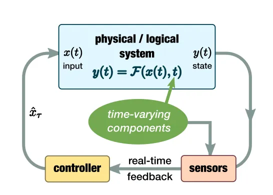
time-variability of a KKT point, (ii) extent of the contraction, and (iii) maximum error in each iteration. Note that in the error-less static case (i.e.,ση =e= 0), this condition is trivially satisfied. . . 31 4.1 Diagram of the control of a time-varying system. The system’s

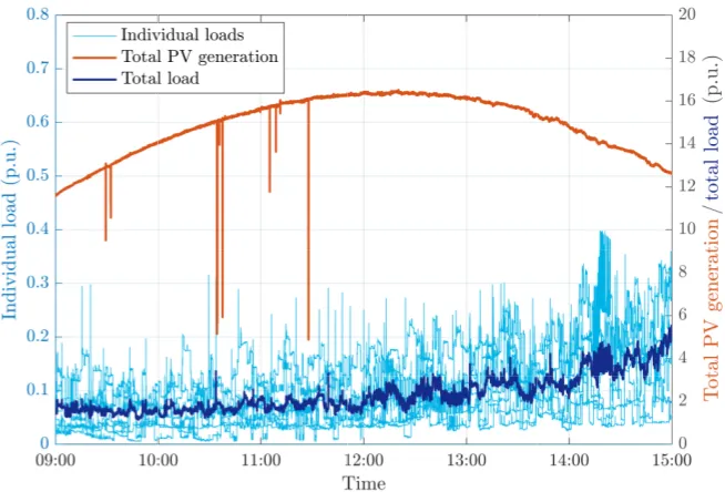
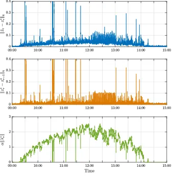
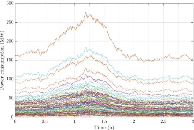
input-state relation is given byF, which is influenced by some time-varying components. . . 116 4.2 Topology of the distribution test feeder. . . 127 4.3 Profiles of individual loads pL_τ,i,i ∈ N, total loadÍ

i∈N pL_τ,i and total photovoltaic (PV) generationÍ

i∈NPVp

PV

τ,i. . . 128 4.4 Illustrations ofzˆτ −z∗_τ

_η,

z_τ∗−z∗_τ−

1

_ηandα λ_τ∗

. . . 129

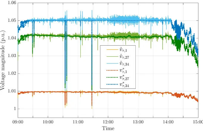
4.5 The voltage profiles ˆvτ,iandv∗_τ,ifori =1, 27 and 34. . . 130 4.6 Load profiles used for simulation. . . 143 4.7 Illustrations ofkxˆτ−x∗,τpk, kx∗,τp−x_τ−∗,p₁k,(Fτ(xτ∗,p) −Fτ(xˆτ))/F_τ(xτ∗,p)

andF_τ(x∗,τp). . . 144 4.8 Voltage profiles of the buses whose voltages have ever violated the

(9)

LIST OF TABLES

Number Page

3.1 Averaged tracking errors of the first-order method and the second-order method applied to the problem (3.34). . . 102 4.1 The locations and normalized areas of the PV panels, and the rated

(10)

C h a p t e r 1

INTRODUCTION

1.1 Overview of Time-Varying Optimization

Suppose we are given a physical or logical system, and for each time t ∈ [0,T], the optimal operation of the system can be modeled as the following optimization problem:

min

x c(x,t)

s.t. f(x,t) ≤ 0.

(1.1) Here x ∈ _Rn is the decision variable that will be applied for operating the system,

c(x,t)is the objective function, and f(x,t)gives the constraints at timet. It can be seen that (1.1) gives an optimization problem that evolves with time. We focus on the situations where the maps x 7→ c(x,t) and x 7→ f(x,t) will only be revealed at timet and their prior predictions are not available. This is a typical setting of a time-varying optimization problem.

In most situations where digital computers are used to solve this problem, we discretize the period[0,T]by a sequence(tτ)_τK₌₁satisfying 0 < t1 < . . . < tK ≤ T, and obtain the following sequence of sampled problems:

min

x cτ(x) s.t. fτ(x) ≤0,

(1.2)

where τ ∈ {1, . . . ,K} labels the discrete time index, and cτ and fτ denote the sampled versionsc(·,tτ)and f(·,tτ). Traditionally, each instance of (1.2) is solved in thebatchscheme abstracted as follows:

For eachτ= 1,2, . . . ,K,

1. Collect problem dataD(tτ)att =tτ, and construct the initial iteratez_τ0. 2. Repeat

z_τk =T z_τk−1;D(tτ) (1.3) for eachk =1,2, . . .untilz_τk convergences to somez∞_τ .

(11)

Here the operator T represents a single iteration of some iterative optimization algorithm, zk denotes the intermediate iterate, D(t) denotes the problem data (ob-jective function and constraints) at time t, and Π is a canonical projection map that extracts an applicable solution from the intermediate iterate. In order for the batch scheme to work smoothly, the iterations (1.3) for each τ should converge before the next sampling instanttτ+1arrives. However, when each sampling interval tτ+1−tτneeds to be very small to fully capture fast-varying costs and constraints and

closely approximate the continuous-time optimal trajectory, the batch scheme may not be appropriate as the iterations (1.3) may fail to converge within the interval

(tτ,tτ+1). The batch scheme may also break down if each instance of (1.2) is a

large-scale problem or the optimization procedure requires heavy communication over a network in a distributed setting, as limited computation resources or high computational complexity may prevent the iterations (1.3) from converging within the interval(tτ,tτ+1).

The operation and control of smart grids is one such example. Technological advances have continuously reduced the cost of sustainable energy, and it is antici-pated that future smart grids will incorporate a large number of distributed energy resources, including renewable generations such as solar panels and wind turbines, as well as small-scale, distributed devices with controllable power injections such as smart inverters, smart appliances, electric vehicles, and distributed energy storage to name a few. On the one hand, renewable generations introduce hard-to-predict fluctuations and uncertainties into the power network, making the operation and control of smart grids challenging. On the other hand, the increasing penetration of distributed controllable devices can provide diverse control capabilities that can be potentially utilized to overcome these challenges. In addition, extensive real-time measurement data will become available through the installation of smart meters and other advanced measurement equipment.

(12)

control of smart grids.

The operation of smart grids is not the only case where batch solutions can be difficult to obtain or inappropriate for application due to the time-varying nature of the problems. Similar situations can also occur in communication networks [29, 67], robotic networks [25], social networks [8], sparse signal recovery [6, 9], online learning [68, 96], economics [39], etc.

In time-varying optimization, this issue is resolved by designing algorithms that can be implemented in arunningfashion, in the sense that the underlying optimization problem changes during the iterations of the algorithm. In other words, the problem data will be constantly updated regardless of whether the iterations converge to an optimal solution, and a sub-optimal solution can be extracted from the iterations at any time when necessary.

Throughout the thesis we consider the situation where each sampling instant tτ is equal to τ∆ for some ∆ > 0; in other words, we discretize [0,T] by a uniform sampling interval ∆. Then, a running time-varying optimization algorithm for solving (1.1) can be described by the following procedure:

For eachτ= 1,2, . . . ,bT/∆c,

1. Collect problem dataD(τ∆)att = τ∆. 2. Compute

ˆ

zτ =T(zˆτ−1;D(τ∆)),

ˆ

xτ = Πzˆτ.

(1.4)

3. Apply ˆxτ to the system of interest.

Here ˆzτ ∈ Rd denotes the intermediate iterate, D(t) ∈ Rp represents the problem data (parameters that describe the time-varying objective function, constraints, etc.) at timet. The mapT :Rd×Rp → Rd computes the new iterate from the previous iterate and the problem data, and Π : _Rd → _Rnis a canonical projection map that extracts an applicable solution from the intermediate iterate. The operatorThas the following features:

1. The computation ofTis relatively inexpensive so that (1.4) can be finished within the interval(τ∆,(τ+1)∆).

(13)

subsetUt ⊆ Rd withX∗(t) ⊂ Π[Ut]and a setKt ⊇ X∗(t)with sup

x∈Kt

inf

x0_∈X∗_(t)kx−x

0_k _< ₊_∞,

such that for any z∈Ut,

Π◦T_tk(z) ∈ Kt eventually ask → ∞, where

T_tk := Tt◦ · · · ◦Tt

| {z }

ktimes .

Roughly speaking, this feature ensures that, if we fixt and run the iteration Tt in the batch scheme from a sufficiently good initial point, then in the long run we will get a good sub-optimal solution to (1.1) at timet. In other words, the iteration (1.4) is able to at least properly handle static problems.

In applications, the iteration (1.4) is carried out immediately after the problem data

D(τ∆)has been collected, and once a single iteration (1.4) is finished, the solution ˆ

xτ will be immediately applied to the real world, and one prepares to collect the new problem data at time t = (τ+1)∆. While the solution ˆxτ is in general only sub-optimal, the problem data is updated frequently to keep pace with the time-varying problem, so that the resulting solutions ˆxτ will be able totrackthe optimal trajectory.

The simplest time-varying optimization algorithm is perhaps the running gradient descent algorithm for unconstrained time-varying optimization problems, whose iterations are given by

ˆ

xτ = xˆτ−1−α∇cτ(xˆτ−1).

One can readily recognize that this is exactly a single iteration of the gradient descent algorithm for static optimization problems. In fact, many time-varying optimization algorithms are developed in a similar way, where the operatorTresembles a single iteration of some existing iterative algorithm for static optimization, as the operator

Tconstructed in such manner will be very likely to possess the aforementioned two features.

Let’s look at a toy example that illustrates the advantages of employing running time-varying algorithms over batch solutions. Consider the following time-varying optimization problem

min x∈R2

c(x,t)= 1

2

"

x1−cost x2−sint

#T "

3−2 cos 2t 2 sin 2t

2 sin 2t 3+2 cos 2t

# "

x1−cost x2−sint

(14)

for t ∈ [0,2π], which models the optimization of some fictitious system that is time-varying. It is easy to recognize that the problem is quadratic and convex for eacht and the trajectory of optimal solution is given by

x∗(t)=

"

cost

sint

#

.

Let us consider two strategies for solving this problem:

1. The batch scheme: The gradient descent algorithm is employed. Computation of one gradient∇_xc(x,t)takes a fixed amount of timeπ/200. Starting fromt = 0, we update the problem data, then run the gradient descent algorithm until the

`∞ norm of the gradient is less than 10−3. Immediately after the iteration has converged, we apply the resulting solution to the fictitious system, increaseτby 1, update the problem data, and restart the iterations with the initial point being the previous solution that has just been calculated. For the fictitious system, the applied setpoint does not change until the next solution arrives.

2. The running scheme: The running gradient descent algorithm is employed, and computation of one gradient∇_xc(x,t)takes the same fixed amount of timeπ/200. After one iteration has been carried out, we immediately apply the iterate to the fictitious system as a sub-optimal solution, increase τby 1, update the problem data, and compute the next iteration. For the fictitious system, the applied setpoint does not change until the next solution arrives.

The initial point att = 0 is(1.01,0), and the step size is 1/3 for both schemes. We assume that apart from the delays caused by the gradient computation, there are no other delays or time spent during the procedure. The two schemes will provide two solution trajectories; we denote the trajectory generated by the batch scheme by

xb(t), and denote the trajectory generated by the running scheme by xr(t). They are step functions overt ∈ [0,2π]as can be seen from the setting.

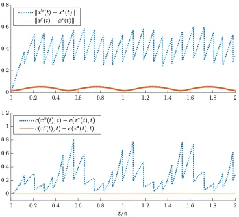
Figure 1.1 shows the curves of the distances to the optimal trajectorykxb(t) −x∗(t)k

and kxr(t) − x∗(t)k, and the objective value differencesc(xb(t),t) −c(x∗(t),t) and

(15)

[image:15.612.132.481.81.397.2]

Figure 1.1: The distances to the optimal trajectorykxb(t)−x∗(t)kandkxr(t)−x∗(t)k, and the objective value differencesc(xb(t),t) −c(x∗(t),t)andc(xr(t),t) −c(x∗(t),t)

of the two optimization schemes.

problem data much more frequently, and the resulting setpoints are able to keep track of the fast varying problem. While this toy example has a much simplified setting compared to practical scenarios, it demonstrates the benefits of time-varying optimization algorithms that can become significant in appropriate situations. Performance Evaluation of Time-Varying Optimization Algorithms

As previously discussed, the solutions provided by time-varying optimization algo-rithms are in general not optimal; instead one focuses on whether and how accurately the solutions cantrackthe optimal solution trajectory. Tracking performanceis cen-tral in evaluating time-varying optimization algorithms.

Let us consider the sampled problem (1.2), and denote x∗_τ_τ as a sequence of its (local) optimal solutions1. Suppose we run some time-varying optimization

1_{We choose}_x∗

(16)

algorithm and obtain a sequence of solutions denoted by (xˆτ)τ. So far in existing literature, three types of quantities have been proposed as metrics for tracking performance with respect to x_τ∗_τ.

1. The distance to the optimal solutionx∗_τ

eτ :=xˆτ− xτ∗ ,

where the norm can be arbitrary. When there are explicit equality or inequality constraints and the algorithm also generates dual iterates, we can also evaluate the distance between the primal-dual pairs. This metric has been analyzed in [64, 77, 84, 86–88, 95] for specific time-varying optimization algorithms and employed in [9, 29, 35, 36, 90] for specific applications.

2. The sub-optimality in terms of objective values. Comparison of objective values is standard for evaluating performance of online learning algorithms, and can be also employed in time-varying optimization. There can be two sub-categories in this type of metric:

a) The difference in objective values

eτ := cτ(xˆτ) −cτ(x∗_τ).

The notion of dynamic regret in online learning is closely related to this metric [48, 56, 68, 96, 99].

b) The ratio of objective values

rτ := cτ(xˆτ)

cτ(xτ∗) or r :=

Í

τcτ(xˆτ)

Í

τcτ(xτ∗).

Competitive ratio in online convex optimization can be viewed as a variant of this metric [4, 30, 63]. This metric can be employed in situations where the relative gap to the optimal objective value is more relevant than the absolute gap. On the other hand, one usually needs strong assumptions on the objective function to achieve a bounded competitive ratio.

When the iterates ˆxτ generated by the algorithm do not strictly satisfy the con-straints fτ(xˆτ) ≤0, we can use some meric function

φτ(x)=cτ(x)+Õ

i

g [fτ,i(x)]₊

(17)

3. The fixed-point residual

eτ := kxˆτ−Gτ(xˆτ)k,

where Gτ : Rn → Rn is a continuous map such that any fixed point of Gτ is an optimal solution (local or global) to (1.2) at time τ. This metric has been introduced and analyzed in [84].

We mention that, in existing literature, researchers have also proposed to compare ˆ

xτ with an optimal solution of the problem instance at the next time stepτ+1; in other words, metrics based on

xˆτ− x_τ∗₊₁

, cτ+₁ xˆτ

−cτ+1 x∗τ+1

_, cτ+1(xˆτ)

cτ+1 x_τ∗₊₁

, kxˆτ−Gτ+1(xˆτ)k

have also been proposed. It turns out that it doesn’t matter much whether we choose to compare ˆxτ withx_τ∗ or x∗_τ₊₁in the time-varying optimization setting₂; results on either one of the choices can usually be transferred to results on the other choice under appropriate conditions.

The three types of metrics are all reasonable quantitative characterizations of the tracking performance mathematically, and depending on specific scenarios where the time-varying optimization algorithms are applied, one can choose different metrics that are more suitable for application. In this thesis, we mostly use the first metric, the distance to the optimal trajectory, as the metric for tracking performance. 1.2 Review of Existing Works

In this section we give a brief and non-exhaustive review of some existing works on time-varying optimization and related topics.

Reference [77] is one of the early papers that consider time-varying optimization problems with a similar setting to the one in this thesis. The paper derived a tracking error bound of the running gradient descent algorithm for unconstrained time-varying convex optimization. Specifically, the paper showed that

lim sup τ→∞

xˆτ− x∗τ

≤

ρ

1− ρsup_τ

x∗τ− x∗_τ−₁

(1.5)

for the running gradient descent algorithm for time-varying unconstrained strongly convex problems, where

Λmin =inf_τ,x λmin

∇2cτ(x), Λmax =sup

τ,x λmax

∇2cτ(x),

(18)

ρ=max{|1−αΛ_min|,|1−αΛ_max|},

andα∈ (0,2/Λmax)is the step size. The paper also considered a special case where

the tracking errorkxˆτ−xτ∗ktends to zero asτ→ ∞. The tracking error bound (1.5) turns out to be one of the most fundamental results in time-varying optimization. Recent years have witnessed considerable advances in the theory and algorithms of time-varying convex optimization. [64] proposed a decentralized algorithm based on Alternating Direction Method of Multipliers for time-varying unconstrained con-sensus problems, and also derived a tracking error bound that is similar to (1.5). [86] proposed a running algorithm based on the consensus + innovations method for time-varying constrained consensus problems, and also showed a similar tracking error bound. [87] proposed and analyzed the double smoothing method based on the multiuser optimization algorithm in [60], which is one of the earliest time-varying optimization algorithms that treat explicit inequality constraints. [95] introduced auxiliary variables in the design of the running algorithm for time-varying uncon-strained consensus problems over directed networks, and showed convergence to a bounded tracking error. [84] proposed a unified framework for time-varying convex optimization using averaged operators, and derived tracking error bounds for sev-eral running algorithms. [16] proposed and analyzed a feedback-based time-varying optimization algorithm based on the primal-dual gradient method, which applies to logical or physical systems with feedback measurements. [34] proposed and analyzed a feedback-based method to regulate the output of a linear time-invariant dynamical system to the optimal solution of a time-varying convex optimization problem. [54] proposed a formulation of time-varying projected gradient dynamics by introducing the notion of temporal tangent cones, and showed existence of solu-tion to the resulting differential equasolu-tions. [15] developed an algorithmic framework for tracking fixed points of time-varying contraction mappings, and derived tracking error results in the situations where communication delays and packet drops lead to asynchronous algorithmic updates.

We would like to further expand on the results of [84] and [87]. In [84], the author considered the case where the time-varying optimization algorithm can be abstracted as

ˆ

xτ =Tτ xˆτ−1

_,

where for eachτ,Tτ :Rn→Rncan be represented as

(19)

for someaτ > 0 and some nonexpansive operatorGτ(i.e.,kGτ(x1)−Gτ(x2)k ≤ kx1− x2k), and the fixed point of the operatorTτ gives the optimal solutionx∗_τ. The paper showed that, ifσ := sup_τkx_τ∗ − x∗_τ−₁k < +∞ and X := sup_τsup_x∈_RnTτ(x) < +∞,

then the sequence(xˆτ)τ satisfies 1

K

Õ

τ=1

1−aτ

aτ kTτ(xˆτ−1) −xˆτ−1k

2 _≤ 1 K

x0ˆ −x₁∗

2

+σ(4X +σ).

In addition, in the special case whereTτ is a contraction mapping with a uniform contraction coefficientρ ∈ (0,1), it was shown that

xˆτ−₁−xτ∗

≤ ρτ−1kxˆ₀− x∗₁k+

1− ρτ−1

1−ρ σ.

The paper then applied this bound to several time-varying optimization algorithms. Especially, a bound on the fixed-point residual was established for the running projected gradient descent method that solves

min x∈X(t)c

(x,t),

where X(t) ⊂ _Rn _{is compact and uniformly bounded, and} _c_(·_,_t₎ _{is convex and} uniformly strongly smooth for eacht.

In [87], the authors considered the time-varying convex problem min

x∈X cτ(x) s.t. fτ(x) ≤0,

wherecτ :Rn→Ris convex, fτ :Rn →Rmhas convex components, andX ⊆Rnis convex and closed. The paper proposed a running version of the double smoothing algorithm [60] given by

ˆ

xτ = PX

ˆ

xτ−1−α∇xLν,τ (xˆτ−1,λˆτ−1)

_,

ˆ

λτ = PRm _ˆ

λτ−1+α∇λLτν,(xˆτ−1,λˆτ−1)

,

where the regularized LagrangianLν,_τ is defined by

L_τν,(x, λ):= cτ(x)+λT fτ(x)+ ν

2kxk

2₋

2kλk

2_.

The paper showed that, when the step sizeαis sufficiently small, there exists some

ρ <1 such that

lim sup k→∞

zˆτ−z?_τ₊₁

≤

1 1−ρsupτ

(20)

where ˆzτ = xˆτ,λˆτ, and z?_τ = x?_τ, λ?_τ denotes the saddle point of the regularized Lagrangian Lν,_τ (x, λ). The authors also considered how to implement the algo-rithm in a distribution manner when the cost and constraint functions have special structures.

Time-varying optimization is closely related to parametric optimizationthat has a long history [49, 73, 81]. The formulation of one-parametric optimization problems is almost the same as (1.1), wheretis regarded as a one-dimensional parameter that may or may not represent time. Path-following methods (also called continuation methods or homotopy methods) and their varients have been developed to solve these problems [3, 39, 43, 80, 85, 97]. A typical parametric optimization algorithm discretizes the parameter set [0,T] by 0 < t1 < . . . < tK ≤ T, and generates approximate solutions ˆxτ such that

e :=sup

τ kxˆτ− x ∗

(tτ)k =O(∆max), as ∆max→0,

where ∆_max = maxτ|tτ+1−tτ|. The theory of parametric optimization generally

focuses on the convergence rate of the approximation erroreas∆_max →0. In addi-tion, many parametric optimization algorithms consist of a predictor and a corrector: for eachτ = 1, . . . ,K, the corrector utilizes the problem data att = tτ to move the prediction produced by the previous iteration towards the optimal trajectory, and the predictor then estimates the tangent vectordz∗(t)/dtatt = tτto provide a prediction of the optimal solution at the subsequent parameter value. This predictor-corrector procedure assumes knowledge of how the cost and constraint functions evolve with time, which is different from the time-varying optimization setting discussed in this thesis. The theory and algorithms of parametric optimization provide important insights on and tools for the study of time-varying optimization.

We would also like to mention that, in online learning, theories on dynamic regret have been developed, which are closely related to time-varying optimization [21, 48, 51, 56, 62, 68, 96, 99]. In online learning, for each time step τ, a player chooses a strategy ˆxτfrom some feasible setXby an online learning algorithm, and suffers some loss cτ+1(xˆτ) 3. To evaluate the performance of the online learning

algorithm in the time-varying setting, the dynamic regret is proposed that compares the cumulative losses of the online player with the losses of the best possible 3_{We label the time indices in a fashion that is different from online learning literature but similar}

(21)

responses

K

Õ

τ=1

cτ xˆτ−1−cτ x∗τ.

Particularly, researchers are interested in bounding the growth rate of the dynamic regret asK → ∞ over a specific class of loss functions, and usually focus on the situations where the dynamic regret achieves sublinear growth.

For example, the pioneering paper [99] formulated the online convex programming problem in whichX ⊆ _Rnis convex and compact andcτis convex and differentiable for allτ. The paper proposed the online projected gradient descent algorithm whose iterations are given by

ˆ

xτ =PX[xˆτ−1−α∇cτ(xˆτ−1)].

The paper showed that, for the online projected gradient descent algorithm, the dynamic regret can be upper bounded by

K

Õ

τ=1

cτ xˆτ−1 −cτ xτ∗ ≤ 7R2

4α +

R α

K−1

Õ

τ=1

x∗_τ₊₁−x∗_τ

+

Gα

2 K, where

R:= sup x1,x2∈X

kx2−x1k, G:=sup

τ supx∈X

k∇cτ(x)k.

In [68], the authors considered an online learning problem whereX ⊆_Rnis convex and compact and the loss functioncτ is uniformly strongly convex, i.e., there exists

µ > 0 such that

cτ(x2) ≥cτ(x1)+∇cτ(x1)T(x2− x1)+ µ

2kx2−x1k

2_,

∀x1,x2 ∈ X.

It was shown that an improved bound on the dynamic regret can be derived for the online projected gradient descent algorithm when the step sizeαis sufficiently small:

K

Õ

τ=1

cτ xˆτ−1 −cτ xτ∗ ≤ G 1 1−ρ

K−1

Õ

τ=1

x_τ∗₊₁− x_τ∗

+

kxˆ0−x₁∗k

1− ρ

!

,

where

ρ=p

1−αµ, G= sup τ supx∈X

k∇cτ(x)k.

(22)

compact, each loss functioncτ :X → _Rwas assumed to beweakly pseudo-convex: there exists M > 0 such that

cτ x −cτ x_τ∗ ≤

    

   

M∇cτ(x)

T

x−xτ∗

k∇cτ(x)k ,

∇cτ(x)_,0,

0, ∇cτ(x)=0

for anyx ∈ Xand anyx_τ∗ ∈arg min_u∈Xcτ(u). The paper showed that, if the strategies ˆ

xτ are generated by theonline normalized gradient descentalgorithm

ˆ

xτ = PX[xˆτ−1−ηgτ], gτ :=

    

   

∇cτ(xˆτ−1) k∇cτ(xˆτ−1)k

, ∇cτ(xˆτ−1), 0, 0, ∇cτ(xˆτ−1)= 0,

whereηis some positive constant, then the following bound on the dynamic regret holds under certain conditions:

K

Õ

τ=1

cτ(xˆτ−1) −cτ(xτ∗) ≤ M 2η 4R

2₊_η2_K ₊₆_R

K−1

Õ

τ=1

x_τ∗₊₁− x∗τ !

,

where R := supx∈Xkxk. Further investigation of these examples and other related works suggests that, although time-varying optimization and online learning have different perspectives and settings, the mathematics behind the theories of dynamic regret can be very relevant for the research on time-varying optimization.

Time-varying optimization has also found its place in various applications. While the original formulation was for static problems, the network flow control algorithm in [67] is essentially implemented in a running fashion and can be easily extended to time-varying situations. In [29], the primal-dual saddle point dynamics was applied in time-varying wireless systems, with theoretical analysis on the tracking performance. In [9], the running version of the iterative soft-thresholding algorithm and its continuous-time counterpart for sparse signal recovery were analyzed under the time-varying setting. In [8], the authors proposed a running stochastic gradient descent method for topology tracking in social networks, though no theoretical guarantee on tracking performance has been provided.

(23)

double smoothing method [87] and a linearized power flow model for real-time oper-ation of distribution networks, and [14] presented a more comprehensive framework that can handle a wider range of controllable power devices. [52, 55] proposed continuous-time online algorithms that employ projected gradient dynamics on the power flow manifold.

1.3 Organization of the Thesis

Chapter 2: First-Order Algorithms for Time-Varying Optimization

In Chapter 2, we propose a first-order time-varying optmization algorithm, which we call the regularized proximal primal-dual gradient algorithm. The regulariza-tion comes in the form of a strongly concave term in the dual vector variable that is added to the Lagrangian function [50, 58, 60]. The strongly concave regular-ization term plays a critical role in establishing contraction-like behavior of the proposed algorithm. However, as an artifact of this regularization, existing works for time-invariant convex programs [60], time-varying convex programs [16], and for static nonconvex problems [50] could prove that gradient-based iterative methods approach an approximate KKT point. On the other hand, in Chapter 2 we provide analytical results in terms of tracking a KKT point (as opposed to an approximate KKT point) of (1.2) and provide bounds for the distance of the algorithmic iterates from a KKT trajectory. The bounds are obtained by finding conditions under which the regularized proximal primal-dual gradient step exhibits a contraction-like be-havior. The bounds are directly related to the maximum temporal variability of a KKT trajectory, and also depend on pertinent algorithmic parameters such as the step size and the regularization coefficient.

We then provide sufficient conditions for the existence of algorithmic parameters that guarantee bounded tracking error for sufficiently small sampling interval. From a qualitative standpoint, the sufficient conditions for the existence of feasible pa-rameters suggest that the problem should be “sufficiently convex” around a KKT trajectory to overcome the nonlinearity of the nonconvex constraints.

(24)

of the system of differential inclusions is analytically established; the continuous-time tracking error bound shares a similar form with the discrete-continuous-time tracking error bound. Then, we provide sufficient conditions for the existence of feasible algorithmic parameters, and also analyze the existence and properties of the optimal algorithmic parameters that minimize the tracking error bound.

Finally, we derive conditions under which the KKT points for a given time will always be isolated; that is, bifurcations or merging of KKT trajectories do not happen.

While most existing works on time-varying optimization focus on problems that are globally convex, our study does not assume global convexity of the objective and constraint functions, which can be particularly useful for time-varying nonconvex problems such as the time-varying optimal power flow problem. Part of these results have been reported in [88, 89].

Chapter 3: Second-Order Algorithms for Time-Varying Optimization

In Chapter 3, we consider second-order algorithms for time-varying optimization. By “second-order” algorithms, we mean that for eachτ, not only the current function value and gradient information is used, but also the exact or approximate curvature information is employed, which is similar to Newton and quasi-Newton methods in static optimization.

We first propose the approximate Newton method for a special case where the constraints in (1.2) appear in the form x ∈ X_τ for some closed and convexX_τ. The approximate Newton method is a natural extension of (quasi-)Newton method to the time-varying setting. It is shown that the tracking error is directly affected by how well we can approximate the curvature of the objective function cτ. We also propose a specific version of the approximate Newton method based on L-BFGS-B [26, 69] that handles box constraints.

(25)

program-ming [23] in the time-varying setting, with regularization on the dual variable just like the regularized proximal primal-dual gradient algorithm. We perform a direct analysis of the tracking error with respect to the optimal trajectory and discuss its implications.

Finally, we use a toy example to compare first-order and second-order methods, in order to have a better understanding of how to appropriately choose between these two types of methods in practical scenarios.

As mentioned in Section 1.2, parametric optimization is closely related to time-varying optimization, and many path-following algorithms utilize curvature infor-mation in a very similar fashion to the approximate Newton methods [39, 43, 49, 97]. On the other hand, parametric optimization generally focuses on whether and how fast the trajectory generated by path-following algorithms will converge to the opti-mal trajectory as the sampling interval goes to zero. This is different from our setting where we assume a given and fixed sampling interval, considering that the delays caused by computation, communication, etc. will prevent the sampling interval from being arbitrarily small in practice.

Similar to Chapter 2, we do not explicitly assume global convexity for the time-varying optimization problem in our study. Part of these results have been reported in [90, 91].

Chapter 4: Applications in Power System Operation

In Chapter 4, we discuss the application of time-varying optimization algorithms to power system operation, motivated by the consideration that batch solutions are inappropriate when one needs to optimize over a large number of distributed con-trollable devices to handle fast-timescale fluctuations and uncertainties introduced by distributed energy resources in future smart grids.

(26)

mismatch.

Then we present two real-time optimal power flow algorithms in detail. The first algorithm applies the regularized primal-dual gradient algorithm to the real-time operation of a distribution feeder. Specifically, we show how real-time measurement data can be naturally incorporated in the computation, and analyze the effect of employing approximate Jacobian of the implicit power flow map in the algorithm theoretically. The second algorithm applies the approximate Newton method with penalty functions to the time-varying optimal power flow problem. Second-order real-time optimal power flow method was first proposed by [90] and here we present the distributed implementation proposed in [91].

Chapter 5: Concluding Remarks on Future Directions

We conclude the thesis by remarks on some future directions that are worth explo-ration.

1.4 Notations and Terminologies

Sets and Functions

For any set A, its power set will be denoted by 2A, and the Cartesian product

A× · · · × A

| {z }

ntimes

will be denoted by An.

Let(Ai)_in₌₁be a finite sequence of sets, and letSbe a nonempty subset ofA1×· · ·×An. A mapπ :S →Ðn

i=1Aiis called a canonical projection if there existsj ∈ {1, . . . ,n}

such that

π(x1, . . . ,xn)= xj, ∀(x1, . . . ,xn) ∈S.

We denote_R₊ = [0,+∞)and_R₊₊= (0,+∞).

Suppose f : X →Y where X andY are any sets. For any subset A ⊆ Y, f−1[A]

denotes the preimage{x ∈ X : f(x) ∈ A}.

For a real-valued function f defined on an interval D ⊆ _R, we say that it is nondecreasing if∀x1,x2 ∈ D, x1 < x2⇒ f(x1) ≤ f(x2), and say that it is (strictly)

increasing if the inequality is strict. The notion of nonincreasing and (strictly) decreasing functions are defined similarly. We say that f is unimodal if there exists

x0 ∈ D such that f is strictly decreasing onD∩ (−∞,x0]and is strictly increasing onD∩ [x0,+∞).

(27)

For any x ∈ _R, bxc denotes the largest integernsuch thatn ≤ x, and dxe denotes the smallest integernsuch thatn ≥ x.

Linear Algebra

We use

x = (x1, . . . ,xn)=

       

x1 ... xn

       

to denote vectorx in_Rn. The Euclidean norm on_Rnwill be simply denoted by

kxk :=

v

t _n

Õ

i=1

x_i2, x ∈_Rn.

The identity matrix will be denoted byI, orIn∈Rn×nwhen the dimension needs to be specified to avoid confusion.

For any matrixM = Mi j ∈Rm×n. kMkdenotes the operator norm

kMk :=sup x_,0

kM xk kxk .

WhenM is a square matrix, we useλmax(M)andλmin(M)to denote the largest and

the smallest eigenvalues ofM respectively.

For two real symmetric matrix A and B, the expression A B means B− A is positive semidefinite, and A≺ BmeansB−Ais positive definite.

Real Analysis

For a topological space X and a subset A⊆ X, the interior of Awill be denoted by intA, and the closure of Awill be denoted by clA.

The closed unit ball in_Rncentered at the origin will be denoted byB_n. For any two subsets A,Bof_Rnand anyα, β ∈_R, we define

αA+βB :={αx+ βy : x ∈ A,y ∈ B}.

As an example,{x}+rB_nis the closed ball inRnof radiusrcentered at x.

Suppose f : X → _R∪ {+∞} where X is a topological space. We say that f is lower semicontinuous if lim infn→∞ f(xn) ≥ f(x)for any x ∈ X and any sequence

(xn) ⊂ X that converges to x. Equivalently, f is lower semicontinuous if {x ∈ X :

(28)

is upper semicontinuous if −f is lower semicontinuous. A function f : X → _R

is continuous if and only if it is both lower and upper semicontinuous. See [57, Section 12] for more details.

Let f :I →_Rbe a function defined on an interval I of_R. The essential supremum of f(t)overt ∈ I is defined by

ess sup t∈I

f(t):=infM ∈_R: Leb f−1[(M,+∞)] =0 , where Leb denotes the Lebesgue measure onR.

Let f :[a,b] →_Rm _{be a vector-valued function whose components are absolutely} continuous. Then there exists a Lebegue integrable function from [a,b] to Rm, which we denote byD f, such that

f(t) − f(a)=

∫ t

a

D f(s)ds

for allt ∈ [a,b], andD f is unique up to a Lebesgue null set. We will also denote d

dt f(t):= D f(t). Furthermore, f is Lipschitz continuous on[a,b]if and only if ess sup

t∈[0,T]

kD f(t)k < +∞,

or in other words,D f ∈ L∞([a,b]), and in this case, sup

t1,t2∈[a,b], t1,t2

kf(t2) − f(t1)k |t2−t1| =

ess sup

t∈[a,b] kD f(t)k.

See [44, Section 3.5] for more details. Differential Calculus

Let f :Rn→Rbe differentiable onRn. The gradient of f atx ∈Rnwill be denoted by∇f(x)which is ann-dimensional column vector. If f is twice differentiable, the Hessian of f at x ∈_Rnwill be denoted by∇2f(x).

Let f(x,y)be a function from_Rn×Y to_RwhereY is any set, and for some y0 ∈Y, f(x,y0) is differentiable with respect to x. The (partial) gradient of f(x,y) with

respect to xat(x0,y0) ∈Rn×Y will be denoted by∇xf(x0,y0). If f(x,y0)is twice

differentiable with respect to x, the (partial) Hessian of f(x,y)with respect to x at

(29)

Let f : Rn → Rm be a differentiable vector-valued function. We will denote its components by f1, . . . , fm. The Jacobian of f at x ∈Rnwill be denoted by

Jf(x):=

       

∇f1(x)T ... ∇fn(x)T

       

∈_Rm×n.

Let f(x,y) be a vector-valued function from Rn ×Y to Rm where Y is any set. Suppose for somey0 ∈Y, f(x,y0)is differentiable with respect to x. The (partial) Jacobian of f(x,y)with respect tox at(x0,y0) ∈Rn×Y will be denoted by

Jf,x(x0,y0):=

       

∇xf1(x0,y0)T ... ∇xfm(x0,y0)T

       

∈_Rm×n.

The following equalities can be shown by straightforward calculations.

Lemma 1.1. 1. Suppose f :Rn→ Rm is continuously differentiable. Then for any

x,y ∈_Rn_,

f(y)= f(x)+

∫ 1

0

Jf(x+θ(y− x))dθ

(y− x). (1.6) 2. Suppose f :Rn →Ris twice continuously differentiable. Then for anyx,y ∈Rn,

f(y)= f(x)+∇f(x)T(y− x)

+ 1

2(y−x) T

∫ 1

0

2(1−θ)∇2f(x+θ(y− x))dθ

(y− x).

(1.7)

Convex Analysis

LetC ⊆ _Rnbe a convex set. The indicator function ofCwill be defined and denoted by

IC(x)=

(

0, x ∈C, +∞, x_<C.

The relative interior ofCwill be denoted by relintC. The normal cone ofCatx ∈C

is defined by

NC(x):= {y ∈Rn : yT(z− x) ≤ 0, ∀z ∈C}.

(30)

projection of xintoC, and denote it by

PC(x):=arg min

y∈C

ky− xk.

Furthermore, we have the following proposition.

Proposition 1.1([20, Proposition 2.2.1]). SupposeC ⊆ _Rn_{is convex and closed.} 1. For anyx ∈_Rn,

y = P_C(x) ⇐⇒ (x− y)T(z− y) ≤ 0, ∀z ∈C ⇐⇒ x−y ∈ NC(y). 2. PC is nonexpansive, i.e.,kPC(x) − PC(y)k ≤ kx− yk for anyx,y ∈Rn.

For a convex coneC ⊆ _Rn_{, its polar cone is defined by}

C◦:= {y ∈_Rn: yTz ≤ 0, ∀z ∈C}.

For any subsetAofRn, its convex hull will be denoted by convA, and its affine hull will be denoted by affA.

Let f :Rn→R∪ {+∞}be a convex function. The domain of f is defined by dom(f):= {x ∈_Rn : f(x)< +∞}.

We say that f is proper if dom(f) is nonempty. We say that f is closed if the epigraph

epi(f):={(x,y) ∈Rn×R: y ≥ f(x)} is closed.

Proposition 1.2([82, Theorem 7.1]). A proper convex function f :Rn →R∪ {+∞} is lower semicontinuous if and only if it is closed.

The subdifferential of f at x0∈dom(f)is defined by

∂f(x0):=

u ∈_Rn: f(x) − f(x0) ≥ uT(x− x0), ∀x ∈Rn .

The definition indicates that ∂f(x0) is the intersection of a collection of closed

half-spaces inRn, and therefore is convex and closed.

Supposeg(x,y)is a function fromRn×Y toR∪ {+∞} whereY is any set, and for some fixed y0 ∈Y,g(x,y0)is a proper convex function of x. We denote the partial

subdifferential ofg(x,y)with respect tox at(x0,y0) ∈Rn×Y by

∂xg(x0,y0):=

(31)

C h a p t e r 2

FIRST-ORDER ALGORITHMS FOR TIME-VARYING

OPTIMIZATION

2.1 Problem Formulation

Let us consider the following time-varying optimization problem min

x∈Rn

c(x,t)+h(x,t)

s.t. fc(x,t)+ fnc(x,t) ≤ 0,

feq(x,t)=0.

(2.1)

Heret ∈ [0,T]labels time andT > 0 is a fixed constant that represents the length of the period we consider,c:Rn×R→ R,h :Rn×R→R∪ {+∞}, fc :Rn×R→Rm,

fc : Rn ×R → Rm and feq : Rn ×R → Rm

0

. For each fixed t ∈ [0,T], c(·,t),

fc(·,t), fnc(·,t)and feq(·,t)are twice continuously differentiable, fc(·,t)has convex components, and h(·,t)is a closed proper convex function with a closed domain. We denote the domain ofh(·,t)by

domt(h):= {x ∈_Rn :h(x,t)< +∞}.

In addition, we also assume that∇2_{x x}c(x,t),∇2_{x x}f_ic(x,t),∇2_{x x}f_inc(x,t)and∇2_{x x}f_jeq(x,t)

for each i = 1, . . . ,m and j = 1, . . . ,m0 are continuous over Rn × [0,T]. We let

fin := fc+ fnc.

We assume that (2.1) is feasible for allt ∈ [0,T], and that there exists a Lipschitz continuous trajectory of primal-dual pairz∗ =(x∗, λ∗, µ∗):[0,T] → Rn×Rm₊ ×Rm

0

such that for eacht ∈ [0,T], z∗(t)=(x∗(t), λ∗(t), µ∗(t))satisfies

(x∗(t), λ∗(t), µ∗(t)) ∈domt(h) ×Rm₊ ×Rm

0

, (2.2a)

−∇_xc(x∗(t),t) −

"

Jfin_,x(x∗(t),t)

Jfeq_,x(x∗(t),t) #T "

λ∗

(t) µ∗

(t)

#

∈∂_xh(x∗(t),t), (2.2b)

fin(x∗(t),t) ∈ N_Rm

+(λ ∗₍

t)), (2.2c)

(32)

Proposition 2.1. Supposex¯is a local minimum of the following optimization prob-lem

min x∈Rn

c(x)+h(x)

s.t. f(x) ∈ C,

(2.3) where c : Rn → R and f : Rn → Rp are continuously differentiable, h : Rn → R∪ {+∞} is a closed proper convex function with a closed domain, andC ⊆ Rp is a closed convex cone. Suppose the following constraint qualification condition is satisfied:

There is noλ∈ C◦\{0}such thatλTf(x¯)= 0and−Jf(x¯)Tλ∈ Ndom(h)(x¯). (2.4) Then there exists_λ¯ ∈ C◦such that

−∇c(x) −¯ Jf(x)¯ Tλ¯ ∈ ∂h(x),¯ (2.5a)

f(x¯) ∈ NC◦(λ¯). (2.5b)

The set of optimal Lagrange multipliers

Λ= λ¯ ∈ C◦: ¯λsatisfies(2.5) is convex and compact.

The proof is given in Appendix 2.A for completeness.

Remark 2.1. The constraint qualification in Proposition (2.4) can be viewed as a generalization of the Mangasarian-Fromovitz constraint qualification (MFCQ) [19]. Indeed, in the case whereh=0 andC =−_Rm₊ × {0}m0, we can prove that MFCQ is equivalent to (2.4). LetI ⊆ {1, . . . ,m}denote the index set of active constraints at

¯

x, and denoteE = {m+1, . . . ,m0}.

1. Suppose MFCQ holds at ¯x, and u ∈ _Rn _satisfies _J

fI(x¯)u < 0 and JfE(x¯)u = 0.

Suppose λ ∈ _Rm₊ ×_Rm0 satisfies λT f(x¯) = 0 and Jf(x¯)Tλ = 0. Then we have

λi = 0 fori <I ∪ E, and

0= λTJf(x)u¯ = λT_IJfI(x)u¯ +λ

T

EJfE(x)u¯ = λ

T

IJfI(x)u.¯

Considering that JfI(x)u¯ < 0 whileλI ≥ 0, we get λI = 0. Thus Jf(x)¯

T_λ ₌

JfE(x)¯

T_λ

E = 0. MFCQ requires thatJfE(x)¯ has linearly independent row vectors,

(33)

2. Suppose that MFCQ does not hold at ¯x. If the row vectors of JfE(x¯)are linearly

dependent, then there exists µ ∈ _Rm0_\{₀_} _{such that} _J fE(x¯)

T_µ ₌ _{0, and (2.4) is} obviously violated. If there is nou ∈_RnsatisfyingJfI(x¯)u < 0 andJfE(x¯)u= 0,

we let

S1 =

( "

JfI(x)¯

JfE(x¯) #

u:u ∈_Rn

)

, S2=

n

(z,0) ∈_R|I |×_Rm0 :z ∈ −_R₊₊|I |o.

Obviously S1 and S2 are convex sets, and since S1∩S2 = , by the separating hyperplane theorem, there exists some nonzero (v1,v2) ∈ R|I | ×Rm

0

such that

vT₁z ≥ 0 for allz ∈ −_R|I |₊₊, and

vT₁JfI(x)u¯ +v

T

2JfE(x)u¯ ≤ 0, ∀u ∈R

n_.

By setting u = JfI(x)¯

T_v

1 + JfE(x)¯

T_v

2 in the above inequality, we see that JfI(x¯)

T_v

1 + JfE(x¯)

T_v

2 = 0. On the other hand, vT₁z ≥ 0 for all z ∈ −R|I |₊₊ impliesv1 ≥ 0. We then see that if we defineλ∈Rm₊ ×Rm

0

byλI =v1,λE = v2

andλi =0 for anyi<I ∪ E, the constraint qualification (2.4) is violated byλ. We now see that the constraint qualification (2.4) is equivalent to MFCQ. Remark 2.2. In general, there can be multiple KKT points of (2.1) that move in Rn×Rm₊ ×Rm

0

as time proceeds, which form multiple trajectories that can appear, terminate, bifurcate or merge during the period (0,T). Reference [49] presented a very comprehensive theory of the structures and singularities of trajectories of KKT points for time-varying optimization problems. In [39], the authors show that strong regularity for generalized equations is a key concept for establishing the existence of Lipschitz continuous KKT trajectories over a given finite period. Here, we arbitrarily select one of these trajectories that is well defined and Lipschitz continuous for t ∈ [0,T], denote it by z∗(t), and mainly focus on this trajectory in

most part of our study.

As a special case of (2.1), if we seth(x,t)to be the indicator function

h(x,t)=

(

0, x ∈ X(t), +∞, otherwise,

(2.6)

(34)

following problem as a special case min x∈Rn

c(x,t)

s.t. fc(x,t)+ fnc(x,t) ≤ 0,

feq(x,t)=0,

x ∈ X(t),

(2.7)

and in this case, the subdifferential∂xh(x,t)is the normal cone NX(t)(x)as can be seen by

y ∈∂_xh(x,t) ⇐⇒ h(z,t) ≥ h(x,t)+yT(z−x), _∀z ∈_Rn ⇐⇒ 0≥ yT(z−x), _∀z ∈ X(t)

⇐⇒ y ∈NX(t)(x).

Proximal Operator

We define the proximal operator to a convex functiong :_Rk →_R∪ {+∞}by prox_g(x):=arg min

y∈Rk

g(y)+ 1

2ky−xk

2_. _(2.8)

The proximal operator can be viewed as a generalization of projection onto convex sets. Indeed, if we takeg to be the indicator function of a convex setC ⊆ _Rk, the proximal operator is just the projection ontoC.

The following lemma summarizes the properties of the proximal operator that will be frequently used in subsequent sections.

Lemma 2.1([74]). Letg :_Rk →_R∪ {+∞}be convex and proper. Then

1. prox_g(x)is well-defined for all x ∈_Rk.

2. y= prox_g(x)if and only if x−y ∈∂g(y).

3. prox_gis nonexpansive: for any x,y ∈_Rk,prox_g(x) −prox_g(y)

≤ kx−yk.

We can use the second property in Lemma 2.1 to rewrite two of the KKT conditions (2.2b) and (2.2c) equivalently in the form of a fixed-point equation

x∗(t)=prox_αh(·,t)

     

x∗(t) −α©

«

∇xc(x∗(t),t)+

"

Jfin_,x(x∗(t),t)

Jfeq_,x(x∗(t),t) #T "

λ∗₍

t) µ∗_(t)

#

ª ®

¬      

, (2.9a)

λ∗₍

t)= P_Rm

+

λ∗₍

(35)

2.2 Regularized Proximal Primal-Dual Gradient Algorithm

We first discretize the time domain [0,T] so that discrete-time algorithms can be proposed and implemented. Let ∆ > 0 be the sampling interval. Let T :=

{1,2, . . . ,bT/∆c}be the set of discrete time indices, and we denote

cτ(x)=c(x, τ∆), hτ(x)= h(x, τ∆),

f_τc(x)= fc(x, τ∆), f_τnc(x)= fnc(x, τ∆), f_τin(x)= fin(x, τ∆) fτeq(x)= feq(x, τ∆),

for each τ ∈ T. The sampled version of the KKT trajectoryz∗(t) will be denoted byz∗_τ =(x∗_τ, λ∗_τ, µ∗_τ)forτ ∈ T.

Let ˆz0 = (xˆ0,λˆ0,µˆ0) ∈ dom0(h) ×Rm₊ ×Rm

0

be the initial point. The regularized proximal primal-dual gradient algorithm produces a primal-dual pair (xˆτ,λˆτ,µˆτ) iteratively by

ˆ

xτ =proxαhτ

     

ˆ

xτ−1−α©

«

∇cτ(xˆτ−1)+

"

J_fin

τ (xˆτ−1) J_feq

τ (xˆτ−1)

#T "

ˆ

λτ−1

ˆ

µτ−1

#

ª ®

¬      

, (2.10a)

ˆ

λτ =PR₊m h

ˆ

λτ−1+ηα

f_τin(xˆτ−1) − λˆτ−1−λprior

i_,

(2.10b) ˆ

µτ = µˆτ−1+ηα f

eq

τ (xˆτ−1) − µˆτ−1−µprior (2.10c)

for each τ ∈ T. Here α > 0, η > 0, > 0, λprior ∈ _R₊m and µprior ∈ _Rm0 are parameters of the algorithm.

The regularized proximal primal-dual gradient algorithm is closely related to the following saddle point problem

min x∈Rn

max λ∈Rm+,µ∈Rm0

L_τ(x, λ, µ), (2.11)

whereL_τ(x, λ, µ)denotes the regularized Lagrangian defined by

L_τ(x, λ, µ)=cτ(x)+hτ(x)+λTfτin(x)+ µTfτeq(x)

−

2

λ−λ_prior

2 +

µ−µ_prior

2

. (2.12)

We can see that there is an additional term− 2

λ−λ_prior

2

+

µ− µ_prior

2

com-pared to the original Lagrangian function, which represents regularization that drives the dual variables towards λprior, µprior. Then, (2.10) can be viewed as applying a

(36)

update andηα for the dual updates respectively. The parameter then controls the amount of regularization on the dual variables. The constant vectorsλpriorandµprior can be viewed as prior estimates of the optimal dual variables, and can be set to zero if such prior estimates cannot be obtained1.

It can be seen that the regularized Lagrangian (2.12) is strongly concave with respect to the dual variables, which potentially improves the convergence behavior of primal-dual gradient methods. On the other hand, even if we solve the saddle point problem (2.11) exactly, the resulting solution will be in general different from the KKT points of (2.1), which suggests that there could be further sub-optimality introduced by regularization in the time-varying setting. This is indeed the case as will be seen in Section 2.3.

We denote the primal-dual pair produced by (2.10) as ˆzτ = (xˆτ,λˆτ,µˆτ). We define the norm

kzk_η :=

q

kxk2+η−1_kλ_k2+η−1_kν_k2

forz =(x, λ, ν) ∈ _Rn+m+m0. 2.3 Tracking Performance

The regularized proximal primal-dual gradient algorithm proposed in the previous section is expected to produce a sequence of primal-dual pairs that are sufficiently close to the KKT points for each time instant; in other words, the algorithm should be able to track the KKT points z∗_τ = (x_τ∗, λ_τ∗, µ∗_τ) for each τ. In this section, we study the tracking performance of the regularized proximal primal-dual gradient algorithm.

We define thetracking errorto be

zˆτ−z_τ∗

_η =

q

kxˆτ −xτ∗k2+η−1λˆτ −λ∗τ

2

+η−1_kµ_ˆ_τ₋ µ∗ τk2,

which represents the distance between the KKT point and the solution produced by (2.10); a small tracking error implies good tracking performance with respect to z_τ∗

τ. We are interested in factors that affect the tracking error, and especially conditions under which a bounded tracking error can be guaranteed.

1_{The dual update (2.10b) can also be equivalently written as}

ˆ

λτ =P_Rm +

h

ˆ

λτ−1+ηα

˜

f_τin(xˆτ−1) −λˆτ−1 i

with ˜f_τin(x)= f_τin(x)+λprior. In other words, we can also view (2.10b) as employing no prior estimate

(37)

Before proceeding, we first define some quantities that will be used in our analysis. Let

ση := sup t1,t2∈[0,T],

t1,t2

kz∗(t2) −z∗(t1)kη |t2−t1| =

ess sup t∈[0,T]

d dtz ∗₍ t) _η ,

i.e., the maximum speed of the KKT point with respect to the norm k · kη; hence

z∗_τ−z_τ−∗

1

_η ≤ ση∆for eachτ. We assume thatση >0 for some (and thus for any)

η > 0. Intuitively, the slowerz∗(t)moves, the more likely it is to obtain a smaller tracking error. We then define

Md := sup t∈[0,T]

"

λ∗₍

t) −λprior µ∗₍

t) −µprior

# , (2.13)

Mnc(δ):= sup t∈[0,T]

sup u:kuk≤δ

D2_{x x}

"

fnc(x∗(t)+u,t) feq(x∗(t)+u,t)

# , (2.14)

Mc(δ):= sup t∈[0,T]

sup u:kuk≤δ

D2_{x x}fc(x∗(t)+u,t)

, (2.15)

Lf(δ):= sup t∈[0,T]

sup u:kuk≤δ

"

Jfin_,x(x∗(t)+u,t)

Jfeq_,x(x∗(t)+u,t) # , (2.16)

D(δ, η):= √ηLf(δ)+ Mc(δ) sup t∈[0,T]

kλ∗(t)k. (2.17)

Here for a vector-valued f(x,t) that is twice continuously differentiable in x for a fixed t, we use D2_{x x}f(x,t) to denote the bilinear map that maps a pair of vectors

(h1,h2)to a vector whosei’th entry is given byhT₂∇2x xfi(x,t)h1, i.e., D2_{x x}f(x,t): (h1,h2) 7→

hT₂∇2_{x x}fi(x,t)h1

i,

andD2_{x x}f(x,t)

is defined by

D2_{x x}f(x,t)

:= sup

h1,h2,0

D2_{x x}f(x,t)(h₁,h₂)

kh1k kh2k = _k_h sup

1k=kh2k=1

D2_{x x}f(x,t)(h₁,h₂) .

Intuitively, D2_{x x}f(x,t)

characterizes the nonlinearity of function f with respect

to x at timet. Specifically, we have the following lemma, whose proof is given in Appendix 2.A.

Lemma 2.2. Lett ∈ [0,T]be fixed. Then for any x1,x2,

Jf,x(x2,t) − J_f,x(x1,t)

≤ kx2−x1k · sup

θ∈[0,1]

D2_{x x}f(x₁+θ(x₂−x₁),t) ,

(38)

and

f(x₂,t) − f(x₁,t) − Jf,x(x1,t)(x2−x1)

≤ 1

2kx2−x1k

2_· _sup

θ∈[0,1]

D2_{x x}f(x1+θ(x2−x1),t) .

(2.19)

The argumentδ ∈ (0,+∞) in the definitions (2.14)–(2.17) represents the radius of the ball centered atx∗(t), i.e., the local region aroundx∗(t)we are interested in. Let the “nonconvex Lagrangian component” be

Lnc(x, λ, µ,t):=c(x,t)+λTfnc(x,t)+µT feq(x,t), L_τnc(x, λ, µ):= Lnc(x, λ, µ, τ∆).

We also define

HLnc(u,t):=

∫ 1

0

∇2_{x x}Lnc(x∗(t)+θu, λ∗(t), µ∗(t),t)dθ, (2.20)

Hf_ic(u,t):=

∫ 1

0

2(1−θ)∇2_{x x}f_ic(x∗(t)+θu,t)dθ, (2.21) and

ρ(P)_{(δ, α, η,}₎

:= sup t∈[0,T],

u:kuk≤δ

I−αHLnc(u,t) 2

−α(1−ηα)

m

Õ

i=1 λ∗

i(t)Hfic(u,t)

,

ρ(δ, α, η, ):=

      

maxnρ(P)(δ, α, η, ),(1−ηα)2o +α(1−ηα) √

ηδMnc(δ) 2

+α2©

«

2 sup t∈[0,T],

u:kuk≤δ

ηI−HLnc(u,t)

D(δ, η)+D

2₍_{δ, η}₎ª ® ®

¬       

1/2 ,

κ(δ, α, η, ):= max

1, 1−ηα

ρ(δ, α, η, ), √

ηαLf(δ)

ρ(δ, α, η, )

.

Here, HLnc(u,t) is the averaged Hessian matrix of the “nonconvex Lagrangian

component” around x∗(t)along the vectoru, and Hfc

i (u,t)is the averaged Hessian

matrix of the convex part of the i’th constraint along the vector u. The quantity

ρ(δ, α, η, ), as we will show later, can be viewed as the contraction coefficient of a single step of the algorithm.

(39)

of these quantities will be employed again to study the continuous-time limit of the algorithm (2.10) in Section 2.4. The results in Theorem 2.1 will still follow if we replace all the supremum overt ∈ [0,T]by supremum overt ∈τT in the definitions

above.

The following lemma is critical in establishing the tracking error bound of the algorithm (2.10), whose proof will be presented in Appendix 2.A.

Lemma 2.3. Let τ ∈ T be arbitrary. Ifzˆτ−₁−z_τ∗

_η ≤ δ and zˆτ is generated by

(2.10), then

zˆτ−zτ∗

_η ≤ ρ(δ, α, η, )

zˆτ−₁−z∗τ

_η+κ(δ, α, η, )

√

ηαMd, (2.22) whereκ(δ, α, η, )is upper bounded by√2and satisfies

lim

α→0+κ(δ, α, η, )=1.

Now we present one of the main results of this chapter, which establishes the tracking error bound of the regularized proximal primal-dual gradient algorithm (2.10). Theorem 2.1. Suppose there existδ >0,α >0,η >0and > 0such that

ση∆≤ (1−ρ(δ, α, η, ))δ−κ(δ, α, η, )√ηαMd. (2.23a) Let the initial pointz0ˆ = (x0,ˆ λ0,ˆ µ0ˆ )be sufficiently close to the KKT pointz∗₁so that

z0ˆ −z₁∗

_η ≤ δ. (2.23b)

Then the sequence(zˆτ)τ∈T produced by the regularized proximal primal-dual gra-dient algorithm(2.10)satisfies

zˆτ−zτ∗

_η ≤

ρ(δ, α, η, )σ_η∆+κ(δ, α, η, )√ηαMd 1−ρ(δ, α, η, )

+ ρτ_{(δ, α, η, )} zˆ₀−z₁∗

_η−

ση∆+κ(δ, α, η, )√ηαMd 1−ρ(δ, α, η, )

(2.24)

for allτ∈ T.

Moreover, we have

lim α→0+κ

(δ, α, η, )=1 and κ(δ, α, η, ) ≤ √

(40)

Note that Lemma 2.3 asserts that if the radiusδis chosen such thatρ:= ρ(δ, α, η, )<

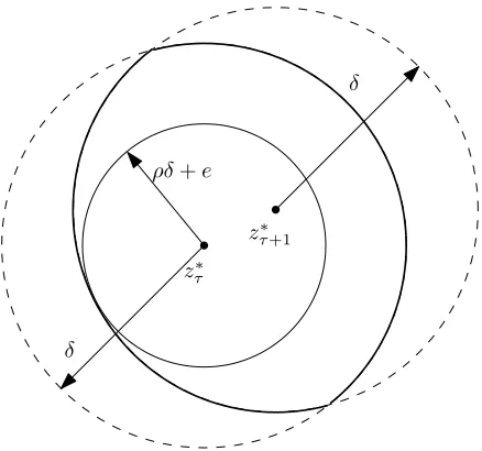
1, iteration (2.10) is an approximate local contraction with coefficient ρand error term e := κ(δ, α, η, )√ηαMλ. The idea of the proof of Theorem 2.1 is then based on showing that condition (2.23a) is sufficient to guarantee that the trajectory generated by the algorithm is confined within the contraction region at every time step. Note that (2.23a) implies

B(z_τ∗, ρδ+e) ⊆ B(z∗_τ₊₁, δ), (2.25) whereB(z, δ)is the ball centered atzwith radiusδ(with respect to the norm k · kη). Then, it is possible to show by induction that if ˆz0 ∈ B(z∗₁, δ), then ˆzτ−1 ∈ B(z∗τ, δ) for all τ. The idea of condition (2.25) is illustrated in Figure 2.1 and the formal proof of Theorem 2.1 is given below.

z∗_τ

z∗_τ₊₁

δ

[image:40.612.197.416.301.506.2]

ρδ+e

Figure 2.1: Illustration of condition (2.25). This condition is essentially on: (i) time-variability of a KKT point, (ii) extent of the contraction, and (iii) maximum error in each iteration. Note that in the error-less static case (i.e.,ση = e = 0), this condition is trivially satisfied.

Proof of Theorem 2.1. For notational simplicity, we just useρto denoteρ(δ, α, η, )

and use κto denote κ(δ, α, η, ). The condition (2.23b) guarantees that we can use Lemma 2.3 to get

z1ˆ −z₁∗

_η ≤ ρ

z0ˆ −z∗₁

_η+ κ

√