RBF-based multiscale control volume method for second order elliptic prob-lems with oscillatory coefficients
D.-A. An-Vo, C.-D. Tran, N. Mai-Duy and T. Tran-Cong
Computational Engineering and Science Research Centre, Faculty of Engineering and Surveying, The University of Southern Queensland, Toowoomba, Queensland 4350, Australia.
Abstract: Many important engineering problems have multiple-scale solutions. Thermal conductivity of composite materials, flow in porous media, and turbulent transport in high Reynolds number flows are examples of this type. Direct nu-merical simulations for these problems typically require extremely large amounts of CPU time and computer memory, which may be too expensive or impossible on the present supercomputers. In this paper, we develop a high order computa-tional method, based on multiscale basis function approach and integrated radial-basis-function (IRBF) approximant, for the solution of multiscale elliptic problems with reduced computational cost. Unlike other methods based on multiscale basis function approach, sets of basis and correction functions here are obtained through C2-continuous IRBF element formulations. High accuracy and efficiency of this method are demonstrated by several one- and two-dimensional examples.
Keywords: integrated radial basis functions, multiscale elliptic problems, Carte-sian grid, control volume method, multiscale method.
1 Introduction
medium characterised by equivalent properties, and coarse scale equations are pre-scribed in explicit form. Although upscaling techniques are effective, most of their applications have been reported for the case of periodic structures. As opposed to upscaling, multiscale methods consider the full problem with the original resolu-tion. The coarse scale equations are formed and solved numerically, where one constructs the basis functions from the leading order homogeneous elliptic equa-tion in coarse scale elements. The idea of using the non-polynomial multiscale approximation space rather than the standard piecewise polynomial space was first introduced by Babuška, Caloz, and Osborn (1994) for one-dimensional problems and by Hou and Wu (1997); Hou, Wu, and Cai (1999) for two-dimensional el-liptic problems. These methods have the ability to capture accurately the effects of fine scale variations without the need for using global fine meshes. Multiscale methods can be categorised into multiscale finite-element methods (MFEM) (e.g. Allaire and Brizzi (2005); Hou (2005)), mixed MFEM (e.g. Aarnes, Kippe, and Lie (2005); Arbogast (2002)) and multiscale finite-volume methods (MFVM) (e.g. Chu, Efendiev, Ginting, and Hou (2008); Jenny, Lee, and Tchelepi (2003)). Typ-ically, there are two different meshes used: a fine mesh for computing locally the basis function space, and a coarse mesh for computing globally the solution of an elliptic partial differential equation (PDE). The multiscale bases are independent of each other and their constructions can thus be conducted in parallel. In solv-ing the elliptic PDE, one may only need to employ a mesh that today’s computsolv-ing resources can efficiently and effectively handle. For two-scale periodic structures, Hou, Wu, and Cai (1999) have proved that the MFEM indeed converges to the cor-rect solution independent of the small scale in the homogenisation limit. Multiscale techniques require the solutions of elliptic PDEs which are achieved by means of discretisation schemes.
Re-cently, a local high order approximant based on 2-node IRBF elements (a smallest IRBF set ever used for constructing approximants) has been proposed by An-Vo, Mai-Duy, and Tran-Cong (2010, 2011a). It was shown that such IRBF elements (IRBFEs) lead to a C2-continuous solution rather than the usual C0-continuous so-lution. IRBFEs have been successfully incorporated into the subregion-collocation (An-Vo, Mai-Duy, and Tran-Cong, 2011b) and point-collocation (An-Vo, Mai-Duy, and Tran-Cong, 2011b; An-Vo, Mai-Duy, Tran, and Tran-Cong, 2013) formula-tion for simulating highly nonlinear flows accurately and effectively. We also use IRBFEs to model strain localisation in (An-Vo, Mai-Duy, Tran, and Tran-Cong, 2012).
This paper is concerned with the incorporation of IRBFEs and subregion colloca-tion (i.e. control-volume (CV) formulacolloca-tion) into the non-polynomial approximacolloca-tion space approach for solving one- and two-dimensional multiscale elliptic problems. Unlike other multiscale CV methods in the literature, sets of basis and correction functions in the present RBF-based multiscale CV method are obtained through highly accurate C2-continuous IRBFE-CV formulations. As a result, not only the field variable but also its first derivatives are reconstructed directly with high ac-curacy. This is an important issue since the first derivatives contain information of great practical interest, such as the stress distribution and heat flux in composite materials or the flow velocity field in porous media.
The remainder of the paper is organised as follows. Section 2 defines the problem. Section 3 and 4 briefly review the multiscale finite element and finite volume meth-ods, respectively, for the problem. The proposed method is described in Section 5 and numerical results are discussed in Section 6. Section 7 concludes the paper.
2 Problem definition
We consider the following multiscale elliptic problem
−∇·(λ∇u) = f in Ω, (1)
with appropriate boundary conditions.λ is a complex multiscale coefficient tensor; f a given function. Assume that the finest scale inλ is represented byε.
3 Multiscale finite-element methods (MFEM)
the small-scale features of the oscillatory coefficient tensorλ). The formulation of Hou and Wu (1997); Hou, Wu, and Cai (1999), namely the multiscale finite element method (MFEM), is based on a finite element framework where both the local and global problems are solved by a linear finite element method (LFEM). The MFEM is highly efficient and capable of capturing the large scale solution without resolv-ing all the small scale details. For the case of two-scale periodic structures, it has been proved in Hou, Wu, and Cai (1999) that the MFEM indeed converges to the correct solution independent of the small scale in the homogenisation limit. How-ever, for general cases e.g. non-periodic and random-scale media, the convergence of MFEM is not always guaranteed. In addition, there is an error gap between the MFEM solution and a corresponding fine scale reference solution. This error gap typically comes from two sources: (i) reduced problem boundary conditions for solving basis functions which is empirical even though an over-sampling technique has been proposed (Hou and Wu, 1997); and (ii) local homogeneous elliptic prob-lems for basis functions. Due to the latter the basis functions do not involve effects of the right hand side field f . The right hand side, in a manner similar to that in the MSFV method (discussed next), is only considered in the global coarse mesh system.
4 Multiscale finite volume (MSFV) method
Based on the multiscale basis function approach (Hou, Wu, and Cai, 1999; Hou and Wu, 1997), Jenny, Lee, and Tchelepi (2003) and Chu, Efendiev, Ginting, and Hou (2008) proposed the MSFV method for elliptic problems in subsurface flow simulation. Equation (1) governs the pressure field p as
−∇·(λ∇p) = f in Ω, (2)
with the boundary conditions ∇p·n=q and p(x) =g on∂Ω1 and ∂Ω2, respec-tively. Note that ∂Ω=∂Ω1∪∂Ω2 is the whole boundary of the domain Ωand n is the outward unit vector normal to ∂Ω. The mobility tensor λ (permeability, K, divided by the fluid viscosity, µ) is positive definite and the right-hand side f , q, and g are specified fields. The permeability heterogeneity is a dominant factor in dictating the flow behavior in natural porous formations. The heterogeneity of K is usually represented as a complex multiscale function of space. Resolving the spatial correlation structures and capturing the variability of permeability requires highly detailed description.
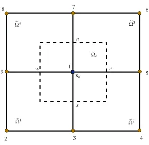
Hou, 2008). We present the latter here. A Cartesian grid of N×N is employed to represent the problem domain Ω (solid lines in Fig. 1), from which I (I = (N−2)×(N−2)) non-overlapping control volumesΩk associated with I interior
grid points xk(k∈[1,I]) are formed. This set of control volumes constitutes a grid
which is referred to as the coarse grid (dashed black lines in Fig. 1). In addition, letΩe be a collection of J cellsΩel (l∈[1,J],J= (N−1)×(N−1)) defined by the original N×N Cartesian grid (solid lines in Fig. 1). This set of J cells is referred to as the dual coarse grid. Note that these two grids can be much coarser than the underlying fine grid (dashed green lines in Fig. 1 wherein each dual cellΩel is dis-cretised by a local fine grid of n×n) on which the mobility field is represented. On each dual cellΩel, we seek the approximate solution p of p in the forme
pl ≈pel =
4
∑
i=1
pliφil, (3)
where pli andφilare the pressure value at and the basis function associated with the node xli, respectively, of the dual coarse cellΩel.
Unlike conventional discretisation methods, these basis functions{φil}4
i=1are gen-erated from solving the following leading order homogeneous elliptic equations on the dual coarse cellΩel,
∇·(λ∇φil) =0 in Ωel. (4)
Boundary conditions for (4) are derived from the requirement that φil(xlj) =δi j
(i,j∈[1,4]) and (4) be well-posed problems. Jenny, Lee, and Tchelepi (2003) employed the proposition in (Hou, Wu, and Cai, 1999) by solving reduced local one-dimensional problems to specify the boundary conditions for (4). The elliptic problems (4) inΩelwith such boundary conditions can be solved by any appropriate numerical method. In order to obtain a solution that depends linearly on the nodal pressures pli as in (3), we solve four elliptic problems, one for each nodal pressure. To derive a linear system for the nodal pressure values pk, we substitute expressions
(3) forp in the four dual cells associated with xe kinto equation (2) and integrate over
Ωk, which leads to
−
Z
Ωk
∇·(λ∇pe)dΩ=−
Z
Ωk
∇· λ∇ 4
∑
l=1 9
∑
i=1 φl
ipi !!
dΩ=
Z
Ωk
f dΩ, (5)
where the indices l and i refer to local dual cells and local nodal points, respectively, associated with xk and xk ≡x1 as shown in Fig. 2. Note that in the summation ∑9
toΩel (i.e. φil =0 otherwise). Applying the Gauss theorem to equation (5), one obtains
−
Z
∂Ωk
λ∇
∑
4l=1 9
∑
i=1 φl
ipi !!
·nkdΓ=
9
∑
i=1 pi
4
∑
l=1
Z
∂Ωk
−λ∇φil·nkdΓ=
Z
Ωk
f dΩ, (6)
where nkis the outward unit vector normal to∂Ωk. Equations (6) at a nodal point
xk (k∈[1,I]) can be written in matrix form as
Akipi=bk (7)
for the nodal pressure values pk with
Aki=
4
∑
l=1
Z
∂Ωk
−λ∇φl i
·nkdΓ (8)
and
bk=
Z
Ωk
f dΩ. (9)
We can reconstruct the fine scale pressure epl in each dual coarse cellΩel with pk
and the approximation (3). Implementing the reconstruction on the whole problem domainΩone obtains the fine scale pressure ep, which is an approximation of the pressure field p.
cells for basis functions. This step is a preprocessing step and has to be done once only. Furthermore, the construction of the fine scale basis functions is independent from cell to cell and therefore perfectly suited for parallel computation.
The MSFV method was firstly used for solving single-phase flow in homogeneous and heterogenous permeability fields in (Jenny, Lee, and Tchelepi, 2003). Jenny, Lee, and Tchelepi (2004) and Jenny, Lee, and Tchelepi (2006) extended the method to time dependent problems in incompressible two-phase flows where the explicit and implicit time integrations were presented respectively. Lunati and Jenny re-laxed the incompressible constraint in (Lunati and Jenny, 2006a) and compressible multiphase flow models were solved. It is important to note that until this stage of development the MSFV method basically was not designed to solve elliptic prob-lems with complex source terms and not appropriate to account for gravity and capillary pressure effects. The reason is that the basis functions and their linear combinations are solutions of local homogenous elliptic problems (4). The right hand side of the governing equation (2) is only taken into account in the coarse grid linear system (7). This led to the idea of introducing correction functions in (Lunati and Jenny, 2006b, 2008). Unlike basis functionsφil, correction functions plcare the solutions of local elliptic problems on the dual cells with the right hand side f , i.e.
∇·(λ∇plc) = f in Ωel. (10)
At the grid nodes xk which belong to Ωel, we impose plc(xk) =0. The boundary
conditions of (10) on the edge segments of the dual cell can be obtained in a man-ner similar to those in (4), i.e. by solving reduced local one-dimensional problems. It has been shown for a wide range of challenging test cases that these reduced problem boundary conditions provide a good localisation assumption. There exist scenarios, however, which demonstrate some limitations of these boundary condi-tions. Specifically, the MSFV solution with correction functions and global fine scale reference solution pf (pf is an approximation of p on the global fine grid) are
identical only if the basis and correction functions happen to capture the exact fine scale pressure solution on the interfaces of the dual coarse cells , i.e.
plf =
4
∑
i=1
pliφil+plc on ∂Ωel. (11)
It is desirable to approach boundary conditions for local elliptic problems via (11) instead of the reduced problem boundary conditions. Hajibeygi, Bonfigli, Hesse, and Jenny (2008) made it possible through an iterative framework based on a two-grid algorithm. At a step n with an initial pressure field ep(n), they perform several
e
p(sn). This smoothed pressure field yields the boundary values of correction
func-tions on each dual cell through (11) with plf replaced bype(sn), i.e.
plc=epls(n)− 4
∑
i=1
pliφil on ∂Ωel, (12)
where the boundary values of the basis functions φil on the dual cells are still ob-tained from the reduced problem boundary conditions. The boundary conditions (12) serve to solve the local problems (10) on the dual cells for the correction func-tions at step n. Then the nodal pressures pk are obtained through the solution of a
coarse grid system (Hajibeygi, Bonfigli, Hesse, and Jenny, 2008) and a new pres-sure field ep(n+1)is constructed via
e
pl(n+1)=
4
∑
i=1
pliφil+plc in Ωel. (13)
Again, we smooth pe(n+1) to yield a new smoothed field ep(sn+1) and repeat the
it-eration until convergence. It was shown by a series of examples in (Hajibeygi, Bonfigli, Hesse, and Jenny, 2008) that this iterative MSFV (iMSFV) method con-verges to the fine scale reference solution pf.
The iMSFV method relatively maintains the efficiency of MSFV method and has the possibility to approach the accuracy of corresponding fine scale solver. This method has been successfully applied to incompressible (Hajibeygi, Bonfigli, Hesse, and Jenny, 2008) and compressible (Hajibeygi and Jenny, 2009) multiphase flow in porous media. Recently, it is used adaptively (Hajibeygi and Jenny, 2011) and extended to simulate multiphase flow in fractured porous media (Hajibeygi, Kar-vounis, and Jenny, 2011).
5 Proposed RBF-based multiscale control-volume method
In this work we are interested in a one-parameter (ε) form of the multiscale elliptic problem (1), i.e.
−∇·(aε(x)∇u(x)) = f(x) in Ω (14)
of heat conduction in composite materials, u and a represent the temperature and thermal conductivity, respectively. In the case of flows in porous media, u is the pressure and a is the mobility field.
For the reasons mentioned above, the MFEM is an efficient method to capture the large scale solution but cannot produce the fine scale reference solution. In ad-dition, the method used in MFEM to determine the basis functions and solve the global coarse mesh problem is a linear finite element formulation. Note that there is an attempt to use a high-order method, e.g. the Chebyshev spectral method, to determine the basis functions in Hou and Wu (1997); Hou, Wu, and Cai (1999). They found that the accuracy of the final results is relatively insensitive to the accuracy of the basis functions. On the other hand, as described above, though possessing conservative property the MSFV method strongly resemble the MFEM and hence also cannot produce the fine scale reference solution. In contrast to the MFEM and the MSFV method, the iMSFV method (Hajibeygi, Bonfigli, Hesse, and Jenny, 2008) can produce the reference solution efficiently. However, a low order smoother has been used which results in a low-order accuracy relative to the exact solution. Moreover, like the MSFV method the iMSFV method requires a further reconstruction step to obtain a continuous velocity field for the solution of transport equations. It is pointed out in (Chen and Hou, 2002) that this is a compul-sory step to accurately solve the flow-transport-related applications, e.g. the single and multiphase flows through porous media.
It is desirable to develop a multiscale computational framework which can pro-duce the fine scale reference solution of elliptic problem (14) with high efficiency and accuracy. In the following, we propose a high-order conservative multiscale computational framework based on 2-node IRBFEs for solving (14). Unlike other multiscale computational frameworks, the proposed method can produce fine scale reference solutions efficiently with high accuracy. Furthermore, iterative solutions which converge to C2-continuous reference solutions are obtained in 2D problems. As a result, intrinsically continuous velocity fields are guaranteed automatically in flow-transport-related applications without the need for a reconstruction step. Be-cause of fundamental differences, the proposed method for 1D and 2D problems is presented independently, following a brief review of the two-node integrated-RBF elements in our discretisation scheme based on Cartesian grids.
5.1 Two-node integrated-RBF elements (IRBFEs)
Tanner (2007)) are utilised to represent the variation of the field variable and its derivatives, forming 2-node IRBFEs. It can be seen that there are two types of el-ements, namely interior and semi-interior elements. An interior element is formed using two adjacent interior nodes while a semi-interior element is generated by an interior node and a boundary node (Fig. 3).
5.1.1 Interior elements
1D-IRBF expressions for interior elements are of similar forms. Consider an inte-rior element,η∈[η1,η2], and its two nodes are locally named as 1 and 2. Letφ(η)
be a function andφ1,∂φ1/∂η, φ2 and ∂φ2/∂η be the values ofφ and ∂φ/∂η at the two nodes, respectively (Fig. 4(a)). The 2-node IRBFE scheme approximates the second-order derivative ofφ(η)using two multiquadric (MQ) functions whose centres are located atη1andη2
∂2φ
∂η2(η) =w1
q
(η−η1)2+a2
1+w2
q
(η−η2)2+a2
2=w1I
(2)
1 (η) +w2I
(2)
2 (η), (15)
where Ii(2)(η)conveniently denotes the MQ, wi and ai are the associated weight
and MQ-width at node i (i∈ {1,2}). We simply take ai=βh, where h is a grid size
andβ is a factor.
First-order derivative ofφand the functionφare approximated by integrating (15) with respect toη
∂φ
∂η(η) =w1I1(1)(η) +w2I2(1)(η) +C1, (16) φ(η) =w1I1(0)(η) +w2I2(0)(η) +C1η+C2, (17) where Ii(1)(η) =RIi(2)(η)dη, Ii(0)(η) =RIi(1)(η)dη, and C1 and C2 are the con-stants of integration. By collocating (17) and (16) atη1andη2, the relation between the physical space and the RBF coefficient space is obtained
φ1 φ2 ∂φ1 ∂η ∂φ2 ∂η
| {z } b φ =
I1(0)(η1) I2(0)(η1) η1 1 I1(0)(η2) I2(0)(η2) η2 1 I1(1)(η1) I2(1)(η1) 1 0 I1(1)(η2) I2(1)(η2) 1 0
| {z }
I w1 w2 C1 C2
| {z } b w
, (18)
whereφbis the nodal-value vector,I the conversion matrix, andw the coefficientb
owing to the presence of integration constants. Solving (18) yields
b
w=I−1φb. (19)
Substitution of (19) into (17), (16) and (15) leads to
φ(η) =hI1(0)(η),I2(0)(η),η,1iI−1φb, (20)
∂φ ∂η(η) =
h
I1(1)(η),I2(1)(η),1,0iI−1φb, (21)
∂2φ ∂η2(η) =
h
I1(2)(η),I2(2)(η),0,0iI−1φb. (22)
They can be rewritten in the form
φ(η) =ϕ1(η)φ1+ϕ2(η)φ2+ϕ3(η)∂φ1
∂η +ϕ4(η)∂φ2∂η, (23) ∂φ
∂η(η) =∂ϕ1
(η)
∂η φ1+∂ϕ2
(η)
∂η φ2+∂ϕ3
(η)
∂η ∂φ1∂η +∂ϕ4
(η)
∂η ∂φ2∂η, (24) ∂2φ
∂η2(η) =
∂2ϕ1(η) ∂η2 φ1+
∂2ϕ2(η) ∂η2 φ2+
∂2ϕ3(η) ∂η2
∂φ1 ∂η +
∂2ϕ4(η) ∂η2
∂φ2
∂η, (25) where{ϕi(η)}4i=1is the set of basis functions in the physical space. These
expres-sions allow one to compute the values ofφ,∂φ/∂η, and∂2φ/∂η2 at any pointη in[η1,η2]in terms of four nodal unknowns, i.e. the values of the field variable and its first-order derivatives at the two extremes (also grid points) of the element. For convenience, in the case ofη≡x, we denote
µi= ∂ϕ∂ i
x
x1+x2 2
, (26)
νi= ∂
2ϕ
i
∂x2 (x1), (27)
ζi= ∂
2ϕ
i
∂x2 (x2), (28)
and in the case ofη≡y, θi=∂ϕ∂ i
y
y1+y2 2
, (29)
ϑi=
∂2ϕ
i
∂y2 (y1), (30)
ξi=∂
2ϕ
i
∂y2 (y2), (31)
5.1.2 Semi-interior elements
As mentioned earlier, a semi-interior element is defined by two nodes: an interior node and a boundary node. The subscripts 1 and 2 are now replaced with b (for a boundary node) and g (for an interior grid node), respectively (Fig. 4(b)). Assume that the value ofφis given atηb. The conversion system can be formed as
φb
φg ∂φg
∂η
=
Ib(0)(ηb) Ig(0)(ηb) ηb 1
Ib(0)(ηg) I(
0)
g (ηg) ηg 1
Ib(1)(ηg) Ig(1)(ηg) 1 0
wb
wg
C1 C2
, (32)
which leads to
φ(η) =ϕ1(η)φb+ϕ2(η)φg+ϕ3(η)∂φ∂ηg, (33)
∂φ
∂η(η) =∂ϕ1
(η)
∂η φb+∂ϕ2
(η)
∂η φg+∂ϕ3
(η)
∂η ∂φ∂ηg, (34)
∂2φ ∂η2(η) =
∂2ϕ1(η) ∂η2 φb+
∂2ϕ2(η) ∂η2 φg+
∂2ϕ3(η) ∂η2
∂φg
∂η. (35)
It can be seen that the conversion matrix in (32) is under-determined and its in-verse can be obtained using the SVD technique (pseudo-inversion). Owing to the facts that point collocation is used and the RBF conversion matrix is not over-determined, the boundary conditionφbis imposed in an exact manner in the sense
that the error is due to the numerical inversion only and there is no intrinsic approx-imation errors such as those associated with “unconstrained" boundary conditions imposed by certain finite element methods (Burnett, 1987). For Neumann bound-ary conditions such as given surface traction or boundbound-ary pressure, other types of semi-interior elements have been proposed in (An-Vo, Mai-Duy, and Tran-Cong, 2011a) to which the reader is referred for details.
5.2 Proposed method for 1D problems
In a 1D domain, problem (14) reduces to
−d dx
aε(x)du(x)
dx
= f(x), x∈Ω, (36)
each interval or coarse cellΩel,Ωel = [xi−1,xi]with i∈[2,N]and l∈[1,N−1], an
approximation to the field variable u is sought in the form
ul(x) =φil−1(x)ui−1+φil(x)ui+ulc(x), (37)
where x∈Ωel, u
i−1=u(xi−1), ui=u(xi),φil−1(x)andφil(x)are the basis functions
associated with the nodes xi−1and xirespectively on the coarse cellΩel, and ulc(x)
is the correction function associated with the coarse cellΩel.
We employ subregion collocation to discretise (36). Each node xiwith i∈[2,N−1]
is surrounded by a control volume Ωi, Ωi = [xi−1/2,xi+1/2] as shown in Fig. 5. Integrating (36) over a control volumeΩi, one has
aε(xi+1/2) du
dx(xi+1/2)−a
ε(x i−1/2)
du
dx(xi−1/2) +
Z xi+1/2
xi−1/2
f dx=0. (38)
Taking (37) into account, one can express first derivatives in (38) in terms of nodal values of u. Unlike traditional discretisation methods, the basis functionsφil−1(x)
andφil(x)on a coarse cellΩel are not analytic functions (e.g. not polynomials), but local numerical solutions to the following differential equation
d dx
aεdφ
l k
dx
=0 (39)
with k∈ {i−1,i}and x∈Ωel. Boundary conditions for (39) are specified using the
condition φkl(xj) =δk jwith j∈ {i−1,i}. Likewise, the correction function ulc(x)
is a numerical solution to the following differential equation
−d dx
aεdu
l c
dx
=f (40)
with homogeneous boundary conditions ulc(xj) =0, j∈ {i−1,i}. Unlike (39) the
right hand side f of the governing equation (36) is involved in (40). Equation (39) needs to be solved twice while equation (40) needs to be solved once for the determination of the two basis functions and the correction function respectively on each coarse cell. A coarse cellΩelis discretised by a set of n points, called local fine
scale grid. Such a grid is used to capture the fine scale structure information of the solution. Let{η1=xi−1,η2, . . . ,ηn=xi}be a set of nodes of the local fine scale
grid. Similar to a coarse scale node, each fine scale nodeηmwith m∈[2,n−1]is
and (40) overΩm, one has respectively
aε(ηm+1/2) dφkl
dx (ηm+1/2)−a
ε(η m−1/2)
dφkl
dx (ηm−1/2) =0, (41) aε(ηm+1/2)du
l c
dx(ηm+1/2)−a
ε(η m−1/2)
dulc
dx (ηm−1/2) +
Z ηm+1/2
ηm−1/2
f dη=0. (42)
We propose to approximate the first-order derivatives in (41) and (42) by a 2-node IRBFE scheme, i.e. equation (24). Assuming that ηm−1 and ηm+1 are interior fine scale nodes, we can form two interior 2-node IRBFEs at ηm, i.e. elements
[ηm−1,ηm]and [ηm,ηm+1], to the left and right side ofηmrespectively. Applying
(24) with notation (26) to the element[ηm−1,ηm], one has
dφl k
dx (ηm−1/2) =µ1φ
l
k(ηm−1) +µ2φkl(ηm) +µ3
dφl k
dη(ηm−1) +µ4 dφl
k
dη(ηm), (43) dulc
dx (ηm−1/2) =µ1u
l
c(ηm−1) +µ2ulc(ηm) +µ3
dulc
dη(ηm−1) +µ4 dulc
dη(ηm). (44) Similarly, to the element[ηm,ηm+1], one has
dφkl
dx (ηm+1/2) =µ1φ
l
k(ηm) +µ2φkl(ηm+1) +µ3 dφkl
dη(ηm) +µ4
dφkl
dη(ηm+1), (45) dulc
dx (ηm+1/2) =µ1u
l
c(ηm) +µ2ulc(ηm+1) +µ3 dulc
dη(ηm) +µ4
dulc
dη(ηm+1). (46) Note that (43)-(46) will be slightly different at the coarse cell boundaries (also the coarse scale nodes) where (34) for semi-interior elements is used instead of (24). Substituting (43) and (45) into (41) yields
aε(ηm+1/2)µ2φkl(ηm+1) +aε(ηm+1/2)µ1−aε(ηm−1/2)µ2
φl k(ηm)
−aε(ηm−1/2)µ1φkl(ηm−1) +aε(ηm+1/2)µ4 dφkl
dη(ηm+1)
+aε(ηm+1/2)µ3−aε(ηm−1/2)µ4dφ
l k
dη(ηm)−a
ε(η
m−1/2)µ3 dφl
k
dη(ηm−1) =0. (47)
It can be seen from (47) that there are two unknowns, namelyφkl(ηm)and dφkl/dη(ηm),
associated with each nodal pointsηm(m∈[2,n−1]). Collection of (47) at all nodal
nodal points ηm, which is here achieved by imposing C2-continuous condition at
ηm, i.e. d2φl
k
dη2(ηm)
L
=
d2φl k
dη2(ηm)
R
, (48)
where(.)Lindicates that the computation of(.)is based on the element to the left
ofηm, i.e. element[ηm−1,ηm], and similarly subscript R denotes the right element
[ηm,ηm+1]. The left and the right of equation (48) are obtained via expression (25), noting (28) and (27) respectively, yielding
ζ1φl
k(ηm−1) +ζ2φkl(ηm) +ζ3
dφl k
dη(ηm−1) +ζ4dφ
l k
dη(ηm) =
ν1φl
k(ηm) +ν2φkl(ηm+1) +ν3 dφkl
dη(ηm) +ν4 dφkl
dη(ηm+1). (49) Collection of equations (47) and (49) at each and every fine scale nodesηm (m∈
[2,n−1]) with the associated boundary conditions leads to two systems of 2×
(n−2) equations for 2×(n−2) unknowns. These two systems are solved for the two basis functions onΩel. Unlike other conventional discretisation techniques, both the field variable and its first-derivative are considered in the present proposed technique, resulting C2-continuous solutions for the basis functions.
Similarly, at each fine scale nodeηm, substituting (44) and (46) into (42) and
im-posing C2-continuous condition at ηm lead to two equations for two unknowns
associated with ηm. Collection of these equations at all fine scale nodes with the
homogeneous boundary conditions results in a system of 2×(n−1)equations for 2×(n−1)unknowns. This system is solved for the correction function ulc associ-ated with the coarse cellΩel.
The set of basis and correction functions of the whole domainΩis used to represent the first derivatives in (38) in terms of coarse scale nodal values ui (i∈[2,N−1]).
Collection of equation (38) at all coarse scale nodes with the associated boundary conditions lead to a coarse scale system of N−2 equations for N−2 coarse scale nodal values of u. Consequently, the complete solution of problem (36) is con-structed on each and every coarse cellΩel via (37). It can be seen that the presently proposed multiscale method is conservative for both local and global problems.
5.3 Proposed method for 2D problems
We consider the coefficient tensor aε in the following form
aε =
aε(x) 0 0 bε(y)
where aε(x) and bε(y) are oscillatory functions involving a small scale ε. It is noted that the periodicity and scale separation assumptions of aε(x)and bε(y)are not necessary here. The two-dimensional equation (14) becomes
−∂ ∂x
aε(x)∂u
∂x
− ∂ ∂y
bε(y)∂u
∂y
=f(x,y). (51)
Here we are considering a particular class (51) of the general problem (14) for the convenience of presenting the main features of the proposed method. Extension of the proposed method to the general problem where aε is a full tensor requires con-sideration of a mixed derivative term and will be reported in an up-coming work. Nevertheless, the multiscale problem (51) does have important application in, e.g. two-dimensional semi-conductor quantum devices wherein there is a specific direc-tion oscilladirec-tion of the coefficients at each locadirec-tion in space and time. The readers are referred to (Wang and Shu, 2009) for the application of such device models in one-dimension.
A Cartesian grid system is employed to represent the problem domainΩin a man-ner similar to that in the MSFV method (e.g. Fig. 1). Integrating (51) over a control volumeΩk and then applying the Green’s theorem in plane, one has
− Z Ωk ∂ ∂x
aε(x)∂u
∂x
+ ∂
∂y
bε(y)∂u
∂y
dΩ=
−
Z
∂Ωk
aε(x)∂u
∂xdy+
Z
∂Ωk
bε(y)∂u
∂ydx=Akfk, (52) where Akis the area ofΩk and
fk=
1 Ak
Z
Ωk
f dΩ. (53)
Approximating the line integrals in (52) by the midpoint rule, one obtains
−
aε(x)∂u
∂x
e
−
aε(x)∂u
∂x
w
∆y−
bε(y)∂u
∂y
n
−
bε(y)∂u
∂y
s
∆x=Akfk,
(54)
where∆xand ∆yare the coarse grid spacing in x and y direction respectively; and
To estimate the first-order derivatives of u in (54) we consider the dual coarse cells
e
Ωl in a 2D computational domain as shown in Fig. 1. We seek the approximation
for the field variable u on eachΩel in the form ul(x) =
4
∑
i=1 φl
i(x)ui+ulc(x), (55)
whereφil(x)is the basis function associated with a coarse scale node xiand i∈[1,4]
is the local index of the four nodes of a coarse cellΩel, ui=u(xi), and ulc(x)is the
correction function associated with a coarse cell Ωel. As explained earlier via (4)
and (10), these basis functions and correction function are similarly local numerical solutions of problem (51) onΩel without and with right-hand side, respectively, i.e. −∂
∂x
aε(x)∂φ
l i ∂x − ∂ ∂y
bε(y)∂φ
l i
∂y
=0, (56)
−∂ ∂x
aε(x)∂u
l c ∂x − ∂ ∂y
bε(y)∂u
l c
∂y
= f(x,y). (57)
Boundary conditions for (56) are ∂
∂x
aε(x)∂φ
l i
∂x
=0 on ∂Ωelx, (58)
∂ ∂y
bε(y)∂φ
l i
∂y
=0 on ∂Ωely, (59)
and for (57) are ∂
∂x
aε(x)∂u
l c ∂x = ∂ ∂x
aε(x)∂uf
∂x
on ∂Ωelx, (60)
∂ ∂y
bε(y)∂u
l c ∂y = ∂ ∂y
bε(y)∂uf
∂y
on ∂Ωely, (61)
where∂Ωelxand∂Ωelydenote the x- and y-segments, respectively, of the boundary of a dual cellΩel and uf is a reference solution on the global fine scale grid. A method
to create a fine scale reference solution uf will be presented in the following section.
At the dual-grid nodes xiwhich belong toΩel,φlj(xi) =δji( j∈[1,4]) and ulc(xi) =0.
The first-order derivatives of u in (54) can now be estimated by using expressions (55) for ul in the four dual coarse cells associated with a grid node xk (Fig. 2).
Specifically, we use local indices of l (l∈[1,4]) and i (i∈[1,9]) for local dual coarse cells and local coarse nodes, respectively, associated with xk and xk ≡x1 (Fig. 2) to obtain
∂ u ∂x e = ∂φ 2 1
∂x (xe)u1+ ∂φ2
5
∂x (xe)u5+ ∂u2c
∂x (xe) = ∂φ3
1
∂x (xe)u1+ ∂φ3
5
∂x (xe)u5+ ∂u3c
∂x (xe), (62) ∂ u ∂x w = ∂φ 1 9
∂x (xw)u9+ ∂φ1
1
∂x (xw)u1+ ∂u1c
∂x (xw) = ∂φ4
9
∂x (xw)u9+ ∂φ4
1
∂x (xw)u1+ ∂u4c
∂x (xw), (63) ∂ u ∂y n = ∂φ 3 1
∂y (yn)u1+ ∂φ3
7
∂y (yn)u7+ ∂u3c
∂y (yn) = ∂φ4
1
∂y (yn)u1+ ∂φ4
7
∂y (yn)u7+ ∂u4c
∂y (yn), (64) ∂ u ∂y s = ∂φ 1 3
∂y (ys)u3+ ∂φ1
1
∂y (ys)u1+ ∂u1c
∂y (ys) = ∂φ2
3
∂y (ys)u3+ ∂φ2
1
∂y (ys)u1+ ∂u2c
∂y (ys). (65)
We substitute (62)-(65) into (54) to obtain the discretised equation at a coarse node xk. Collection of the discretised equations at all coarse nodes leads to a linear
system to be solved for the coarse scale nodal values uk, k∈[1,N−2×N−2].
Consequently, the solution for u in each dual coarse cell Ωel is reconstructed via uk and the approximation (55). By implementing the reconstruction on the whole
problem domainΩ, the global solution for u is obtained.
It should be noted that the current computational framework for u depends strongly on the boundary conditions of local problems for the determination of the correction functions, i.e. (60) and (61), which unfortunately require a priori knowledge of uf.
To obtain the fine scale reference solution uf one typically has to directly resolve
all the small scale features of a multiscale problem. In the following section, we avoid this costly and even impossible task by proposing a conservative fine scale solver based on 2-node IRBFEs.
5.3.1 Fine scale C2-continuous conservative solver
procedure in obtaining (54), one has
−
aε(x)∂u
∂x
e
−
aε(x)∂u
∂x
w
δy−
bε(y)∂u
∂y
n
−
bε(y)∂u
∂y
s
δx=APfP,
(66)
whereδxandδyare fine grid spacing in x and y direction respectively; the subscripts
e,w,n and s are now used to indicate that the flux is estimated at the intersections of the fine grid lines with the east, west, north and south faces of the control volume ΩP, respectively (Fig. 6); and AP is the area ofΩP and fP= A1P
R
ΩP f dΩ. Unlike
(62)-(65), the fluxes are presently computed via 2-node IRBFEs defined over line segments between P and its neighbouring grid nodes (E,W,N and S). There are 4 IRBFEs associated with a control volumeΩP. Assuming that PE, W P are interior
elements and making use of (24), noting (26), one obtains fluxes in the x-direction as ∂ u ∂x e
=µ1uP+µ2uE+µ3∂
uP
∂x +µ4 ∂uE
∂x with x1≡xP and x2≡xE, (67)
∂
u ∂x
w
=µ1uW+µ2uP+µ3∂
uW
∂x +µ4 ∂uP
∂x with x1≡xW and x2≡xP. (68)
Expressions for the flux at the faces y=ynand y=ysare of similar forms obtained
by using PN and SP, assumed as interior elements, and making use of (24), noting (29), ∂ u ∂y n
=θ1uP+θ2uN+θ3∂
uP
∂y +θ4 ∂uN
∂y with y1≡yP and y2≡yN, (69)
∂
u ∂y
s
=θ1uS+θ2uP+θ3∂
uS
∂y +θ4 ∂uP
∂y with y1≡yS and y2≡yP. (70)
(67)-(70) may change if PE, W P, PN, and SP are semi-interior elements where (34) is used instead of (24).
Substituting (67)-(70) into (66), one has
G[x]
uuWP
uE +G[y]
uuSP
uN +D[x]
∂uW ∂x ∂uP ∂x ∂uE ∂x +D[y]
∂uS
∂y ∂uP
∂y ∂uN
∂y
where
G[x]=− −aε(xw)µ1 aε(xe)µ1−aε(xw)µ2 aε(xe)µ2
δy, (72)
G[y]=− −bε(ys)θ1 bε(yn)θ1−bε(ys)θ2 bε(yn)θ2
δx, (73)
D[x]=− −aε(xw)µ3 aε(xe)µ3−aε(xw)µ4 aε(xe)µ4 δ
y, (74)
D[y]=− −bε(ys)θ3 bε(yn)θ3−bε(ys)θ4 bε(yn)θ4
δx. (75)
It can be seen from (71), there are three unknowns, namely uP,∂uP/∂x and∂uP/∂y,
at a grid node P. To solve (71), two additional equations are needed and devised here by enforcing C2-continuity condition at P in x- and y-directions, i.e.
∂2u
P
∂x2
L
=
∂2u
P
∂x2
R
, (76)
∂2u
P
∂y2
B
=
∂2u
P
∂y2
T
, (77)
where(.)Lindicates that the computation of(.)is based on the element to the left of
P, i.e. element W P, and similarly subscripts R,B,T denote the right(PE), bottom
(SP)and top(PN)elements. Making use of (25) with noting (27) and (28) for (76) and (30) and (31) for (77), one has
ζ1uW+ζ2uP+ζ3∂
uW
∂x +ζ4 ∂uP
∂x =ν1uP+ν2uE+ν3 ∂uP
∂x +ν4 ∂uE
∂x , (78)
ξ1uS+ξ2uP+ξ3∂
uS
∂y +ξ4 ∂uP
∂y =ϑ1uP+ϑ2uN+ϑ3 ∂uP
∂y +ϑ4 ∂uN
∂y . (79) In compact forms, (78) and (79) can be rewritten as
C[x]h uW uP uE ∂u∂xW ∂u∂xP ∂u∂xE iT
=0, (80)
C[y]h uS uP uN ∂u∂yS ∂∂yuP ∂∂uyN iT
=0, (81)
with
C[x]= [ ζ1 ζ2−ν1 −ν2 ζ3 ζ4−ν3 −ν4 ], (82)
C[y]= [ ξ1 ξ2−ϑ1 −ϑ2 ξ3 ξ4−ϑ3 −ϑ4 ]. (83)
fine grid leads to a global fine scale system,
G[x]+G[y] D[x] D[y]
u ux
uy
=R, (84)
C[x]
u ux
=0, (85)
C[y]
u uy
=0, (86)
where G[•],D[•]and C[•]result from the assembly of G[•],D[•]and C[•]respectively; u,ux and uy are global vectors of values of u at all nodal points and its x- and
y-partial derivatives at interior grid nodes; and R collects the right hand side of (71), which results from the application of (71) at fine scale interior grid nodes.
Instead of directly solving the large fine scale system (84)-(86) for the fine scale reference solution uf, we propose a line-relaxation (LR) scheme to smooth a
tem-porarily guessed approximate fine grid solution. Assuming that u(t)and u(yt)are a
temporarily guessed solution, an iterative strategy in two stages for smoothing is proposed as
G[x]+diag(G[y]) D[x] C[x]
u ux
γ+1/2
=
R− G[y]−diag(G[y]) D[y]
u uy
γ
0
, (87)
G[y]+diag(G[x]) D[y] C[y]
u uy
γ+1
=
R− G[x]−diag(G[x]) D[x]
u ux
γ+1/2
0
, (88)
where[ u ux uy ]γ is the approximate solution after the γ smoothing step and
[ u uy ]0= [ u(t) uy(t) ], diag(G[x])is the diagonal of G[x]. Owing to the fact that
of massively parallel computation. Note that the present C2-continuous IRBFE-LR solver is convergent, but for large problem the rate is extremely slow. In our frame-work, however, only a few LR-steps are required to smooth the temporarily guessed approximate solution. The smoothed fine grid solution then serve to estimate tem-porary boundary conditions for correction functions via (60) and (61) instead of the fine scale reference solution uf. To ensure that these temporary boundary
condi-tions approach the condicondi-tions (60) and (61) an iterative algorithm is used. Such an algorithm is presented next.
5.3.2 Iterative algorithm
We present here an iterative algorithm to improve the localised boundary conditions of the correction functions. Such boundary conditions do not depend on uf. Instead
of requirements (60) and (61), we employ an iterative improvement ∂
∂x a
ε(x)∂ulc
(t)
∂x
!
= ∂
∂x a
ε(x)∂u(st)
∂x
!
on ∂Ωelx, (89)
∂ ∂y b
ε(y)∂ulc
(t)
∂y
!
= ∂
∂y b
ε(y)∂u(st)
∂y
!
on ∂Ωely ∀l∈[1,J]. (90) The superscript(t)denotes an iterative step and
h
u(st) ∂u
(t)
s
∂x ∂u
(t)
s
∂y i
=Snsh u(t) ∂u(t)
∂x ∂u
(t)
∂y i
(91)
is a smoothed fine scale approximate solution, where S is the proposed C2-continuous IRBFE-LR smoothing operator, i.e. (87) and (88), ns the number of smoothing
steps, and h
u(t) ∂∂xu(t) ∂u∂(yt) i
is the temporary solution which is constructed on each dual coarse cellΩel as ul(t)=
4
∑
i=1 φl
iu
(t)
i +ulc
(t−1)
, (92)
∂ul(t) ∂x =
4
∑
i=1 ∂φl
i
∂x u
(t)
i +
∂ulc(t−1)
∂x , (93)
∂ul(t) ∂y =
4
∑
i=1 ∂φl
i
∂y u
(t)
i +
∂ulc(t−1)
∂y ∀l∈[1,J]. (94)
algorithm is given below.
(1)Initialise
h
u(t=0) ux(t=0) u(yt=0) i
(2)∀l,∀i: omputebasisfuntions φ
l
i,equations(56) withboundary onditions
(58), (59) by aC 2
-ontinuous IRBFE-CV method (An-Vo, Mai-Duy, and Tran-Cong, 2011a)
(3)fort=1 tonumber ofiterations{ (3i)
h
u(st−1) u(xts−1) u
(t−1)
ys
i
=h u(t−1) ux(t−1) u(yt−1) i
(3ii)fori=1to ns {
h
u(st−1) u(xts−1) u
(t−1)
ys
i
=Sh us(t−1) u(xts−1) u
(t−1)
ys
i
;
smooth-ing step
}
(3iii)∀l: omputeorretionfuntionsu
l c
(t−1)
;basedonu
(t−1)
s ,equations
(57) with boundary onditions (89) and (90) by a C 2
-ontinuous IRBFE-CV
method (An-Vo,Mai-Duy,and Tran-Cong, 2011a)
(3iv)Calulate righthand sideofthe oarsegriddisretised system (3v) Solveoarse system
(3vi) Reonstrut
h
u(t) u(xt) u(yt) i
,equations(92)-(94)
(3vii)Calulate onvergenemeasures(CMs)through CM(u) =ku
(t)−u
f k2
kuf k2
CM(ux) =
ku(xt)−uxf k2
kuxf k2
CM(uy) =
ku(yt)−uyf k2
kuyf k2
}.
First, the fine scale field is initialised to zero. Then, all basis functions are computed and the right-hand side of equation (51) is integrated over each coarse volume. These steps have to be performed only once and are followed by the main iteration loop. At the beginning of each iteration, ns smoothing steps are applied and the
5.3.3 Deferred correction of coarse grid fluxes
In the coarse grid flux expressions, namely (62)-(65), there are required first-derivative values of basis functions and correction functions at the control volume faces. The former needs to be computed only once at the preprocessing stage and be fixed throughout the iteration loop. The latter, however, need to be updated at each itera-tion via the numerical differentiaitera-tion of correcitera-tion funcitera-tions. This differentiaitera-tion is usually resulted in a considerable numerical error. Here we propose a deferred cor-rection strategy to obtain the coarse grid fluxes accurately without the need of the numerical differentiation of correction functions. Consider an east control volume face at an iteration level t, instead of using (62) we compute the flux value as
∂
u ∂x
(t)
e
=∂φ
2 1 ∂x (xe)u
(t)
1 + ∂φ2
5 ∂x (xe)u
(t)
5 +∆f
(t−1)
e =∂φ
3 1 ∂x (xe)u
(t)
1 + ∂φ3
5 ∂x (xe)u
(t)
5 +∆f
(t−1)
e ,
(95)
where∆fe(t−1)is the correction term at e which is a known value derived from the
smoothed fine scale field, i.e.
∆fe(t−1)= ∂
u ∂x
(t−1)
e
−
∂φ2 1 ∂x (xe)u
(t−1)
1 +
∂φ2 5 ∂x (xe)u
(t−1)
5 = ∂ u ∂x
(t−1)
e
−
∂φ3 1 ∂x (xe)u
(t−1)
1 +
∂φ3 5 ∂x (xe)u
(t−1)
5
. (96)
Since the proposed C2-continuous fine scale solver is used the smoothed fine scale field includes not only the field variable but also its first partial derivatives. As a result, the value(∂u/∂x)(et−1) is explicitly given without the need of numerical differentiation. The flux values at other control-volume faces can be computed in a similar manner. It can be seen that via this correction strategy the coarse grid fluxes are matched with the fine scale smoothed field.
6 Numerical results
local fine grids on the coarse cells are mapped to[0,1]in 1D problems and[0,1]2 in 2D problems and the grid spacing is denoted as h.
In each problem, two grid refinement strategies are employed. The first strategy, Strategy 1, keeps the coarse grid fixed while refining the local fine grids. In contrast, the second strategy, Strategy 2, keeps the local fine grids fixed while refining the coarse grid. The numerical results are compared with those obtained by the MFEM (Hou, Wu, and Cai, 1999).
The factor of the MQ-width is chosen asβ =15 throughout the computation. We assess the numerical performance of the proposed method through two measures: (i) the relative discrete L2error defined as
Ne(α) =
r
∑M i=1
αi−αi(e) 2
r
∑M i=1
α(e)
i
2 (97)
where M is the number of test points,α denotes the field variable u and its deriva-tives and (ii) the convergence ratesγwith respect to the two grid refinement strate-gies defined via the error norm behaviours O(hγ) and O(Hγ) for the Strategy 1 and 2 respectively. The convergence rates are calculated over 2 successive grids (point-wise rate) and also over the whole set of grids used (average rate).
6.1 One-dimensional examples
6.1.1 Example 1
Consider a model 1D problem (36) with
aε(x) = 1
2+x+sin(2πx/ε), f =x, Ω= [0,1], (98)
and homogeneous Dirichlet boundary conditions u(0) =u(1) =0.
FEM give convergence rates of 4.0267 and 2.0253 respectively. It can be seen that the use of high order approximants in the form of IRBFEs thus helps capture the fine scale physics and hence produce highly accurate solutions.
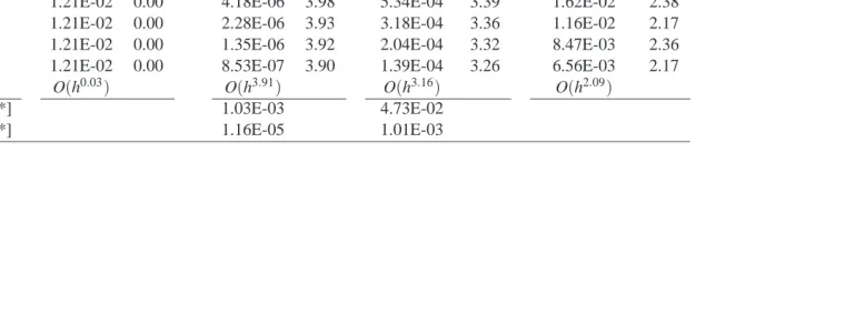
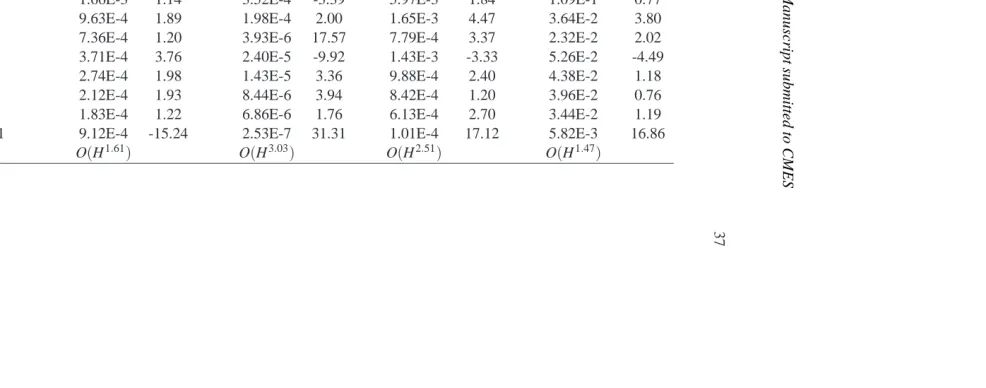
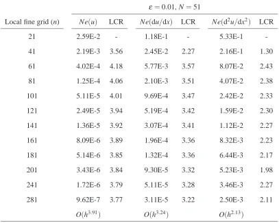
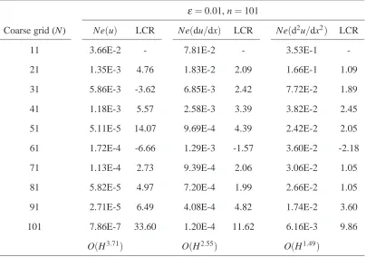
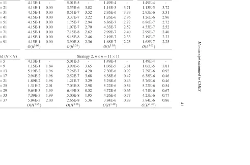
The coarse scale solution at the coarse grid points is obtained by a conservative CV method where the fluxes are estimated by the obtained shape and correction functions. In order to have a good consistent measure of accuracy, error norms in all cases are computed using the same 10,001 test points where the fine scale solution is recovered via (37). Table 1 presents convergence behaviour associ-ated with Strategy 1 where a fixed coarse scale grid of 10 elements and a series of 21,41, . . . ,181 local fine grids are used. The present method converges mono-tonically while MFEM does not converge. It was pointed out in (Hou and Wu, 1997; Hou, Wu, and Cai, 1999) that the accuracy of the shape functions does not have much effect on the overall accuracy of MFEM. The present approach achieves convergence rates of 3.91, 3.16, and 2.09 for the field variable, its first, and sec-ond derivatives respectively. In comparison to multiscale discontinuous Galerkin method proposed by Wang, Guzman, and Shu (2011), in terms of L2 error, the present method yields two orders of magnitude improvement for the field variable and one order of magnitude improvement for the first derivative by using a local fine grid of n=181. Note that exact shape functions have been used in (Wang, Guzman, and Shu, 2011). Table 2 presents convergence behaviour associated with Strategy 2 where a fixed local fine grid of 27 nodes and a series of 10,20, . . . ,100 uniform coarse elements (i.e. 11,21, . . . ,101 nodes) are used. Both the present method and the MFEM converge well with refinement of the coarse grids. The present approach achieves convergence rates of 3.03, 2.51, and 1.47 for the field variable, its first, and second derivatives respectively while the MFEM achieves a value of 1.61 for the field variable. These results show superior performance of the present approach indicated by (i) high rates of convergence not only for the field variable but also for the first and second derivatives; (ii) working for both grid re-finement strategies. One can thus either keep fine scale or coarse scale grid fixed and obtain convergence by refining the other scale grid.
Figures 9 displays the recovered fine scale results for the field variable u(x) and its first derivative by the present method, MFEM and exact solution. It can be seen that the present method has captured the exact solution much better than MFEM. In addition, the present method can produce approximation of derivatives up to second order as shown in Figure 10.
6.1.2 Example 2
with
aε(x) = 1
2+x+sin(10πx/ε), f =300 sin(10πx), Ω= [0,1], (99)
and homogeneous Dirichlet boundary conditions u(0) =u(1) =0.
Similar to example 1, two strategies of grid refinement are implemented here. Ta-ble 3 presents the convergence behaviour associated with Strategy 1 where a fixed coarse scale grid of 50 elements and a series of 21,41, . . . ,281 local fine grids are used. Present method converges monotonically as in the case of example 1. The convergence rates are 3.91, 3.24, and 2.13 for the field variable, its first, and second derivatives respectively. Table 4 presents convergence behaviour associated with Strategy 2 where fixed local fine grids of 101 nodes and a series of 10,20, . . . ,100 uniform coarse elements (i.e. 11,21, . . . ,101 nodes) are used. The present method converges well with refinement of the coarse grids. The convergence rates are 3.71, 2.55, and 1.49 for the field variable, its first, and second derivatives respectively. Figure 11 displays the recovered fine scale solution for the field variable u(x), its first, and second derivatives by the present method and the exact solution. The solutions by the present method are in excellent agreement with the exact solution.
6.2 Two-dimensional examples
We demonstrate that the proposed iterative algorithm for 2D problems converges to the fine scale reference solution. In the following discussion, by “smoother" we mean one iteration of the fine scale solver. By “the present method" we mean a two-grid method where the smoother is invoked for only a few cycles within the it-erative algorithm. Computational efficiency of the present method is assessed via a convergence acceleration in comparison with the fine scale solver. The acceleration is estimated by comparing the computational time to achieve a certain convergence measure (CM).
6.2.1 Example 1
We consider a special case of equation (51) with aε(x) =bε(y) =1 as follows. ∂2u
∂x2 + ∂2u
∂y2 =−2π
on a square domain 0≤x,y≤1 with boundary conditions: u=cos(πy) for x=0,0≤y≤1;
u=−cos(πy) for x=1,0≤y≤1; u=cos(πx) for y=0,0≤x≤1; u=−cos(πx) for y=1,0≤x≤1.
The exact solution to this problem can be verified to be
u(e)(x,y) =cos(πx)cos(πy). (101)
[image:28.595.71.268.238.301.2]It can be seen that the basis functions on each coarse cell are simply those of a lin-ear 2D rectangular element in FEM and the MFEM is identical to the conventional FEM. We also utilise these exact basis functions in the present method. The correc-tion funccorrec-tions are numerically obtained via our C2-continuous CVM (An-Vo, Mai-Duy, and Tran-Cong, 2011a) with the iteratively improved boundary conditions. Figure 12 shows a typical set of converged correction functions on the problem domain.
Iterative convergence: Figure 13 displays the convergence to the reference so-lution as a function of iterations and smoothing steps (per iteration), ns, for two
grid systems. The first grid system includes a coarse grid of N×N=5×5 and local fine grids on each coarse cells of n×n=81×81. The other grid system includes a coarse grid of N×N=33×33 and local fine grids of n×n=11×11. Note that these two grid systems have the same size in terms of the global fine grid of 321×321. It can be seen that for both grid systems the smoothing steps have a significant effect on the convergence behaviours. Increasing nshelps reduce
the iterations. In addition, the present method converges well even with only one smoothing step. This robustness is very useful for large scale problems where one smoothing step could require a significant computational load. The convergence behaviours of the first derivatives are similar to those of the field variable. Compar-ing between the two grid systems (with the same smoothCompar-ing operation), the use of a larger coarse grid helps reduce the iterations remarkably. For instance with ns=4,
the first grid system (smaller coarse grid) requires about 200 iterations to converge to the reference solution while the other grid system (larger coarse grid) requires only about 20 iterations.
n×n=11×11. The present method converges well with both grid refinement strategies while the MFEM does not converge with Strategy 1. Note that exact basis functions are employed in both MFEM and the present method. The convergence rates of the present method are 1.90 and 1.94 for the field variable and its first derivatives respectively in Strategy 1. A high convergence rate of 4.01 for the field variable is obtained with Strategy 2 where the convergence rate of the MFEM is 2.00.
Solution accuracy: Table 5 also presents the L2error norm of the present method in comparison with those of MFEM. Very high levels of accuracy are obtained in the present method. With a small grid system, i.e. N×N =5×5 and n× n=11×11, the error is 1.73×10⁻⁵ and with a relatively larger grid system, i.e. N×N=37×37 and n×n=11×11, the error is 2.63×10⁻⁹. Compared to the errors of the MFEM, with the same grid systems, the present errors are 3 and 5 orders of magnitude better respectively.
6.2.2 Example 2
Consider a multiscale elliptic problem on a domainΩ= [−1,1]2governed by −∂
∂x
aε(x)∂u
∂x
− ∂ ∂y
bε(y)∂u
∂y
=xue(y) +yue(x) (102) with homogeneous Dirichlet boundary condition, where
aε(x) = 1
4+x+sin εx, b
ε(y) = 1
4+y+sin εy, (103)
and ue(x)is the exact solution of the one-dimensional problem−d(aε(x)du/dx)/dx=
x with aε(x)as in (103) (note that bε(x) =aε(x)). The exact solution of (102) has the form
u(x,y) =ue(x)ue(y). (104)
Both the basis and correction functions are numerically obtained by our C2-continuous CVM (An-Vo, Mai-Duy, and Tran-Cong, 2011a) in the present method. The basis functions in MFEM are obtained by a linear FEM. Figure 14 shows typical basis and correction functions in the present method for two cases of small scale param-eter, i.e.ε =0.1 andε=0.01. Typical sets of correction functions on the problem domain for these two values of small scale parameter are displayed by contour plots in Figure 15.