www.biogeosciences.net/9/2203/2012/ doi:10.5194/bg-9-2203-2012
© Author(s) 2012. CC Attribution 3.0 License.
Biogeosciences
Basin-wide variations in Amazon forest structure and function are
mediated by both soils and climate
C. A. Quesada1,2, O. L. Phillips1, M. Schwarz3, C. I. Czimczik4, T. R. Baker1, S. Pati ˜no1,4,†, N. M. Fyllas1, M. G. Hodnett5, R. Herrera6, S. Almeida7,†, E. Alvarez D´avila8, A. Arneth9, L. Arroyo10, K. J. Chao1, N. Dezzeo6, T. Erwin11, A. di Fiore12, N. Higuchi2, E. Honorio Coronado13, E. M. Jimenez14, T. Killeen15, A. T. Lezama16, G. Lloyd17, G. L´opez-Gonz´alez1, F. J. Luiz˜ao2, Y. Malhi18, A. Monteagudo19,20, D. A. Neill21, P. N ´u ˜nez Vargas19, R. Paiva2, J. Peacock1, M. C. Pe ˜nuela14, A. Pe ˜na Cruz20, N. Pitman22, N. Priante Filho23, A. Prieto24, H. Ram´ırez16, A. Rudas24, R. Salom˜ao7, A. J. B. Santos2,25,†, J. Schmerler4, N. Silva26, M. Silveira27, R. V´asquez20, I. Vieira7, J. Terborgh22, and J. Lloyd1,28
1School of Geography, University of Leeds, LS2 9JT, UK 2Instituto Nacional de Pesquisas da Amazˆonia, Manaus, Brazil 3Ecoservices, 07743 Jena, Germany
4Max-Planck-Institut fuer Biogeochemie, Jena, Germany 5Centre for Ecology and Hydrology, Wallingford, UK
6Instituto Venezolano de Investigaciones Cient´ıficas, Caracas Venezuela 7Museu Paraense Emilio Goeldi, Bel´em, Brazil
8Jardin Botanico de Medellin, Medellin, Colombia
9Karlsruhe Institute of Technology, Institute for Meteorology and Climate Research,Garmisch-Partenkirchen, Germany 10Museo Noel Kempff Mercado, Santa Cruz, Bolivia
11Smithsonian Institution, Washington, DC 20560-0166, USA
12Department of Anthropology, New York University, New York, NY 10003, USA 13IIAP, Apartado Postal 784, Iquitos, Peru
14Universidad Nacional de Colombia, Leticia, Colombia
15Centre for Applied Biodiversity Science, Conservation International, Washington DC, USA 16Faculdad de Ciencias Forestales y Ambientales, Univ. de Los Andes, Merida, Venezuela 17Integer Wealth Management, Camberwell, Australia
18School of Geography and the Environment, University of Oxford, Oxford, UK 19Herbario Vargas, Universidad Nacional San Antonio Abad del Cusco, Cusco, Peru 20Proyecto Flora del Per´u, Jardin Botanico de Missouri, Oxapampa, Peru
21Herbario Nacional del Ecuador, Quito, Ecuador
22Centre for Tropical Conservation, Duke University, Durham, USA 23Depto de Fisica, Universidade Federal do Mato Grosso, Cuiab´a, Brazil
24Instituto de Ciencias Naturales, Universidad Nacional de Colombia, Bogot´a, Colombia 25Depto de Ecologia, Universidade de Brasilia, DF, Brazil
26Empresa Brasileira de Pesquisas Agropecu´arias, Bel´em, Brazil
27Depto de Ciˆencias da Natureza, Universidade Federal do Acre, Rio Branco, Brazil
28Centre for Tropical Environmental and Sustainability Science (TESS) and School of Earth and Environmental Sciences,
James Cook University, Cairns, Queensland 4878, Australia †deceased
Correspondence to: J. Lloyd ([email protected])
Abstract. Forest structure and dynamics vary across the Amazon Basin in an east-west gradient coincident with vari-ations in soil fertility and geology. This has resulted in the hypothesis that soil fertility may play an important role in explaining Basin-wide variations in forest biomass, growth and stem turnover rates.
Soil samples were collected in a total of 59 different forest plots across the Amazon Basin and analysed for exchange-able cations, carbon, nitrogen and pH, with several phospho-rus fractions of likely different plant availability also quanti-fied. Physical properties were additionally examined and an index of soil physical quality developed. Bivariate relation-ships of soil and climatic properties with above-ground wood productivity, stand-level tree turnover rates, above-ground wood biomass and wood density were first examined with multivariate regression models then applied. Both forms of analysis were undertaken with and without considerations re-garding the underlying spatial structure of the dataset.
Despite the presence of autocorrelated spatial structures complicating many analyses, forest structure and dynam-ics were found to be strongly and quantitatively related to edaphic as well as climatic conditions. Basin-wide differ-ences in stand-level turnover rates are mostly influenced by soil physical properties with variations in rates of coarse wood production mostly related to soil phosphorus status. Total soil P was a better predictor of wood production rates than any of the fractionated organic- or inorganic-P pools. This suggests that it is not only the immediately available P forms, but probably the entire soil phosphorus pool that is interacting with forest growth on longer timescales.
A role for soil potassium in modulating Amazon forest dy-namics through its effects on stand-level wood density was also detected. Taking this into account, otherwise enigmatic variations in stand-level biomass across the Basin were then accounted for through the interacting effects of soil physical and chemical properties with climate. A hypothesis of self-maintaining forest dynamic feedback mechanisms initiated by edaphic conditions is proposed. It is further suggested that this is a major factor determining endogenous disturbance levels, species composition, and forest productivity across the Amazon Basin.
1 Introduction
There is a coincident, semi-quantitative correlation between the above-ground coarse wood production of tropical forests (WP) and soil type observed across the Amazon Basin that has been attributed to variations in soil fertility (Malhi et al., 2004). But what controls Amazonian forest productivity and function, either at the Basin-wide scale or regionally, remains to be accurately determined.
Stem turnover, viz. the rate in which trees die and are re-cruited into a forest population, also varies across the
Ama-zon Basin (Phillips et al., 2004) with an east-west gradient coinciding with gradients of soil fertility and geology as first described by Sombroek (1966) and Irion (1978). An average turnover rate of 1.4 % a−1is observed in the infertile eastern and central areas whilst an average turnover rate of 2.6 % a−1 occurs in the more fertile west and south-west portion of the Basin. This pattern has resulted in the hypothesis that soil nutrient status may play an important role in explaining the almost two-fold difference in stem turnover rates between the western and central-eastern areas (Phillips et al., 2004; Stephenson and van Mantgen, 2005).
Nevertheless, in addition to soil nutrient status per se, soil physical properties such as a limited rooting depth, poor drainage, low water holding capacity, the presence of hard-pans, bad soil structure and/or topographic position have also long been known to be important potential limitations to for-est growth; directly or indirectly influencing tree mortality and turnover rates across both temperate and tropical for-est ecosystems (Arshad et al., 1996; Dietrich et al., 1996; Gale and Barfod, 1999; Schoenholtz et al., 2000; Ferry et al., 2010).
Variations in soil chemical and physical properties across the Amazon Basin both tend to correlate with variations in soil age and type of parent material (Quesada et al., 2011). Specifically, highly weathered soils are generally of depths several metres above the parent material and usually have very good physical conditions as a result of millennia of soil development (Sanchez, 1987). On the other hand, the more fertile soils in Amazonia are generally associated with lower levels of pedogenesis with the parent material still a source of nutrients. Alternatively, they may occur as a consequence of bad drainage and/or deposition of nutrients by flood waters (Irion, 1978; Herrera et al., 1978; Quesada et al., 2011). In both cases a high soil cation and phosphorus status would be expected to be associated with non-optimal soil physical conditions (Quesada et al., 2010), the latter with a potential to have an adverse impact on many aspects of tree function (Schoenholtz et al., 2000).
This gives rise to the idea that the previously identified relationships found between soil chemical status and stem turnover rates (Phillips et al., 2004; Russo et al., 2005; Stephenson and van Mantgen, 2005; Stephenson et al., 2011) might at least to some extent be indirect, actually reflecting additional physical constraints in more fertile soils: or at least a combination of soil chemical and physical factors. Other forest properties such as wood density, production rates and above-ground biomass might also be influenced in this way.
a range of measures of soil nutrients (Proctor et al., 1983; Clark and Clark 2000; Chave et al., 2001; DeWalt and Chave, 2004; Baraloto et al., 2011).
Stand-to-stand variation in Amazon forest structure and dynamics at a Basin-wide scale can potentially be due to three interacting factors. First, tropical tree taxa are not distributed randomly across the Amazon Basin, but rather show spatial patterning attributable to both biogeographic and edaphic/climatic effects. Included in the former category are differences between different taxa in their geographical origins and subsequent rates of diversification and dispersion (e.g. Richardson et al., 2001; Fine et al., 2005; Hammond, 2005; ter Steege et al., 2010) with these phenomena then po-tentially interacting with the second factor, viz. a tendency for particular taxa to associate with certain soils and/or cli-matic regimes (Phillips et al., 2003; Butt et al., 2008; Hono-rio Coronado et al., 2009; Higgins et al., 2011; Toledo et al., 2011a). As different tree species have different structural and demographic traits such as intrinsic growth rates, lifetimes and maximum heights (Keeling et al., 2008; Baker et al., 2009), both local and large-scale patterns in tropical forest tree growth, stature and dynamics might simply be related to differences in species composition. Indeed, stand level wood density variations are usually considered to occur in this way (Baker et al., 2004a).
If, even in part, forest structure and/or dynamics effects are mediated through the association of certain taxa with par-ticular soils and/or climate (for example, intrinsically faster growing species associating with more fertile soils) then this second component can be considered as an environmental ef-fect, but potentially with a biogeographic contribution related to the regional species mix.
It is also probable that soils or climate exert direct effects on forest dynamics independent of species composition or as-sociations and this gives rise to a third (purely environmental) component of variation: For example, trees grow faster when essential nutrients are more abundant as suggested, for exam-ple by long–term fertilization trials (e.g. Wright et al., 2011). Similarly, results from artificial imposition of long-term soil water deficits suggest that under less favourable precipita-tion regimes stand-level growth rates are reduced (Costa et al., 2010).
Overlaying and underlying the above are large-scale spa-tial patterns in the potenspa-tial environmental drivers of forest structure and dynamics themselves. For example, tempera-ture, precipitation and soil type all vary across the Amazon Basin in a non–random manner (Malhi and Wright, 2004; Quesada et al., 2011).
We thus examine here in some detail the relationship be-tween Amazon forest soil physical and chemical conditions and forest turnover rates, above-ground coarse wood produc-tion, average plot wood density and above-ground biomass, also attempting to take into account the above spatial pattern-ing effects which may potentially operate at a different range of scales for different processes. We use both previously
pub-lished data (Phillips et al., 2004; Malhi et al., 2004; Baker et al., 2004a; Baker et al., 2009) and newly calculated estimates of these parameters from the RAINFOR database (Peacock et al., 2007; L´opez-Gonz´alez et al., 2011) with all estimates used obtained prior to the onset of the 2005 Amazon drought. Our statistical approach is based on eigenfunction spatial analysis (Griffith and Peres-Neto, 2006; Peres-Neto and Leg-endre, 2010). Although usually applied to help understand the factors underlying species distributions, these techniques may also be applied to aggregated ecosystem properties, as for example in a study of anuran body size in relation to cli-mate in the Brazilian Cerrado (Olalla-T´arraga et al., 2009).
2 Material and methods
2.1 Study sites
From the soils dataset of Quesada et al. (2010), a subset of 59 primary forest plots located across the Amazon Basin was used in the analysis here. The selected sites had all requisite forest parameters and complete soil data available with the following sites excluded for this analysis: 03, MAN-04, MAN-05, TAP-MAN-04, TIP-05, and CPP-01 (no forest data available); CAX-06, SUC-03, SCR-04, and CAX-04 (incom-plete soil data) and SUM-06 (excluded as it is a submontane forest above 500 m altitude).
2.2 Soil sampling and determination of chemical and physical properties
Soil sampling and determination methods are described in detail in Quesada et al. (2010, 2011) and are thus only briefly summarised here.
For each one-hectare plot, five to twelve soil cores were collected and soil retained over the depths 0–0.05, 0.05–0.10, 0.10–0.20, 0.20–0.30, 0.30–0.50, 0.50–1.00, 1.00–1.50 and 1.50–2.00 m using an undisturbed soil sampler (Eijkelkamp Agrisearch Equipment BV, Giesbeek, The Netherlands).
Each plot also had one soil pit dug to a depth of 2.0 m (or until an impenetrable layer was reached) with sam-ples collected from the pit walls at the same depths as above for bulk density and particle size analysis determi-nations. All sampling was done following a standard proto-col (see http://www.geog.leeds.ac.uk/projects/rainfor/pages/ manuals eng.html) in such a way as to account for spatial variability within the plot.
Soil samples were air dried, usually in the field, and then once back in the laboratory, had roots, detritus, small rocks and particles over 2 mm removed. Samples were then analysed for: pH in water at 1:2.5 and with exchange-able aluminium, calcium, magnesium, potassium and sodium
Nelson and Sommers, 1996) were also undertaken. Results from the top soil layer (0–0.3 m) are presented. The phospho-rus pools identified (as in Quesada et al., 2010) were “plant available phosphorus”, [P]a, this being the sum of the resin extracted and (inorganic + organic) bicarbonate extracted pools; “total extractable phosphorus”, [P]ex, this being [P]a plus the NaOH extracted (inorganic + organic) pool together with that extracted by 1M HCl ; and “total phosphorus”, [P]t, this being that extracted through a digestion of the soil in hot acid. In this analysis we also consider separately the inor-ganic component of [P]ex, this being referred to as [P]i and with the associated organic component denoted [P]o. As po-tential predictors of forest dynamics, we also considered the sum of the individual extractable base cations (viz. the “sum of bases”), this being denoted as6B, as well as the effective cation exchange capacity (IE=6B+ [Al]E).
For quantifying the magnitude of limiting soil physical properties, a score table was developed and sequential scores assigned to the different levels of physical limitations. This was done using the soil pit descriptions that had been made at each site (details in Quesada et al., 2010) with this then providing the requisite information on soil depth, soil struc-ture quality, topography, and anoxic conditions in a semi-quantitative format. These data were also summated to give two indexes of soil physical quality (5). One (51), was cre-ated by adding up the soil depth, structure, topography and anoxic scores, and the other (52) by summation of the soil depth, structure and topography scores only. It has already been observed that51is strongly related to a soil’s weath-ering extent, reflecting broad geographical patterns of soil physical properties in Amazonia (Quesada et al., 2010). Dif-ferentiating51and52is the absence of a presumed effect of anoxia in the latter, as might be expected if physiological adaptions to water-logging (Joly, 1991; Parolin et al., 2004) are important in maintaining the function of tropical trees in such environments.
Soil bulk density profiles (sampled from the soil walls) were used as an aid in soil structure score grading along with data on particle size distribution obtained using the Boyoucos method (Gee and Bauder, 1986).
Available soil water content (θ∗) was determined as a func-tion of potential evaporafunc-tion, depth of root system (as noted from soil pit descriptions), and by an estimation of soil avail-able water content based on the particle size pedotransfer functions given by Hodnett and Tomasella (2002). For this analysis,θ∗was integrated to the maximum rooting depth for each area or integrated to four meters where roots were not observed to be constrained in any way. This was then mod-elled to vary following daily rainfall inputs and losses esti-mated by potential evaporation, with the duration (months) ofθ∗<0.2 estimated using standard soil “water bucket” cal-culations.
2.3 Climatic data
Mean annual temperature (TA) and precipitation (PA) data are as in Malhi et al. (2004) and Pati˜no et al. (2009), with es-timates of incoming solar radiation (Ra) derived taken from the 0.5◦resolution University of East Anglia Observational Climatology (New et al., 2002). Dry season precipitation (PD) is defined here as the average monthly precipitation oc-curring during the driest quarter of the year.
2.4 Forest structure and dynamics
Biomass per unit area (B) was estimated by applying a single allometric relationship derived for the central Amazon near Manaus (Chambers et al., 2001) to each tree and summing the estimated biomass of each tree estimated over the plot area, taking into account species differences in wood density (Baker et al., 2004a). Thus, one factor that is not accounted for is spatial variation in allometry (i.e. the tree height and biomass supported for a given tree basal area) as this allomet-ric equation uses tree diameter and tree wood density only. For most plots all trees were identified to species, either in the field or by collecting voucher specimens for comparison with herbarium samples. Higher-order taxonomy follows the Angiosperm Phylogeny Group (1998).
To control for any long-term changes in forest behaviour (e.g. Baker et al., 2004b; Phillips et al., 1998; Lewis et al. 2004a), variations in census dates were minimised. All for-est properties reported here predate the 2005 drought event which impacted forest biomass, productivity, and forest mor-tality (Phillips et al., 2009).
Above-ground coarse wood carbon production in stems and branches (WP) is as defined by Malhi et al. (2004) viz. the rate at which carbon is fixed into above-ground coarse woody biomass structures, including boles, limbs and branches but excluding fine litter production (i.e. not including leaves, re-productive structures and twigs) and estimated on the basis of the biomass gain rates recorded in all stems≥0.1 m diame-ter in our plots, with small adjustments for census-indiame-terval effects (Malhi et al., 2004; Phillips et al., 2009).
we accounted for census-interval effects using standard ap-proaches (Lewis et al., 2004b).
The final dataset as analysed here consists of 59 plots with measurements ofB(all of these with estimates of stand-level wood density), of which 55 hadϕ and 53 hadWP measure-ments also available.
2.5 Statistical methods
2.5.1 Theoretical considerations
Analyses of ecological processes are usually done using mul-tiple regressions in which a desired response variable is re-gressed against sets of environmental variables (see Paoli et al., 2008 for a recent example). However, the lack of inde-pendence between pairs of observations across geographical space (spatial autocorrelation) in situations such as ours re-sults in the need for more complex strategies for data analy-ses (Legendre, 1993). This is because spatial autocorrelation – for example due to plots being located close to each other having essentially the same temperature and precipitation – generates redundant information and a subsequent overesti-mation of actual degrees of freedom (Dutilleul, 1993). There-fore, autocorrelation in multiple regression residuals results in the underestimation of standard errors of regression coef-ficients, consequently inflating Type I errors.
A related issue is the “red shift” effect, identified by Lennon (2000) where it is claimed that the probability of de-tecting a “false” correlation between autocorrelated response variable and any set of predictors is much greater for strongly autocorrelated predictors, even if spatial patterns are inde-pendent. Thus there is a likely over-representation of covari-ates with stronger spatial autocorrelation when using model selection procedures for which this is not taken into account (Lennon, 2000). This suggests that when a response variate and a predictor variate are characterised by spatial autocor-relation at a similar scale (as can be detected with the aid of a Moran’sI correlogram for example: Legendre and Legen-dre, 1998), then even if not causatively related, there is an increased chance of a false association being suggested. This may be particularly the case for spatially interpolated covari-ates such as temperature and, to a lesser extent, precipitation, where a high degree of spatial autocorrelation is all but in-evitable (Lennon, 2000). In such a situation, a relatively high level of spatial structuring in regression residuals need not necessarily be expected and therefore the absence of residual spatial autocorrelation may not necessarily be indicative of an unbiased OLS fit.
Models that incorporate the spatial structures into regres-sion model parameterisations provide one means by which to address these problems (Diniz-Filho and Bini, 2005), with the significance of pre-selected OLS predictors usually de-creasing once the inherent spatial dependencies of the vari-ates of interest are taken into account (Bini et al., 2009). Con-versely, once spatial autocorrelation is accounted for in a
re-gression model the importance of predictors without spatial structure may actually increase (Bini et al., 2009). The inclu-sion of spatial structures does, however, have the potential to lead to a de-emphasis of (usually) larger scale relationships, some of which may be causative (Diniz-Filho et al., 2003; Beale et al., 2010) and there is no “black and white” rule for spatial structure identification and inclusion into statistical models and with different approaches sometimes giving very different results (Bini et al., 2009; Beale et al., 2010).
2.5.2 Identification of spatial components
To aid the detection of spatial structures in the data, Moran’s Icorrelograms (Legendre and Legendre, 1998) were first es-timated for each variable of interest. Spearman correlations were then adjusted to account for spatial autocorrelation, fol-lowing Dutilleul (1993) with modified degrees of freedom and probability (p) values.
Eigenvector-based spatial filtering (extracted by Principal Component of Neighbor Matrices: PCNM, Borcard and Leg-endre, 2002) was then used to help understand the observed spatial patterns in forest structure and dynamics. The selected filters were subsequently used in multiple least-squares re-gressions specifically designed to account for the potential presence of both environmental and geographical effects.
Three different variants of Spatial EigenVector Mapping (SEVM) were used, these varying in the way in which the spatial filters were selected. This “sensitivity analysis” was undertaken because filter selection protocol has been shown to have a substantial impact on the regression coefficients associated with environmental variables and their signifi-cance (Bini et al., 2009). In the first SEVM-1 procedure, all filters with Moran’s I >0.1 were selected. The second variant (SEVM-2) included only filters significantly corre-lated (p <0.05) to the response variable. In the third, we in-cluded only spatial filters significantly correlated with resid-uals from the already selected OLS model of the response variable against environmental predictors (SEVM-3).
2.5.3 Multivariate modelling
with an additional criterion (also applied in the selection of the “best fit” model) that the soil or climate variables consid-ered could not contain redundant information. For example, from the sequential extraction procedure used for phospho-rus, “readily available P” (resin extracted P plus organic and inorganic bicarbonate extracted P) is a subset of “total P” (extracted in hot acid), and thus it makes little sense to in-clude both in any model. Similarly, “sum of bases” (6B) is the sum of [Ca]E, [Mg]E, [K]E, and [Na]E. Thus, although more than one base cation could potentially be included in the model, no model with one or more individual cations and 6B was permitted. In a similar manner, all significant soil physical variables were allowed for inclusion, but not along with the summated index terms, for which only one of51 or 52 could be included in any given model. Treating cli-mate predictors in the same way, we only considered models with a single precipitation term (viz. one or none of mean an-nual precipitation, dry season precipitation orθ∗<0.2). Al-though the above criteria served to remove many models with a strong collinearity of predictors from consideration, an ad-ditional criterion for model retention was that variance infla-tion factors be<5: Where alternative formulations meeting the above criterion were found to give a fit within 2.0AI C units of the final selected model this is usually noted in the text, especially for the OLS model.
Regression coefficients for the final model fits are pre-sented as standardised values, these giving the relative change in the dependent variable per unit standard devia-tion of each independent variable. Though potentially open to misinterpretation (Grace and Bollen, 2005), this provides a simple measure of the relative importance of the various fac-tors accounting for the observed variation in forest structure and/or dynamics; the standardising factor being the variabil-ity (after transformation where appropriate) of the various candidate independent variables across the Amazon Basin as measured by our dataset. We also provide standard estimates of the level of significance of the independent covariates se-lected through theAI C procedure, also noting that some-times variables selected are not significant at the conven-tionalp≤0.05. This is because information theoretical pro-cedures such as AkaikeAI C provide a holistic approach to ordering and selecting among competing models. They thus present a very different philosophical approach to conven-tional hypothesis testing, sometimes giving rise to very dif-ferent conclusions to the piece-meal and potentially inconsis-tent outcomes that arise from applying multiple significance tests (Dayton, 2003).
One approach in incorporating spatial filters to account for spatial autocorrelation in OLS multiple regression is to first select the predictor variables using OLS and to then rerun the analysis but with the spatial filters also included. The proba-bilities of significance of the predictor variables are then ad-justed accordingly (Bini et al., 2009). This approach is often taken because empirical simulations have shown that when OLS procedures are applied to spatially correlated datasets,
standard errors (but not slope estimates) end up being biased (Hawkins et al., 2007). Nevertheless, as different predictor variables have different spatial structures, after the addition of any set of spatial filters as above, some predictors may ac-tually have their significance increased compared to the OLS model (Bini et al., 2009), Thus, a model selection with fil-ters included need not necessarily lead to the same predic-tor variables being selected as would have been found us-ing an OLS procedure in the first place (Diniz-Filho et al., 2008). For the SEVM-01 and SEVM-02 models, we there-fore undertook two analyses. One where the selected filters were simply added to the OLS result (the results are shown in brackets in Tables 2, 4, 6 and 8) as well as a separate low-est AIC model selection where all candidate environmental variables and the pre-selected filters were put into the mix for inclusion into the lowestAI Cmodel (shown in bold).
2.5.4 Variance partitioning
We also used information from our PCNM analyses to par-tition the variation in a data set into environmental, spatial and residual components, including an estimate of the vari-ance shared by both environment and space (Peres-Neto et al., 2006). This procedure is, unfortunately, not straightfor-ward. This is because it is necessary to perform a model se-lection procedure in order to reduce the number of spatial predictors so that significant unique environmental predic-tors have a greater chance of being identified (Peres-Neto and Legendre, 2010). As suggested by Beale et al. (2010), in doing this analysis we therefore selected only those fil-ters that were significantly correlated (p >0.05) with the re-sponse variable (i.e. the SEVM-02 spatial filters). These were then examined in a multiple regression context along with the environmental variables selected by the OLS procedure for the same variable. Bocard and Legendre (2002) provide details of the underlying theory behind this procedure.
All statistical analyses were undertaken using the software “Spatial Analysis in Macroecology – SAM” (Rangel et al., 2006).
3 Results
3.1 Forest structure and dynamics in the geographic space
0.65 – 0.70 0.60 – 0.65 0.55 – 0.60 0.50 – 0.55 < 0.50 Wood density g cm-3
> 0.70 0.65 – 0.70 0.60 – 0.65 0.55 – 0.60 0.50 – 0.55 < 0.50 Wood density g cm-3
> 0.70
2.7 – 3.3 2.1 – 2.7 1.6 – 2.1 1.1 – 1.6 0.7 – 1.1
Tree turnover rate % yr-1
3.3 – 4.3 2.7 – 3.3 2.1 – 2.7 1.6 – 2.1 1.1 – 1.6 0.7 – 1.1
Tree turnover rate % yr-1
3.3 – 4.3
310 – 351 276 – 309 240 – 275 195 – 239 139 – 194
Above ground biomass Mg ha-1
352 – 458 310 – 351 276 – 309 240 – 275 195 – 239 139 – 194
Above ground biomass Mg ha-1
352 – 458
7.1 – 8.1 6.1 – 7.1 5.5 – 6.1 4.4 – 5.5 2.7 – 4.4
Coarse wood production Mg ha-1yr-1
8.1 – 10.3 7.1 – 8.1 6.1 – 7.1 5.5 – 6.1 4.4 – 5.5 2.7 – 4.4
Coarse wood production Mg ha-1yr-1
8.1 – 10.3 Stand-level
wood density g cm-3
[image:7.595.48.548.61.392.2]Stand-level tree turnover rate % yr-1
Fig. 1. Geographical distribution of stand-level wood density (%w), stand-level tree turnover rates (ϕ), above-ground biomass (B) and above-ground coarse wood production (WP) across the Amazon Basin. Size of circles represents relative magnitudes.
Tree turnover rates also vary substantially across the Ama-zon Basin, ranging from 0.7 to 4.3 % a−1. As has been reported before (Phillips et al., 2004) values are gener-ally higher in the western areas of Amazonia whilst much lower rates occur in central and eastern sedimentary areas as well as in the north part (Guyana Shield). This geograph-ical pattern is similar to that of coarse wood production, which also varies with a similar pattern ranging from 2.7 to 10.3 Mg ha−1a−1, being noticeably higher in the proximity of the Andean cordillera, intermediary in the Guyana Shield area, and lowest in the central and eastern Amazonian areas (Malhi et al., 2004). By contrast, above-ground biomass is higher in the eastern and central areas as well as in the north, but it also has an east-west gradient with lower above-ground biomass occurring in western and south-western areas (Baker et al., 2004a; Malhi et al., 2006). Above-ground biomass (trees≥0.1 m diameter at breast height) ranged from 139 to 458 Mg ha−1across our dataset.
Though the relationships are different, all measured forest parameters correlated with latitude and longitude and with Moran’sI correlograms (Fig. 2) demonstrating wood den-sity, tree turnover rate, coarse wood production and biomass
to all be positively spatially autocorrelated at distances of 900–1200 km, then becoming negatively autocorrelated.
0.40 0.50 0.60 0.70 0.80 S ta n d -l ev el w o o d d en si ty (g cm -3) -0.80 -0.40 0.00 0.40 0.80 M o ra n 's I Wood density Residual filtered 0 1 2 3 4 5 100 200 300 400 500 Arenosols Podzols Ferralsols Acrisols Lixisols Nitisols Plinthosols Alisols Umbrisols Cambisols Andosols Fluvisols Gleysols Leptosols
-80 -70 -60 -50 -40
Longitude (o)
2 4 6 8 10 12 C o ars e w o o d p ro d u ct io n (M g h a -1 -1 yr )
-20 -10 0 10
Latitude (o)
-0.80 -0.40 0.00 0.40 0.80 M o ra n 's I Turnover Residual filtered -0.80 -0.40 0.00 0.40 0.80 M o ra n 's I
Above Ground Biomass Residual filtered -0.80 -0.40 0.00 0.40 0.80 M o ra n 's I
0 1,000 2,000 3,000
Distance (km)
Coarse wood production
[image:8.595.87.510.64.566.2]Residual filtered S ta n d -l ev el tr ee tu rn o v er ra te (% yr -1) A b o v e gr o u n d b io m as s (M g h a -1)
Fig. 2. Correlations of stand-level wood density, tree turnover, above-ground coarse wood production and above-ground biomass with the geographic space. Moran’sI correlograms are also given showing spatial autocorrelation but with spatial filters able to effectively remove its effect from regression residuals.
perform statistical analysis on what is clearly a dataset of non-independent observations (Sect. 2.5.1)
Indeed, regressing all spatial filters for which Moran’sI > 0.1 from our SEVM-01 models (see Sect. 2.5.2) and using estimates ofR2to estimate the proportion of variation that could be accounted for simply by “space” (Peres-Neto et al., 2006), we found that the selected spatial filters could on their
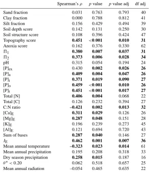
Table 1. Spearman’sρfor relationships between above-ground coarse wood production and a range of soil and climate predictors. Probabil-ities (p) are given with and without adjustment (adj) for degrees of freedom (df) according to Dutillieul (1993). Abbreviations used:51and
52– first and second indices of soil physical conditions (Sect. 2.2);[P]ex,[P]a,[P]i,[P]o,[P]t– extractable, available, inorganic, organic, and total soil phosphorus pools;[Ca]E,[Mg]E,[K]E,[Al]E- exchangeable calcium, magnesium, potassium and aluminium concentrations;
IE- effective soil cation exchange capacity;θ∗<0.20 – modelled number of months with soil water less than 0.2 of maximum available soil water content. Wherep≤0.050 values are shown in bold.
Spearman’sρ pvalue pvalue adj df adj
Sand fraction 0.031 0.763 0.793 40
Clay fraction 0.000 0.788 0.812 41
Silt fraction 0.156 0.429 0.494 39
Soil depth score 0.142 0.131 0.250 30
Soil structure score 0.108 0.396 0.424 47
Topography score 0.451 <0.001 0.010 31
Anoxia score 0.162 0.376 0.330 62
51 0.380 0.007 0.037 31
52 0.373 0.006 0.028 34
pH 0.315 0.054 0.194 24
[P]ex 0.430 0.002 0.026 26
[P]a 0.409 0.004 0.047 26
[P]i 0.371 0.019 0.090 27
[P]o 0.459 <0.001 0.010 26
[P]t 0.451 <0.001 0.017 27
Total [N] 0.406 0.004 0.068 22
Total [C] 0.126 0.232 0.394 27
C:N ratio –0.421 0.002 0.013 32
[Ca]E 0.311 0.029 0.126 26
[Mg]E 0.287 0.048 0.151 28
[K]E 0.196 0.239 0.273 45
[Al]E 0.121 0.694 0.720 43
Sum of bases 0.287 0.040 0.146 27
IE 0.462 0.001 0.007 36
Mean annual temperature –0.323 0.023 0.014 61
Mean annual precipitation 0.195 0.208 0.318 33
Dry season precipitation 0.258 0.015 0.187 16
θ∗<0.20 0.062 0.518 0.657 25
Mean annual radiation –0.054 0.465 0.635 22
3.2 Underlying causes of variation
An understanding of biomass, productivity and turnover vari-ation across a large area such as the Amazon Basin (Fig. 1) requires some knowledge of the “internal components” giv-ing rise to the stand-to-stand variation. For example, a Basin-wide gradient inϕ(which is expressed here as a proportion of the total tree population) could arise (in one extreme) from the same number of trees entering/leaving the population per unit area per year, but variable stand densities (S). Or (in the other extreme) it could arise from an invariantS and a variable number of trees entering/leaving the population per unit area per year. Similarly, stand-to-stand variations inWP could be due to differences in average individual tree growth rates and/or differentS. Likewise different stand biomasses (B) can potentially arise through any combination of vari-ability inS, basal area per tree (At) and wood density (%w) with significant covariances also possible.
0.00 2.00 4.00 6.00 8.00 10.00 12.00
W
P
(M
g
h
a
yr
)
-1
-1
4 8 16 32 64 128
Readily available P (mg kg )-1
10 100 1,000
Total extractable P (mg kg )-1
4 8 16 32 64 128 256 512
Total organic P (mg kg )-1
0.00 2.00 4.00 6.00 8.00 10.00 12.00
WP
(M
g
h
a
yr
)
-1
-1
10 100 1,000
Total P (mg kg )-1
0.01 0.10 1.00 10.00
Exchangeable Ca (cmol kg )c -1
0.02 0.05 0.14 0.37 1.00 2.72
Exchangeable Mg (cmol kg )c -1
0.00 2.00 4.00 6.00 8.00 10.00 12.00
W
P
(M
g
h
a
yr
)
-1
-1
0.02 0.05 0.14 0.37
Exchangeable K (cmol kg )c -1
0.1 1.0 10.0
Sum of bases (cmol kg )c -1
0.01 0.10 1.00
Nitrogen (%)
Arenosols Podzols
Ferralsols Acrisols
Lixisols Nitisols
Plinthosols Alisols
Umbrisols Cambisols
Fluvisols Gleysols
Leptosols
Fig. 3. Relationships between above-ground coarse wood production (WP) and different soil nutrient measures.
3.3 Coarse wood production
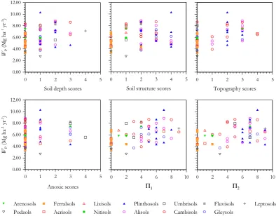
Spatially adjusted Spearman’sρdescribing the relationships betweenWP and the studied edaphic and climatic variables are shown in Table 1. Of the soil chemistry predictors, the best associations ofWPwere with the various pools of phos-phorus, with ρ decreasing from 0.46 to 0.37 in the order [P]o>[P]t>[P]ex>[P]a>[P]i. All correlations remained significant after adjustment of degrees of freedom for spatial autocorrelation (Table 1). Soil nitrogen was positively corre-lated and soil C:N ratio negatively correcorre-lated toWP, with soil exchangeable cations and6B also of a limited positive in-fluence. Effective cation exchange capacity was also
0.00 2.00 4.00 6.00 8.00 10.00 12.00
W
P
(M
g
h
a
yr
)
-1
-1
0 1 2 3 4 5
Soil depth scores
Arenosols Podzols
Ferralsols Acrisols
Lixisols Nitisols
Plinthosols Alisols
Umbrisols Cambisols
Fluvisols Gleysols
Leptosols
0 1 2 3 4 5
Soil structure scores
0 1 2 3 4 5
Topography scores
0.00 2.00 4.00 6.00 8.00 10.00 12.00
W
P
(M
g
h
a
yr
)
-1
-1
0 1 2 3 4 5
Anoxic scores
0 2 4 6 8 10 0 2 4 6 8 10
[image:11.595.99.494.64.372.2]Π1 Π2
Fig. 4. Relationships between above-ground coarse wood production (WP) and soil physical properties. For definitions of51and52see Sect. 2.2.
Of the climate variables,TAshowed only a relatively weak negative correlation withWP, and with dry–season precip-itation,PD, showing a more consistent positive relationship than that observed for mean annual precipitation,PA(Fig. 5); this is also evidenced by its higher Spearman’sρ. Neverthe-less, neither of these measures were significant atp≤0.10 after an adjustment for the relevant degrees of freedom (Ta-ble 1). Nor was there an indication of a role for mean annual radiation variations across the Basin as an important mod-ulator ofWP, although we do also note that the fidelity of the radiation estimates used remains largely unknown for our study area.
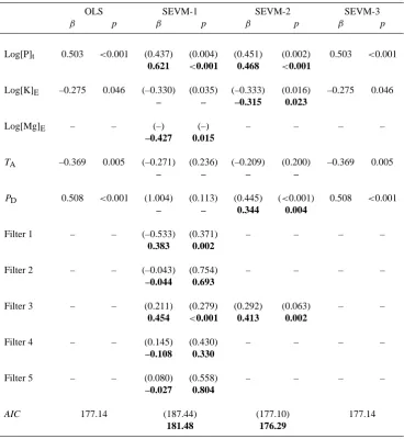
Results of multiple regression analysis, with and without the inclusion of spatial filters are given in Table 2. All of [K]E,[P]t,TAandPDwere selected in the lowestAI COLS model (R2=0.46) and with all four variables significant at p <0.05. The model selected with the lowest AI C crite-rion but with all spatial filters with a Moran’sI >0.1 in-cluded (i.e. SEVM-01) was, however, substantially different. Although [P]t remained as a strong predictor term, [Mg]E replaced [K]Eas the (negatively affecting) influential cation and with temperature and precipitation terms not selected (R2=0.48). For SEVM-02, where there was a solitary filter selected on the basis of a prior correlation withWP, then the
results were more similar to the OLS case, but with, as for SEVM-01, TA excluded (R2=0.46). For SEVM-03, there was no spatial filter found to be significantly correlated with the OLS model residuals. Thus the model presented is simply the OLS case.
Also shown in Table 2 are (in brackets) the model fits for the variables selected by the minimum AI C OLS models, but with the SEVM-01 or SEVM-02 filters also included. In most cases, the standardised coefficients (β) and their level of significance were reduced in the presence of spatial fil-ters and with these reductions being greatest for SEVM-01 (which has the more liberal spatial filter selection criteria). One notable exception to this pattern was PD which had a greatly increased value in SEVM-01 as compared to the OLS/SEVM-03 and SEVM-02 models.
0.00 2.00 4.00 6.00 8.00 10.00 12.00
WP
(M
g
h
a
yr
)
-1
-1
23 24 25 26 27 28
Mean annual temprerature ( C)o
Arenosols Podzols Ferralsols
Acrisols Lixisols Nitisols
Plinthosols Alisols Umbrisols
Cambisols Fluvisols Gleysols
Leptosols 1,000 2,000 3,000 4,000 5,000
Mean annual precipitation (mm)
0.00 2.00 4.00 6.00 8.00 10.00 12.00
W
P
(M
g
h
a
yr
)
-1
-1
Average dry season precipitation (mm month )-1
0 1 2 3 4 5
# months <20% AWC
[image:12.595.159.437.61.377.2]0 100 200 300
Fig. 5. Relationships between above-ground coarse wood production (WP) and climatic factors.
predictor ofWPthan any other soil phosphorus pool; this be-ing both in terms of the number of models with1AI C <2.0 for which it was a component and in terms of having much higher standardised coefficients. A similar result was found forPDwhich was a much more frequently selected predictor ofWPthan wasPA.
As shown in the Supplement (Eq. S5),WPcan be consid-ered (to good approximation) as the product of basal area growth rate (GB) and%w. An analysis of soil and climate ef-fects on the latter is presented in the next section and with a similar analysis forGBprovided in the Supplement. ForGB we found our selection procedure to imply similar climatic and edaphic factors as the best predictors forWP; this being the case both with and without the inclusion of spatial fil-ters. Specifically, the OLS regression results indicate a role of [P]T,TAandPAbut with a less significant52term also se-lected (Supplement, Table S2). Interestingly, although mean annual radiation (Ra) did not appear as a significant predictor forWP, it turns out to be significant atp=0.004 forGBin the model selection undertaken with SEVM-2 spatial filters but not for the OLS or other SEVM models. Also of note is the absence of any apparent influence of cations onGB. This contrasts with the negative effect of one of [K]Eor [Mg]Eon WPas suggested by the multivariate regression results (Table 2).
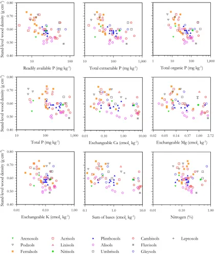
3.4 Wood density
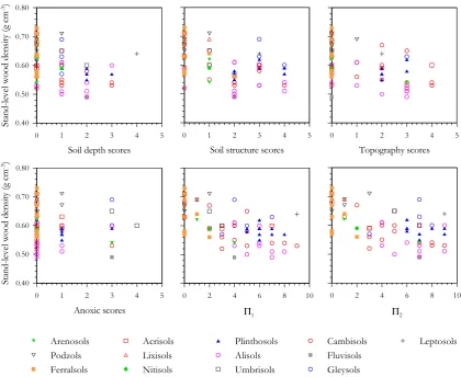
Spearman’sρ with and without probability values and de-grees of freedom adjusted for spatial autocorrelation are listed for relationships between measured edaphic and cli-matic variables and plot-level%w in Table 3. This shows%w to have negative associations with many soil nutrient char-acteristics and physical properties, as well as with climatic variables such asTA,PA andPD. Relationships are shown further for edaphic predictors in Fig. 6 (soil chemistry) and Fig. 7 (soil physical properties). All soil phosphorus pools and base cation measures showed negative relationships with %w and with most soil physical properties also strongly re-lated. Specifically, soil depth, soil structure and topogra-phy were all negatively correlated, but with anoxic condi-tions showing no clear relacondi-tionship. The combined indexes of physical properties also had strong negative relationships with%w, with51the most strongly correlated (ρ=−0.66).
Table 2. LowestAI Cmodel fits for the prediction of coarse wood productivity with and without the use of spatial filters. For each variable, the upper line gives first the standardised coefficients (β) and their level of significance (p) from the best OLS model fit followed by (in brackets) the results when the same OLS model is applied with the preselected spatial filter included. Also shown in bold (second line) for each variable are the values ofβand p obtained for the lowest AIC model fit with the spatial filters included. Variables not included in any given model fit are denoted with a “–”. Variables: [P]t; total soil phosphorus: [K]E; exchangeable soil potassium: [Mg]E; exchangeable soil magnesium:TA; mean annual air temperature:PD; dry season precipitation. The numbering of the spatial filters is inconsequential.
OLS SEVM-1 SEVM-2 SEVM-3
β p β p β p β p
Log[P]t 0.503 <0.001 (0.437) (0.004) (0.451) (0.002) 0.503 <0.001 0.621 <0.001 0.468 <0.001
Log[K]E –0.275 0.046 (–0.330) (0.035) (–0.333) (0.016) –0.275 0.046
– – –0.315 0.023
Log[Mg]E – – (–) (–) – – – –
–0.427 0.015
TA –0.369 0.005 (–0.271) (0.236) (–0.209) (0.200) –0.369 0.005
– – – –
PD 0.508 <0.001 (1.004) (0.113) (0.445) (<0.001) 0.508 <0.001
– – 0.344 0.004
Filter 1 – – (–0.533) (0.371) – – – –
0.383 0.002
Filter 2 – – (–0.043) (0.754) – – – –
–0.044 0.693
Filter 3 – – (0.211) (0.279) (0.292) (0.063) – –
0.454 <0.001 0.413 0.002
Filter 4 – – (0.145) (0.430) – – – –
–0.108 0.330
Filter 5 – – (0.080) (0.558) – – – –
–0.027 0.804
AIC 177.14 (187.44) (177.10) 177.14
181.48 176.29
The best OLS regression fit (Table 4) was for a model hav-ing51, [K]EandTA as predictors, with this model yielding anR2of 0.59. Within this model, theTAand51effects were highly significant (p=0.002 and p <0.001, respectively), but with the negative [K]Eeffect much less so (p=0.12).
In contrast to WP, inclusion of spatial filters through SEVM-01 or SEVM-02 resulted in different soil and climate variables being selected by the minimumAI Ccriterion, with [K]Ereplaced by [Mg]EandTAreplaced byPDin both these models. Plant available phosphorus ([P]a: see Sect. 2.2) was also selected in the lowestAI C SEVM-01 model and with this model also not including51.
Two of the eight potential eigenvector filters were corre-lated with the OLS model residuals and, when added to the OLS regression model to give SEVM-3, these caused some change to the OLS result. Although theTAand51effects did not show large changes in significance levels (p=0.004 and p≤0.001, respectively), for [K]Ethis was much reduced at onlyp=0.61. The effect of adding these spatial filters was much less than for those added through the SEVM-01 and SEVM-02 procedures for whichTAended up being the only environmental term selected by both models, and with51 still significant in SEVM-02.
Table 3. Spearman’sρfor relationships between stand-level wood density and a range of soil and climate predictors. Probabilities (p) are given with and without adjustment (adj) for degrees of freedom (df) according to Dutillieul (1993). Abbreviations used:51and52– first and second indices of soil physical conditions (Sect. 2.2);[P]ex,[P]a,[P]i,[P]o,[P]t– extractable, available, inorganic, organic and total soil phosphorus pools;[Ca]E,[Mg]E,[K]E,[Al]E- exchangeable calcium, magnesium, potassium and aluminium concentrations;IE– effective soil cation exchange capacity;θ∗<0.20 – modelled number of months with soil water less than 0.2 of maximum available soil water content. Wherep≤0.050 values are shown in bold.
Variable Spearman’sρ pvalue pvalue adj df adj
Sand fraction 0.069 0.536 0.520 55
Clay fraction 0.038 0.125 0.058 78
Silt fraction −0.430 <0.001 0.064 16
Soil depth score −0.450 <0.001 0.040 17
Soil structure score −0.523 <0.001 0.052 11
Topography score −0.520 <0.001 0.121 10
Anoxia −0.142 0.265 0.337 38
51 −0.662 <0.001 0.036 8
52 −0.542 <0.001 0.045 7
pH −0.333 0.057 0.071 45
[P]ex −0.552 0.007 0.104 19
[P]a −0.538 <0.001 0.076 16
[P]i −0.497 0.008 0.073 24
[P]o −0.535 0.014 0.140 19
[P]t −0.470 <0.001 0.031 20
Total [N] −0.330 0.263 0.436 25
Total [C] 0.019 0.680 0.766 27
C:N ratio 0.633 <0.001 0.025 9
[Ca]E −0.518 <0.001 0.026 21
[Mg]E −0.551 <0.001 0.019 22
[K]E −0.457 <0.001 0.041 17
[Al]E 0.086 0.987 0.990 31
Sum of bases −0.552 <0.001 0.022 21
IE −0.489 <0.001 0.048 14
Mean annual temperature 0.499 <0.001 0.007 26
Mean annual precipitation −0.257 0.006 0.296 8
Dry season precipitation −0.300 <0.001 0.304 5
θ∗<0.20 –0.167 0.828 0.928 9
Mean annual radiation –0.007 0.762 0.871 17
(data not shown), suggesting that both measures of soil phys-ical properties were equally good predictors of stand level wood density variations. Indeed, for the seven valid OLS models with1AI C≤2, all included51. All these models also includedTAwith six of these models also including one or more exchangeable cations. Phosphorus and precipitation measures on the other hand were not selected in any OLS model with an1AI C≤2. Examining models in SEVM-1 and SEVM-2 with1AI C≤2, we found that some measure of precipitation and51were present in most models. Only SEVM-1 models included a phosphorus term, whilst at least one soil cation term was present in all models and with [Mg]E selected in most models.
We can have some confidence in soil physical conditions having an important role in the modulation of stand level wood density as51was found to be a significant predictor in most cases with a high level of statistical significance. The roles for temperature and precipitation are, however, much
more ambiguous. Although there is some suggestion for trees with lower wood densities associating with soils of a higher cation status, it is not clear through which cation(s) this effect is mediated.
3.5 Stem turnover rates
10 100 1,000
Total extractable P (mg kg )-1
0.40 0.50 0.60 0.70 0.80
S
ta
n
d
-l
ev
el
w
o
o
d
d
en
si
ty
(g
cm
-3)
10 100
Readily available P (mg kg-1)
1 10 100 1,000
Total organic P (mg kg )-1
0.40 0.50 0.60 0.70 0.80
10 100 1,000
Total P (mg kg )-1
0.01 0.10 1.00 10.00
Exchangeable Ca (cmol kg )c -1
Arenosols Podzols Ferralsols
Acrisols Lixisols Nitisols
Plinthosols Alisols Umbrisols
Cambisols Fluvisols Gleysols
Leptosols
0.02 0.05 0.14 0.37 1.00 2.72
Exchangeable Mg (cmol kg )c -1
0.40 0.50 0.60 0.70 0.80
0.01 0.10 1.00
Exchangeable K (cmol kg )c -1
0.1 1.0 10.0
Sum of bases (cmol kg )c -1
0.01 0.10 1.00
Nitrogen (%)
St
an
d
-l
ev
el
w
o
o
d
d
en
si
ty
(g
cm
-3)
S
ta
n
d
-l
ev
el
w
o
o
d
d
en
si
ty
(g
cm
-3)
Fig. 6. Relationships between average stand wood density and different soil nutrient measures.
rate (Fig. 9) confirm that Amazon forest stand dynamics are well correlated with many measures of soil nutrient status.
Individual soil physical property scores were also associ-ated with variations inϕ, with soil structure and soil depth having the highestρ. Relationships are shown in Fig. 10. Soil depth, structure and topography show some relationship with tree turnover rates but with no clear pattern evident for soil anoxic conditions. Both indexes of soil physical properties were also strongly related to tree turnover rates. Climatic
pre-dictors on their own were, however, only loosely associated with variations inϕ(Fig. 11).
[image:15.595.88.511.65.563.2]0.40 0.50 0.60 0.70 0.80
S
ta
n
d
-l
ev
el
w
o
o
d
d
en
si
ty
(g
cm
)
-3
0 1 2 3 4 5
Soil depth scores
Arenosols Podzols Ferralsols
Acrisols Lixisols Nitisols
Plinthosols Alisols Umbrisols
Cambisols Fluvisols Gleysols
Leptosols
0 1 2 3 4 5
Soil structure scores
0 1 2 3 4 5
Topography scores
0.40 0.50 0.60 0.70 0.80
0 1 2 3 4 5
Anoxic scores
0 2 4 6 8 10
Π1
0 2 4 6 8 10
Π2
S
ta
n
d
-l
ev
el
w
o
o
d
d
en
si
ty
(g
cm
)
-3
Fig. 7. Relationships between wood density and soil physical properties.For definitions of51and52see Sect. 2.2.
selection of one of51or52in both models. A negative ef-fect of dry season precipitation of stand–level turnover rates was also suggested through the selection ofPDin SEVM-02. When the SEVM-01 and SEVM-02 filters were added to the OLS model, only51 retained significance atp <0.05. This drastic response contrasted with the SEVM-03 proce-dure where the standardised coefficients and their levels of significance were only slightly reduced for both52andPA. There was, however, a much more substantial reduction in apparent significance for6Bin SEVM-03 (p=0.210).
Examining the 28 alternative OLS models with1AI C≤ 2.0, all models had either51or52 as a significant predic-tor along with one significant precipitation measure (either PA orPD) and a measure of soil cations and/or phosphorus as alternative or additional predictors (13 models had some measure of cations included, while some form of phosphorus was present in 10 models). Likewise for potentially alterna-tive models under SEVM-02, one of51or52was always present. Taken together, these results suggest an unequivocal role of soil physical properties in driving tree turnover rates in Amazonia, but with amount and distribution of precipita-tion also important.
3.6 Stand biomass
Spearman’sρwith and withoutpvalues and degrees of free-dom adjusted for spatial autocorrelation are listed forB in Table 7. Forest biomass was generally negatively correlated to both soil cation and phosphorus measurements (Fig. 12), with the best correlations amongst the soil chemistry param-eters being the various soil phosphorus pools, which varied fromρ=−0.48 toρ=−0.28. Exchangeable cations also had negative correlations with B, with [K]E and [Mg]E show-ing the stronger relationships (ρ = −0.45 and ρ = −0.31 respectively). Correlations with both soil phosphorus pools and exchangeable cations remained significantp≤0.05 af-ter correction for spatial autocorrelation.
[image:16.595.87.508.65.409.2]0.40 0.50 0.60 0.70 0.80
St
an
d
-l
ev
el
w
o
o
d
d
en
si
ty
(g
cm
)
-3
23 24 25 26 27 28
Mean annual temperature ( C)o
Arenosols Podzols Ferralsols
Acrisols Lixisols Nitisols
Plinthosols Alisols Umbrisols
Cambisols Fluvisols Gleysols
Leptosols
1,000 2,000 3,000 4,000 5,000
Mean annual precipitation (mm)
0.40 0.50 0.60 0.70 0.80
St
an
d
-l
ev
el
w
o
o
d
d
en
si
ty
(g
cm
)
-3
0 100 200 300
Average dry season precipitation (mm month )-1
0 1 2 3 4 5
# months <20% AWC
Fig. 8. Relationships between stand wood density and climatic factors.
physical properties andBremained marginally significant af-ter spatial correction (p≤0.10) with the exception of topog-raphy and51(p >0.15: Table 7).
Above-ground biomass was also positively correlated with TA,PA andPD and strongly negatively correlated with the number of months for which θ∗<0.2. These relationships betweenB and climatic variables are shown in Fig. 14. This suggests some response to rainfall amount as well as to its distribution during the dry season.
The results for multiple regression models with and with-out the addition of spatial filters are given in Table 8. The best OLS model retained [P]t, [K]E,PDand52as predictors for B, with an overallR2of 0.38. Of note is the change in sign for [P]t with a positive relationship withBbeing suggested by the multivariate model as compared to a negative (albeit non-significant) association withB when considered on its own (Table 7, Table 8, Fig. 12).
The selection of filters through the SEVM-1 and SEVM-2 procedures resulted in two filters selected by SEVM-1 and three filters selected by SEVM-2.When the SEVM-01 filters were applied, the lowestAI C model (R2=0.65) included only [Ca]E and with none of the OLS variables selected. Only [K]Ewas included in the lowestAI CSEVM-02 model
(R2=0.53). Consistent with the large effects of the filters in these models, none of the OLS-selected variables remained significant when the filters from either 01 or SEVM-02 were included in a new model fit.
Regression with the two filters selected by the SEVM-3 procedure had varying effects on the levels of significance of the OLS predictors. Although total soil phosphorus had its significance level improved from p=0.02 to p <0.01 andPD had no significant change, [K]Ehad its significance level reduced fromp=0.003 top=0.023 and with52also being much less significant after filter addition (p=0.106). The inclusion of these two filters improved the overall model fit substantially with anR2=0.51 as compared to 0.38 for the OLS fit.
Only three alternative OLS models with1AI C≤2 were found; these being very similar to the best model, but with the difference of [Ca]E appearing in addition to [K]E in the second lowestAI C model andTAappearing in addition to PDin the third model.
Table 4. LowestAI Cmodel fits for the prediction of stand wood density with and without the use of spatial filters. For each variable, the upper line gives first the standardised coefficients (β) and their level of significance (p) from the best OLS model fit, followed by the results (in brackets) when the same OLS model is applied with the preselected spatial filter included. Also shown in bold (second line) for each variable are the values ofβand p obtained for the lowest AIC model fit with the spatial filters included. Variables not included in any given model fit are denoted with a “–”. Variables:51; Quesada et al (2010)’s first index of soil physical properties; [P]a; readily available soil phosphorus: [K]E; exchangeable soil potassium: [Mg]E; exchangeable soil magnesium: [P]a; plant available phosphorus:TA; mean annual air temperature:PD; dry season precipitation. The numbering of the spatial filters is inconsequential.
OLS SEVM-1 SEVM-2 SEVM-3
β p β p β p β p
51 –0.495 <0.001 (–0.167) (0.295) (–0.291) (0.036) –0.496 <0.001
– – -0.257 0.030
Log[K]E –0.175 0.121 (–0.063) (0.561) (–0.062) (0.567) –0.054 0.611
– – – –
Log[Mg]E – – (–) (–) (–) (–) – –
–0.330 <0.001 –0.223 0.011
Log[P]a – – (–) (–) – –
0.201 0.093 –
TA 0.321 0.002 (0.211) (0.048) (0.260) (0.005) 0.270 0.004
– – – –
PD – – (–) (–) (–) (–) – –
–0.828 <0.001 –0.654 <0.001
Filter 1 – – (0.248) (0.039) (0.172) (0.127) – –
–0.378 0.084 –0.399 0.023
Filter 2 – – (–0.210) (0.028) – – – –
–0.270 <0.001
Filter 3 – – (0.441) (<0.001) (0.377) (<0.001) 0.296 0.005 0.703 <0.001 0.506 <0.001
Filter 4 – – (0.139) (0.110) – – – –
0.103 0.230
Filter 5 – – (0.011) (0.900) – – – –
0.080 0.247
Filter 6 – – (–0.079) (0.365) – – – –
0.117 0.235
Filter 7 – – (0.211) (0.120) (0.185) (0.035) – –
0.173 0.035 0.136 0.097
Filter 8 – – (0.096) (0.256) – – 0.173 0.049
–0.012 0.867
AIC –177.667 (–183.31) (–186.169) –186.405
[image:18.595.111.485.168.695.2]Table 5. Spearman’sρfor relationships between stand-level turnover rates and a range of soil and climate predictors. Probabilities (p) are given with and without adjustment (adj) for degrees of freedom (df) according to Dutillieul (1993). Abbreviations used:51and52– first and second indices of soil physical conditions (Sect. 2.2);[P]ex,[P]a,[P]i,[P]o,[P]t– extractable, available, inorganic, organic and total soil phosphorus pools;[Ca]E,[Mg]E,[K]E,[Al]E- exchangeable calcium, magnesium, potassium, and aluminium concentrations;IE– effective soil cation exchange capacity;θ∗<0.20 – modelled number of months with soil water less than 0.2 of maximum available soil water content. Wherep≤0.050 values are shown in bold.
Variable Spearman’sρ pvalue pvalue adj df adj
Sand fraction –0.141 0.243 0.250 52
Clay fraction 0.095 0.876 0.885 46
Silt fraction 0.272 0.034 0.064 41
Soil depth score 0.381 0.001 0.008 35
Soil structure score 0.526 <0.001 0.002 29
Topography score 0.311 0.040 0.125 30
Anoxia score 0.183 0.082 0.089 52
51 0.527 <0.001 0.002 25
52 0.554 <0.001 0.001 25
pH 0.332 0.004 0.022 35
[P]ex 0.559 <0.001 0.002 27
[P]a 0.561 <0.001 0.003 26
[P]i 0.469 <0.001 0.009 29
[P]o 0.568 <0.001 0.001 27
[P]t 0.489 <0.001 0.001 33
Total [N] 0.252 0.051 0.119 35
Total [C] –0.077 0.880 0.899 39
C:N ratio −0.570 <0.001 <0.001 33
[Ca]E 0.336 <0.001 0.003 41
[Mg]E 0.449 <0.001 0.001 40
[K]E 0.442 <0.001 0.009 32
[Al]E 0.036 0.812 0.828 45
Sum of bases 0.368 <0.001 0.002 39
IE 0.587 <0.001 <0.001 42
Mean annual temperature –0.145 0.101 0.179 36
Mean annual precipitation –0.06 0.626 0.773 19
Dry season precipitation –0.046 0.915 0.956 15
θ∗<0.20 0.265 0.027 0.189 19
Mean annual radiation 0.128 0.792 0.855 26
that although there is some variability in%w, it is differences inABthat to a large extent drive the variations inB, except at very high values. Similar analyses to those done forB here,
viz. an examination of driving variables with and without
spa-tial autocorrelation issues, is therefore also given forAB in Table S2. This shows similar results to have been attained for ABas was the case forB, especially for the OLS and SEVM-03 models.
3.7 Partitioning of environmental versus spatial components of variation
Figure 15 shows the partitioning of the variation inWP,%w, ϕandB as Venn diagrams. Only in the case ofWPwas the environmental component (a) greater than the shared compo-nent (b) and in all cases this shared compocompo-nent was greater than that attributable solely to the spatial component (c). No-tably small fractions of the variation were attributable solely
0.00 1.00 2.00 3.00 4.00 5.00
St
an
d
-l
ev
el
tr
ee
tu
rn
o
ve
r
ra
te
(%
yr
)
-1
4 8 16 32 64 128
Readily available P (mg kg )-1
0.03 0.06 0.13 0.25 0.50 1.00
Nitrogen (%) 0.01 0.10 1.00 10.00
Exchangeable Ca (cmol kg )c -1
Arenosols Podzols
Ferralsols Acrisols
Lixisols Nitisols
Plinthosols Alisols
Umbrisols Cambisols
Fluvisols Gleysols
Leptosols 0.02 0.05 0.14 0.37 1.00 2.72
Exchangeable Mg (cmolckg ) -1
0.1 1.0 10.0
Sum of bases (cmol kg )c -1
10 100 1,000
Total extractable P (mg kg )-1
1 10 100 1,000
Total organic P (mg kg )-1
0.00 1.00 2.00 3.00 4.00 5.00
10 100 1,000
Total P (mg kg )-1
0.00 1.00 2.00 3.00 4.00 5.00
0.02 0.05 0.14 0.37
Exchangeable K (cmol kg )c -1
St
an
d
-l
ev
el
tr
ee
tu
rn
o
ve
r
ra
te
(%
yr
)
-1
St
an
d
-l
ev
el
tr
ee
tu
rn
o
ve
r
ra
te
(%
yr
)
-1
Fig. 9. Relationships between tree turnover rates and different soil fertility parameters.
4 Discussion
4.1 Spatial structures and spatial autocorrelation
Implied roles for the examined climatic and edaphic predic-tors in modulating Amazon forest structure and dynamics de-pended to a large degree on the assumptions made as to the causes for the strong spatial patterning in response variables observed. Complicating this matter, effects of spatial filter inclusion were not predictable, with the magnitude of model differences in terms of variables selected, changes in values of standardised coefficients, and associated levels of
[image:20.595.102.498.65.529.2]0.00 1.00 2.00 3.00 4.00 5.00
S
ta
n
d
-l
ev
el
tr
ee
tu
rn
o
v
er
ra
te
s
(%
yr
)
-1
0 1 2 3 4 5
Soil depth scores
Arenosols Podzols
Ferralsols Acrisols
Lixisols Nitisols
Plinthosols Alisols
Umbrisols Cambisols
Fluvisols Gleysols
Leptosols
0 1 2 3 4 5
Soil Structure scores
0 1 2 3 4 5
Topography scores
0.00 1.00 2.00 3.00 4.00 5.00
0 1 2 3 4 5
Anoxic scores
0 2 4 6 8 10
Π1
0 2 4 6 8 10
Π2
S
ta
n
d
-l
ev
el
tr
ee
tu
rn
o
v
er
ra
te
s
(%
yr
)
-1
Fig. 10. Relationships between tree turnover rates and soil physical properties. For definitions of51and52see Sect. 2.2.
As a variant of this, the SEVM-03 approach is roughly com-parable to the criterion adopted by Griffith and Peres-Neto (2006) where only eigenvectors that minimise Moran’sI in regression residuals are included (Bini et al., 2009). This ef-fectively then assumes that all spatial structures in the dataset which are not correlated with model residuals must be caused by the predictor variables.
On the other hand, model selections through SEVM-01 and SEVM-02 represent an approach where unidentified spa-tial processes are considered an alternative explanation for the observed geographical variations in stand properties. In the case of SEVM-01, with filters first selected on the basis of their Moran’sIand then put forward for selection in a model also including environmental variables, then as pointed out by Diniz-Filho et al. (2008) a fundamental tautology exists. This is because the dependent variable has already been used to select the independent variable against which it is subse-quently tested. It could be argued therefore, that SEVM-01 effectively involves a null hypothesis that all observed vari-ation in the response variable can be accounted for through endogenous spatial processes alone and that none of it is re-lated to the studied climatic and edaphic variables.
This is not necessarily a nonsense proposition. For exam-ple, many physiological and structural traits related to Ama-zon forest growth and mortality have strong phylogenetic associations (Baker et al., 2004a; Fyllas et al., 2009, 2012;
[image:21.595.107.490.63.353.2]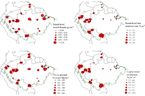


![Table 4.E; exchangeable soil potassium: [Mg]air temperature: PD) and their level of significance (pmodel fit are denoted with a “–”](https://thumb-us.123doks.com/thumbv2/123dok_us/162569.39713/18.595.111.485.168.695/table-exchangeable-potassium-temperature-level-signicance-pmodel-denoted.webp)