Analytic approximations for computing probit choice probabilities

promoting access to White Rose research papers

White Rose Research Online [email protected]

Universities of Leeds, Sheffield and York

http://eprints.whiterose.ac.uk/

This is an author produced version of a paper published in Transportmetrica. White Rose Research Online URL for this paper:

http://eprints.whiterose.ac.uk/77195/

Paper:

Connors, RD, Hess, S and Daly, A (2012) Analytic approximations for computing probit choice probabilities. Transportmetrica, 10 (2). 119 – 139.

Page 1 Title: Analytic Approximations for Computing Probit Choice Probabilities

Authors: Dr Richard D. Connors [corresponding author]

Institute for Transport Studies, University of Leeds, Leeds, LS2 9JT, United Kingdom Tel: +44 113 3431799

Fax: +44 113 3435334

Email: [email protected] Dr Stephane Hess

Institute for Transport Studies, University of Leeds, Leeds, LS2 9JT, United Kingdom Tel: +44 113 3436611

Fax: +44 113 3435334

Email: [email protected] Prof Andrew Daly

Institute for Transport Studies, University of Leeds, Leeds, LS2 9JT, United Kingdom and RAND Europe, Westbrook Centre, Milton Road, Cambridge, CB4 1YG, United Kingdom Tel: +44 1223 353 329

Page 2 Abstract

The multinomial probit model has long been used in transport applications; as the basis for mode- and route-choice in computing network flows, and in other route-choice contexts when estimating preference parameters. It is well known that computation of the probit choice probabilities presents a significant computational burden, since they are based on multivariate normal integrals. Various methods exist for computing these choice probabilities, though standard Monte Carlo is most commonly used. In this paper we compare two analytical approximation methods (Mendell-Elston and Solow-Joe) with three Monte Carlo approaches for computing probit choice probabilities. We systematically investigate a wide range of parameter settings and report on the accuracy and computational efficiency of each method. The findings suggest that the accuracy and efficiency of the optimal Mendell-Elston analytic approximation method offers great potential for wider use.

Keywords

Multinomial Probit, Multivariate Normal Integral, Analytical Approximation, Choice Probabilities

1. Introduction

The random utility paradigm models choice by identifying the chosen alternative as the one with the highest utility. With the recognition that only part of this utility can be modelled deterministically, a key assumption made in estimation as well as application of such models concerns the distribution used to represent the remaining random part of utility. This assumption has major implications in terms of the ability to represent core phenomena such as unexplained taste heterogeneity across respondents and across choices for the same respondent, correlation across choices for the same respondent, and heteroskedasticity across respondents and/or alternatives. Crucially, it also has major implications in terms of the computational cost of both model estimation and application. The choice probabilities are given by multivariate integrals over the distribution of the error terms, and these multivariate integrals only have a closed form solution for certain choices of distribution, such the family of GEV models (McFadden, 1978a, and also see overview in Train, 2009).

While the standard closed form GEV models are appealing due to their low computational cost in estimation and application, there are limits to the degree of complexity that can be conveniently represented by making use only of (generalised) extreme value distributions for the error term. This justifies moving away from such assumptions in certain contexts. The case where the error terms have a joint multivariate normal (MVN) distribution is referred to as the (multinomial) probit model (dating back to Thurstone, 1927). Network modellers in particular use the probit specification across a host of application areas, for example for modelling demand (Zito et al 2010), parking (Teng et al. 2008), accidents (Rifaat & Chin 2007), route and mode choice (Connors et al. 2007, Sumalee et al. 2009). Similarly, the choice modelling community is well aware of the theoretical appeal of the probit structure, allowing them to address the various core behavioural phenomena highlighted above. Nevertheless, in the particular context of choice modelling, interest in the probit model waned with the increasing use mixed logit (see e.g. Train, 2009, Dalal & Klein, 1988, McFadden & Train, 2000), which has a number of advantages in terms of distributional assumptions and ease of estimation. However, the error structure of the probit model remains appealing, and interest in the error structure of the probit model has been reinvigorated by Bhat’s recent work (Bhat, 2010; Bhat and Sidharthan, 2010; Bhat et al., 2010) that highlights the benefit of adopting the probit choice model within a composite marginal likelihood (CML) framework for the estimation of choice preferences based on survey data1.

Notwithstanding identification issues arising from the number of parameters that may need to be estimated (Dansie, 1985; Bunch, 1991; Keane, 1992), the key constraint in using the probit model remains the cost of

1

Page 3

computing the choice probabilities that do not have a closed form expression. This is an issue for both prediction and model estimation, where there is a need to evaluate the choice probabilities efficiently and accurately. Numerical integration methods have been developed to accurately compute MVN integrals (see Drezner and Wesolowsky, 1990; Genz, 1992, 2004; Drezner, 1994; Genz and Bretz, 1999, 2002); indeed methods based on these approaches are implemented in commercial software (e.g. MATLAB) offering off-the-shelf accuracy of at least for each choice probability in choice sets having up to 25 alternatives. However, the execution time for these methods increases very rapidly with both the problem dimension and the accuracy demanded from them. For practical applications that require calculation of very many choice probabilities, these methods are not fast enough.

The standard approach seen in most applications is to evaluate probit choice probabilities via simple frequency simulation (Manski and Lerman, 1981): the utilities of the alternatives are drawn from their distribution, the alternative with the highest utility is chosen. This is repeated a number of times, and the choice probability of each alternative is approximated by its choice frequency. This approach faces several difficulties: capturing low probability alternatives; the results depend on the seed used for the random number generator (i.e. ‘noise’ is present); and the frequencies are not continuous. The last issue was tackled by McFadden (1989) who processed the simulated frequencies via a logit function. Possibly the most sophisticated simulation-based approach is the GHK probability simulator (see Börsch-Supan and Hajivassiliou, 1993). This approach rewrites the MVN integral as a product of marginal conditional probabilities, and evaluates these marginal probabilities in turn by Monte-Carlo simulation. As it is a probability simulator, GHK avoids the problems of estimating low probabilities, and the probabilities generated are continuous in the parameters. There remains the issue of noise common to all simulation approaches.

In this paper we investigate an alternative family of approaches for computing the probit choice probability MVN integrals, that of analytic approximation. Here the MVN integral of interest is transformed into an approximating integral that can be evaluated more easily and without simulation. Several analytic approximations have been proposed in the literature including the approximations of Clark (1961), Mendell & Elston (1974), and Langdon’s (1984a, 1984b) separated split procedure; all of which were compared by Kamakura (1989). A method proposed by Solow (1990) was extended by Joe (1995), who compared this approach with those of Clark (1961), Mendell & Elston (1974) and Drezner (1990). Within the particular context of algorithms for solving probit stochastic user equilibrium, Rosa (2003) compared the above mentioned approximations. Both Kamakura and Rosa recommended the Mendell & Elston (ME) approach as providing the best compromise between speed and accuracy. In contrast, Joe (1995) found the Solow-Joe (SJ) method to perform best. These contradictory conclusions leave the analyst without a clear recommendation on the most appropriate approach to adopt. Additionally, tests reported to date have tended to be rather restrictive in both the range of parameter values considered and the methods compared, hampering the ability to reach general conclusions. The contribution made in this paper is to conduct a systematic empirical comparison between key methods. In light of the conclusions from those comparisons listed above, we restrict attention in this paper to the two preferred analytic approximation methods: ME and SJ, and compare their performance with Monte Carlo methods. Our empirical results offer clear evidence that the ME approach outperforms the SJ approach across a wide range of settings. Additionally, ME is significantly faster than using even the best Monte Carlo approach for choice problems with up to 15 alternatives while attaining comparable accuracy; trade-offs between computation time and accuracy as the problem dimension increases are illustrated and discussed.

Page 4 2. Methodology

Consider the issue of calculating the MVN integral necessary to determine choice probabilities for a probit model. The choice probability for a given alternative j from a choice set containing K elements [

] is given by

[ ] (1)

where the vector of random utilities [ ] is multivariate normal distributed with mean Vand covariance .

( ) (2)

where utility comprises the deterministic utility given by V, and, without loss of generality, a zero-mean random vector

where ( ) (3)

Thus

[ ] (4) and the differences are also normally distributed. Define

[ ] here {

(5) The matrix needed to give the differences for computing is generated from a KxK zero matrix by putting –1 on the diagonal, setting the j-th row to 1s and deleting the j-th column. The vector of differences have zero mean and covariance . Then with we can write the j-th choice probability

[ ] ∭

√( ) _{| |}

[ ( ) ] (6)

where the upper limits are given by the . For simplicity of notation, we will now begin to drop the index j. Finally we transform to standard (multivariate) normal by setting all variances to unity; writing the diagonal matrix diag [ √ √ _] (7) then defining (8)

The covariance matrix for Z is , which then has ones along its diagonal. With the choice probability we wish to compute is now

( ) (9)

with the standard multivariate normal CDF with covariances given by , i.e.

∭

√( ) _{| |}

[ ] (10) Calculating the choice probability for each alternative is hence equivalent to the evaluation of the CDF for the dimensional standard multivariate normal with mean 0, unit variances and covariance (comprising correlations ). All lower limits of integration are and the upper limits are finite but may take positive or negative values.

The choice probability for each of the K alternatives requires one evaluation of the CDF for the dimensional standard multivariate normal. We therefore restrict attention to the case of an n-dimensional random variable ( ) with unit variances and dimension , (for ease of notation set ). We wish to compute the probability

Page 5

This probability can be evaluated by Monte Carlo simulation. We draw many values of [ ] from its distribution, and count the proportion of these samples that satisfy (11). This gives an estimate of the true probability, which will improve as the number of draws increases.

Mendell and Elston (1974) employ a result of Aitken (1935) to extend the bivariate results of Pearson (1903) to the multivariate case. Rewriting the MVN integral (11) in terms of conditional probabilities:

[ ] [ | ] [ | }]

[ | }] (12) [ ] ∏ [ | }]

(13) The ME approach is to approximate each univariate conditional distribution (that are not normal) with a normal distribution matching the mean and variance. Kamakura (1989) gives a clear account of the ME approximation for the evaluation of probit choice probabilities2.

Joe (1995) presents several closely related methods, extending the work of Solow (1990) to the more general problem of computing probabilities for “rectangular areas” i.e.

( ) where (14) We consider only the case of evaluating orthant probabilities, having infinite lower limits. For such cases, the simplest SJ approach is to write

[ ] ∏ [ | }]

(15) The conditional probabilities in the product are then approximated using indicator functions and the following result

If [ ] ([ ] [

]) then ( | )

_{( ). (16)} Extended versions of this approach were also proposed, founded on the evaluation of an exact trivariate or quadrivariate probability, in place of the bivariate used in (15), with remaining terms similarly collected as a product of conditional probabilities. These extended versions were tested as part of our investigations. Clearly they offer more accuracy, though they are very much slower than the bivariate version due to the multiple evaluations of three or four dimensional integrals for hich an ‘exact’ method is used.

In both ME and SJ approaches, the order of conditional terms may influence the result. For ME, Kamakura (1989) suggests ordering the terms within the calculation of each choice probability according to their covariances. Joe suggests that (for both ME and SJ approaches) an average is taken over many permutations of the variate order. Since the number of available permutations is ⁄ , Joe suggests 100-10000 should be sufficient for high dimensional problems. Averaging over multiple re-orderings increases the computation time in proportion to the number of repetitions comprising the average.

Comparisons of analytic approximation methods have appeared in published articles, although Joe (1995) appears to be the only comparison including both ME and SJ. The tests in Joe (1995) considered problems of dimension 5 and 9, with constant positive correlation of 0.1 and then 0.4, computing the specific choice probabilities

[ ] with (17) For the cases . Therefore, all the tests comparing ME and SJ comprise a total of just 20 individual choice probabilities. The results indicate SJ is more accurate than ME. Computation time is not explicitly compared, though ME is noted to be faster.

The above discussion has shown that the existing comparison between the two methods is not comprehensive enough to allow us to reach general conclusions. Additionally, the question of optimal reordering remains. This paper addresses these two issues. In particular, we present a wide range of

2

Page 6

numerical tests to investigate the accuracy and efficiency of both ME and SJ methods. We also investigate the impact of reordering the terms in (13) and (15).

To give a more complete picture, we also present the same computations made using three Monte Carlo methods. First using a simple frequency based (FB) approach, second using the GHK method (implemented as described in Bolduc 1999), and finally using Genz’s quasi Monte Carlo approach (GZ) for which MATLAB code is readily available on Genz’s ebsite3.

3. Empirical work

At this stage, it is worth justifying our focus on the accuracy of the computation of probabilities alone, rather than quantities that depend on these parameters. Choice models have two primary uses, namely the estimation of parameters that are used to explain the choices observed in data, and the forecasting of choices in hypothetical or future scenarios. Clearly, forecasts themselves are just functions of probabilities (e.g. the forecast share for a given mode is obtained by weighted summation across individuals), and as such, the importance lies in the accurate calculation of the underlying probabilities. Similarly, parameter estimates are obtained through maximisation of the likelihood function, and any error in the computation of probabilities that the likelihood function is based on may translate into error in these estimates. This has been illustrated extensively for the case of maximum simulated likelihood in the context of using quasi-Monte Carlo methods (Bhat, 2001, Train, 2000, Hess et al., 2006), and is also reflected in the theoretical properties of maximum simulated likelihood estimates (Lee, 1992, 1995).

3.1. Test Methodology

In the tests presented here we consider MVN-distributed utilities whose differences will then be transformed into standard MVN variates (as outlined in Section 2), to calculate the choice probability for each alternative. Each test therefore comprises the calculation of choice probabilities for MVN-distributed utilities ( ). The choice probabilities themselves, and the accuracy of each approximation method, will depend on the mean and the variance-covariance matrix. Specifically, it may be that some approximation methods do better or worse when faced with correlations, or large differences in the variances or in the means of the alternatives.

In the tests below we generate many MVN distributions; each requires a mean vector, , and a covariance matrix, . We need to consider how to generate these means and covariances in order to systematically investigate the space of all possible MVN distributions, with the aim of uncovering the accuracy (or lack thereof) of the methods being tested.

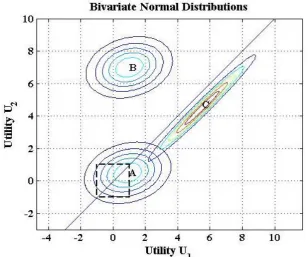
With a fixed covariance matrix, we illustrate the impact of generating the mean, , from different ranges. Figure 1 shows three bivariate utility distributions (A, B, C). Sampling each component of the mean from

([ ]), as marked by the dashed square, would result in distributions such as A. The distribution straddles the diagonal and hence both alternatives have significant (non-zero) choice probabilities. With the same covariance matrix, randomly sampling the components of the mean from a larger range such as ([ ]) often results in a distribution located like B, where the choice probabilities will be 0/1 even to the maximum accuracy we might hope to attain. Such cases do not rely on highly accurate estimation of that part of the PDF above or below the diagonal. Correlations between alternatives are also influential, and may raise or lower the chance of selecting the alternative with lower mean utility. The strong positive correlation between alternatives in distribution C increases the probability of choosing alternative 1, in comparison with having independent alternatives.

In our tests, we sample the mean for the MVN distribution from ([ ] ), where the number of alternatives is . Initial tests indicated that the accuracy of the ME and SJ approximation methods may depend on the (relative) size of the off-diagonal terms in the covariance matrix. With this in mind, we test

3

Page 7

covariance matrices } of the form where is the identity matrix and } are randomly generated correlation matrices (built using eigenvalues randomly drawn from a uniform distribution). The scalar therefore parameterises the relative magnitude of the variances compared with the (off-diagonal) correlations. Increasing increases the magnitude of the diagonal terms, without changing the off-diagonal/correlation terms.

Figure 1: Range for sampling the mean utility

Distributions plotted

([ ] [ ])

([ ] [ ])

([ ] [ ])

We test values of and labelled { } and }. Increasing leads to the occurrence of more near 0/1 probabilities as described above. Increasing amplifies the diagonal terms, which dominate the covariance matrix i.e. larger corresponds to effectively smaller correlations. The tests are built from several components

I. The number of alternatives (for each choice) determines the problem dimension . II. Given we generate a set of correlation matrices }.

III. Given , we draw mean vectors from the uniform distribution ([ ] ).

IV. Given , we compute the choice probabilities for ( ) by each method, for each of the pairs .

V. For each method, we compute the error in each individual choice probability (there are ). Hence for each problem dimension , at each setting of and we compute the choice probabilities for MVN distributions. With N alternatives, the choice probabilities for a given ( ) is an

N-vector: from “exact” computation (using MATLAB’s mvncdf function), from the SJ approximation, via ME and the three Monte Carlo methods , and .

The ‘exact’ choice probabilities were computed to an accuracy of 1E-4 in MATLAB. These values are used to calculate errors in the choice probabilities computed by other methods, for example the ME errors are

. Errors below 1E-4 cannot therefore be regarded as precise.

3.2. Role of Internal Averaging

Page 8

also establish a number of draws for each Monte Carlo method that offers reasonable comparison with the analytical approximation methods.

We generated a set of 25 choice situations: ( ), . Each drawn from

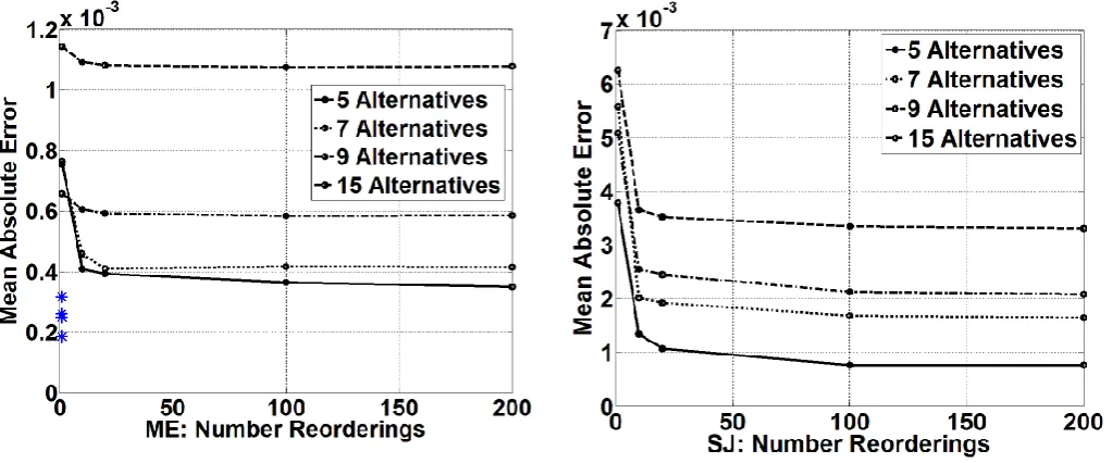
([ ] ), each drawn from ([ ]) and } generated as described above. For these 25 choice problems, the choice probabilities were computed using each method and mean absolute error across all situations calculated. This was repeated for numbers of choice alternatives . Figure 2 and Figure 3 show the dependency of errors in the choice probabilities on the number of re-orderings included in the average.

For both SJ and ME methods, various non-random orderings were also tested (prompted by Langdon 1984b); specifically, the terms in (11) were ordered by increasing or decreasing } before writing expressions (13) and (15). For the ME method, the order of decreasing } was found to be effective. ME using this single optimal order of terms is labelled ‘MEO’. For the SJ method decreasing } made a slight improvement, but averaging over multiple random orderings was much more effective than any single ordering. For both ME and SJ, [1,10,20,100,200] random re-orderings were tested.

Figure 2: ME error with internal averaging.

Asterisks indicate MEO error (for N=5,7,9,15). Figure 3: SJ error with internal averaging.

Many more tests were performed that confirm the trends shown here: internal averaging significantly improves the accuracy of SJ, much less so for ME. ME outperforms SJ (note y-scale in Figures 2 & 3) in fact the ME method with no averaging (any random single internal ordering of terms) is often more accurate than the SJ method with all permutations included (note y-axis scales in the Figures). MEO with the single optimal ordering of terms (lines without markers in Figure 2) significantly outperforms unordered ME.

Page 9

Similar tests were run to determine appropriate numbers of draws for the three Monte Carlo based methods (Figure 4). For the GZ method the tests examined [50, 200, 500, 1000, 5000] draws. For GHK [500, 5000, 10000, 25000, 50000] draws were tested and for the FB approach [1000, 5000, 25000, 50000, 100000] draws were considered.

Based on these findings, the tests that follow in the next section consider only the single optimal ordering of terms for ME, labelled MEO. For SJ we report tests using 10 internal re-orderings, labelled SJ10; averaging over 10 random re-orderings improves accuracy appreciably. No more re-orderings were included as execution time increases with each additional reordering. For the Monte Carlo methods, the simple frequency based MC is run using 50,000 draws (labelled FB50k), GHK with 10,000 draws (labelled GHK10k), and the quasi-MC method of Genz is run with 500 draws (labelled GZ500). These selections are a compromise between accuracy and computation time and were chosen to give the best comparison with MEO in the tests below.

3.3. Comparison of Computation Speed With Precision

We now test the trade off between execution speed and accuracy across a wide range of settings. Considered in turn are . For each problem dimension N, we consider 17 settings of the utility range

, and 19 values for the (relative) magnitude of variance :

}

}

At each setting ( ) we draw values for the deterministic utility ( ) and generate covariance matrices (having diagonal elements ); the choice probabilities are then computed for these MVN distributions via each method. We use , hence for each problem dimension, , we compute choice probabilities for 8075 MVN distributions. Tests extending beyond these parameter ranges did not reveal any substantial new insights.

Table 1: Summary of Execution Times and Errors. The data for each problem dimension [5,7,9,15 alternatives] come from 8075 choice situations, ranging over different specifications of mean and

covariance (see Section 3.1)

nAlt MEO GZ 500 GHK 10k FB 50k SJ10 ML

5

Time per choice (s) 0.0014 0.0303 0.0871 0.0226 0.0292 0.6580

Time per choice (x MEO) 1 22 63 16 21 477

Errors > 1E-4 69% 38% 47% 92% 86% 0%

Errors > 0.001 0.9% 0.0% 2.3% 48.8% 39.3% 0%

7

Time per choice (s) 0.0029 0.0703 0.1974 0.0316 0.0846 2.2461

Time per choice (x MEO) 1 25 69 11 30 788

Errors > 1E-4 55% 51% 47% 90% 91% 0%

Errors > 0.001 0.8% 0.1% 2.4% 42.6% 55.8% 0%

9

Time per choice (s) 0.0048 0.1265 0.3487 0.0367 0.1811 4.3376

Time per choice (x MEO) 1 26 73 8 38 906

Errors > 1E-4 50% 56% 46% 88% 92% 0%

Errors > 0.001 0.8% 0.8% 2.5% 37.9% 62.3% 0%

15

Time per choice (s) 0.014 0.42 1.24 0.064 0.878 22.224

Time per choice (x MEO) 1 30 88 5 63 1584

Errors > 1E-4 61% 62% 42% 84% 92% 0%

Errors > 0.001 0.3% 3.6% 1.8% 28.3% 68.0% 0%

Page 10

MEO with optimal ordering is always the quickest method, and is more than 20 times faster than any of the methods that give comparable accuracy. FB50k improves in its speed relative to MEO, though is still four times slower at and five times less precise.

The execution time of every method increases with problem dimension. The execution time of methods ML, SJ10, GHK10k not only increase, but also worsen significantly in comparison with MEO. The relative speed of GZ500 also gets slightly worse compared to MEO as the problem dimension increases. Not surprisingly the execution time of FB scales best with and its accuracy does not degrade appreciably, though it is one of the least accurate methods throughout (with this number of draws).

The most accurate methods are MEO, GHK10k and GZ500, though the latter is consistently 20x-30x slower. For , GZ500 offers the highest level of accuracy, with more than half of all points having errors within the range of the ‘exact’ ML method. For , the MEO and GZ500 methods are comparable in accuracy, and at & 15 we see that MEO has eclipsed the accuracy of GZ500. MEO is more than 25 times faster in both cases. GHK10k also competes well in terms of accuracy, especially at higher dimensions, but is 60-80 times slower than MEO. Perhaps GZ with more draws could compete in terms of accuracy and speed with GHK.

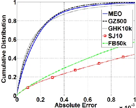
From the same data, we plot the cumulative distributions of absolute errors in the individual choice probabilities in Figures 2-5 for respectively. The lines showing the distribution of errors for MEO, GZ500 and GHK10k are close together with more than half the errors below 2E-3, while the absolute errors for SJ10 and FB50k are substantially larger. Note the errors for MEO are greater than GZ500 and GHK10k for , these methods are almost equivalent for while for GHK10k appears more accurate (though 88 times slower than MEO).

Page 11

Figure 7: Choices with 9 alternatives Figure 8: Choices with 15 alternatives

Next we examine whether or not the errors are dependent on the values of and . Recall that the mean is sampled from ([ ] ) with larger increasing the occurrence of 0/1 probabilities, while controls dominance of the diagonal terms in the covariance matrix. At each setting ( ) we compute the mean absolute error across the individual choice probabilities. For , contours of these mean absolute errors are plotted in Figure 4. The tests with 5, 9 and 15 alternatives reveal a similar pattern in the errors for each method.

Figure 9: Mean absolute error for choices with 7 alternatives at different settings for the mean and covariance of the underlying MVN pdf.

Page 12

choice situations tested, doing less well only in a region near to the origin, where so that correlations dominate the covariance matrix. In this specific region, GZ500 and GHK10k perform better; this was similarly the case for . Methods GZ500 and GHK10k in particular display a distinct overall trend in errors, which was noticeable across all problem dimensions tested. This indicates values of and where one of these methods might be preferred over the other, though computation time also should be considered. Plots (not displayed here) of the maximum error for any individual choice probability, reveal similar patterns of performance to those shown in Figure 9.

It is worth noting a potential weakness of the SJ method that arises from the need to invert a matrix relating to the covariance. Computing the probabilities via SJ (using the algorithm described in Joe 1995) can lead to ill conditioning of this matrix and hence inaccurate results. This can lead to inaccurate results from SJ. It may be possible to design a different algorithmic implementation of the SJ approach to guard against this problem, but this is outside the scope of this paper.

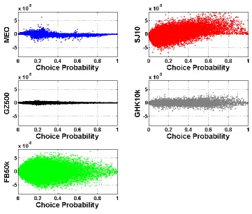
3.4. Distribution of Error with Individual Probability Value

We now investigate whether there are systematic errors with probability value, with a view to determining, for example, if small probabilities are always under or over-estimated. The errors in every individual choice probability from the tests above are plotted in turn in the figures below. There are points on each such plot.

The distribution of errors may not be clear due to the concentration of the plotted points, hence refer to Figures 2-5. All sets of axes have the same scale to aid comparison. Similar plots of the errors for 7 and 15 alternatives do not reveal any substantial new insights.

Figure 10: Error with choice probability value for choice situations with 5 alternatives

Page 13

Figure 11: Error with choice probability value for choice situations with 9 alternatives

3.5. Computing Derivatives

As Daganzo (1979, p72) explains (attributed to McFadden, 1978b), the (off diagonal) partial derivatives of the choice probabilities can be expressed exactly as the choice probability from a probit model with one fewer alternative, i.e.:

( ) (

| ( )|

| |) ( ( )) ( ( ) ( )) (18)

where if , if and ( ) ( ) ( ) are simple transformations of and with the jth rows and columns removed.The diagonal terms can then be computed immediately from the off-diagonal derivatives. Hence fast and accurate calculation of the derivatives is equivalent to fast and accurate calculation of the choice probabilities as presented above.

For the estimation of choice models, the derivatives of the log-likelihood function are of interest, therefore requiring first derivatives of the choice probabilities with respect to the preference parameters. These are easily constructed from the above result. Similarly, in traffic networks, sensitivity analysis of the equilibrium flows can be an important tool and this relies on the Jacobian of the choice probabilities exactly as written above (see for example Connors et al., 2007).

For completeness, we also briefly present results showing the accuracy of using numerical differences to approximate these partial derivatives, when the choice probabilities being differenced have been calculated using MEO, SJ or via Monte Carlo. As before, we consider 100 distributions ( ); effectively a subsample of the scenarios investigated in the tests above (sections 3.3 and 3.4). The matrices

} are randomly generated correlation matrices as before, with drawn from ([ ]). The mean utilities are drawn from ([ ] ). For each , we construct the difference matrix as follows (shown here for to conserve space):

[

( ) ( ) ( ) ( ) ( ) ( ) ( ) ( ) ( ) ( ) ( ) ( ) ( ) ( ) ( ) ( ) ( ) ( )

Page 14

where [ ] with a one in the ith place. This approximate Jacobian is calculated using choice probabilities according to each of the above methods.

As noted earlier, errors in the ‘exact’ method may influence the results hen differencing small probabilities. To account for this, we record how many choice probabilities are sufficiently small that they are within the computational error 1E-4 of the ‘exact’ method. The errors computed are mean absolute error and max absolute error averaged over all tested choice situations (100 for each of 5, 7 and 9 alternatives). The results shown in Table 2 depend on the value of used to compute the differences. All tests show that SJ is the least accurate method. FB50k and MEO are similarly accurate for , while MEO offers improved accuracy at and . Meanwhile, methods GZ500 and GHK10k are very much more accurate in computing these derivatives than all other methods tested, although it should be noted that any speed penalty is increased by times in computing these numerical differences. For 5,7 and 9 alternatives this implies GZ500 will be 110,175 and 234 times slower than MEO while GHK10k will be 315,483 and 657 times slower.

Table 2: Approximating derivatives by numerical differencing: mean absolute error over 100 computations with interval .

nAlt 5 7 9

40% 50% 62%

MEO

[ ] [0.0319 0.0032 0.0003] [0.0240 0.0024 2.9E-4] [0.0263 0.0026 3.0E-4]

SJ10

[ ] [1.1519 0.1168 0.0119] [1.5407 0.1556 0.0154] [1.8384 0.1823 0.0182]

FB50k

[ ] [0.0369 0.0066 0.0019] [0.0283 0.0050 0.0013] [0.0287 0.0043 0.0011]

GZ500

[ ] [3.1E-4 3.1E-5 3.1E-6] [2.7E-4 2.7E-5 2.5E-6] [2.7E-4 2.7E-5 2.7E-6]

GHK10k

[ ] [3.1E-4 3.1E-5 3.2E-6] [2.7E-4 2.7E-5 2.7E-6] [2.7E-4 2.7E-5 3.1E-6]

4. Conclusion

In this paper we have compared two analytical approximations and three Monte Carlo methods for computing the probit choice probabilities in terms of accuracy and computational efficiency. The first of these is the “Solo -Joe” (SJ) approach, implemented using the algorithm proposed in Joe (1995). The other is the “Mendell-Elston” (ME) approach, as described in Kamakura (1989). While it is not possible to be exhaustive, the results presented here give what we believe to be the most thorough and in-depth comparison of these analytical approximation methods to date in the context of multinomial probit choice. The results should be of interest to both network modellers and choice modellers, not least given the renewed interest in probit among the latter, where recent CML developments have adopted the SJ approach.

Page 15

Especially in model estimation, chosen alternatives with very small probabilities can have a disproportionate impact, making accurate calculation of such probabilities essential. The results from Section 3.4 show the spread of errors across the computed choice probabilities. We note that ME is more accurate in computing small probabilities than SJ or MC, and is comparable with GZ and GHK doing worse for and as well or better for .

It is important to acknowledge that there are many parameter dimensions to test in assessing whether one approximation method is more accurate than another. The tests reported here are an illustrative selection of all tests performed in this research. Each analytic approximation method suffers from the disadvantage that the analyst cannot demand arbitrary accuracy, whereas in principle this is possible via MC, GZ and GHK. Moreover, we cannot offer bounds for the errors of these methods. Finally, for problems with a very small number of alternatives, exact evaluation of choice probabilities is computationally feasible using established methods of numerical integration. For higher dimensional problems, ME is an accurate and efficient method for computing choice probabilities.

With the strength of the results presented here, it seems that the wider use of the “Mendell-Elston” method in probit work, and implementation within a composite marginal likelihood estimator are thus promising areas for new developments. While the primary motivation for this paper is to help with the estimation and application of discrete choice models, there may also be applications in other areas where the computation of multivariate normal integrals is needed.

Acknowledgment

This work described in this paper was supported by the UK Engineering and Physical Sciences Research Council (EPSRC) through the project “Estimation of travel demand models from panel data” grant EP/G033609/1. The second author also acknowledges the support of the Leverhulme Trust in the form of a Leverhulme Early Career Fellowship.

Bibliography

Aitken, A.C., 1935. Note on selection from a multivariate normal population. Proceedings of the Edinburgh Mathematical Society 4, 106–110.

Bolduc, D., 1999. A practical technique to estimate multinomial probit models in transportation. Transportation Research Part B: Methodological 33, 63–79.

Bhat, C., 2001, Quasi-random maximum simulated likelihood estimation of the mixed multinomial logit model, Transportation Research B 35, 677–693.

Bhat, C.R., 2010. The maximum approximated composite marginal likelihood (MACML) estimation of mixed unordered response choice models. Technical Paper, Department of Civil, Architectural, and Environmental Engineering, The University of Texas at Austin, Austin, Texas.

Bhat, C.R., Sidharthan, R., 2010. A Simulation Evaluation of the Maximum Approximated Composite Marginal Likelihood (MACML) Estimator for Mixed Cross-Sectional and Panel Unordered Response Choice Models.

Bhat, C.R., Varin, C., Ferdous, N., 2010. A comparison of the maximum simulated likelihood and composite marginal likelihood estimation approaches in the context of the multivariate ordered response model system. Advances in Econometrics: Maximum Simulated Likelihood Methods and Applications 26. Börsch-Supan, A., Hajivassiliou, V., 1993. Smooth unbiased multivariate probability simulators for

maximum likelihood estimation of limited dependent variable models* 1. Journal of econometrics 58, 347–368.

Bunch, D.S., 1991. Estimability in the multinomial probit model. Transportation Research Part B: Methodological 25, 1–12.

Page 16

stochastic user equilibrium with multiple user-classes. Transportation Research Part B: Methodological 41, 593–615.

Daganzo, C., 1979. Multinomial probit: The theory and its application to demand forecasting. Academic Press New York: NY.

Dalal, S.R. and Klein, R.W., 1988, A Flexible Class of Discrete Choice Models. Marketing Science, Vol. 7, 232-251.

Dansie, B.R., 1985. Parameter estimability in the multinomial probit model. Transportation Research Part B: Methodological 19, 526–528.

Drezner, Z. 1990. Approximations to the Multivariate Normal Integral. Communications in Statistics – Simulation and Computation, 19, 527-534.

Drezner, Z., 1994. Computation of the trivariate normal integral. mathematics of computation 62, 289–294. Drezner, Z., Wesolowsky, G.O., 1990. On the computation of the bivariate normal integral. Journal of

Statistical Computation and Simulation 35, 101–107.

Genz, A., 1992. Numerical computation of multivariate normal probabilities. Journal of computational and graphical statistics 1, 141–149.

Genz, A., Bretz, F., 1999. Numerical computation of multivariate t-probabilities with application to power calculation of multiple contrasts. Journal of Statistical Computation and Simulation 63, 103–117. Genz, A., Bretz, F., 2002. Comparison of methods for the computation of multivariate t probabilities.

Journal of Computational and Graphical Statistics 11, 950–971.

Genz, A., 2004. Numerical computation of rectangular bivariate and trivariate normal and t probabilities. Statistics and Computing 14, 251-260.

Hess, S., Train, K.E. & Polak, J.W. (2006), On the use of a Modified Latin Hypercube Sampling (MLHS) approach in the estimation of a Mixed Logit model for vehicle choice, Transportation Research Part B, 40(2), pp. 147-163.

Joe, H., 1995. Approximations to Multivariate Normal Rectangle Probabilities Based on Conditional Expectations. Journal of the American Statistical Association 90, 957-964.

Kamakura, W.A., 1989. The Estimation of Multinomial Probit Models: A New Calibration Algorithm. Transportation Science 23, 253-265.

Keane, M.P., 1992. A note on identification in the multinomial probit model. Journal of Business & Economic Statistics 10, 193–200.

Langdon, M.G., 1984a. Improved algorithms for estimating choice probabilities in the multinomial probit model. Transportation Science 18, 267.

Langdon, M.G., 1984b. Methods of determining choice probability in utility maximising multiple alternative models. Transportation Research Part B: Methodological 18, 209–234.

Lee, L., 1992, On the efficiency of methods of simulated moments and simulated likelihood estimation of discrete choice models, Econometric Theory 8, 518–552.

Lee, L., 1995, Asymptotic bias in simulated maximum likelihood estimation of discrete choice models, Econometric Theory 11, 437–483.

Manski, C., Lerman, S., (1981). On the use of simulated frequencies to approximate choice probabilities. Structural Analysis of Discrete Data with Econometric Applications 305–319.

McFadden, D., 1978a, Modeling the choice of residential location, in A.Karlqvist, L.Lundqvist, F.Snickars and J.Weibull eds ‘Spatial Interaction Theory and Planning Models’ North-Holland, Amsterdam, pp. 75–96.

McFadden, D., 1978b. Quantitative methods for analysing travel behaviour of individuals: Some recent developments., in: Behavioral Travel Modeling, edited by DA Hensher and PR Stopher. Croom Helm, London, pp. 279-318.

McFadden, D., 1989. A method of simulated moments for estimation of discrete response models without numerical integration. Econometrica: Journal of the Econometric Society 57, 995–1026.

McFadden, D. and Train, K.E., 2000. Mixed mnl models of discrete response, Journal of Applied Econometrics 15, 447–470.

Mendell, N., Elston, R., 1974. Multifactorial Qualitative Traits - Genetic-Analysis And Prediction Of Recurrence Risks. Biometrics 30, 41-57.

Page 17

Rosa, A., 2003. Probit Based Methods in Traffic Assignment and Discrete Choice Modelling, unpublished. Solow, A.R., 1990. A method for approximating multivariate normal orthant probabilities. Journal of

Statistical Computation and Simulation 37, 225–229.

Sumalee, A., Uchida, K., Lam, WHK. 2009 .Stochastic Multi-Modal Transport Network Under Demand Uncertainties and Adverse Weather Condition, 18th International Symposium On Transportation And Traffic Theory, 19-41.

Teng, H., Qi, Y., Martinelli, D.R. 2008. Parking difficulty and parking information system technologies and costs. Journal Of Advanced Transportation 42(2), 151-178.

Thurstone, L., 1927. A law of comparative judgment. Psychological Review 34, 273-286.

Train, K. 2000, Halton sequences for mixed logit, Working Paper No. E00-278, Department of Economics, University of California, Berkeley.

Train, K.E. 2009. Discrete choice methods with simulation, Second Edition. Cambridge University Press, Cambridge, MA.