Rochester Institute of Technology
RIT Scholar Works
Theses Thesis/Dissertation Collections
9-21-2015
Heavy Ball with Friction Method for the
Elastography Inverse Problem
Oladayo Eluyefa
Follow this and additional works at:http://scholarworks.rit.edu/theses
This Thesis is brought to you for free and open access by the Thesis/Dissertation Collections at RIT Scholar Works. It has been accepted for inclusion in Theses by an authorized administrator of RIT Scholar Works. For more information, please [email protected].
Recommended Citation
Heavy Ball with Friction Method for
the Elastography Inverse Problem
By
Oladayo Eluyefa
A thesis submitted in partial fulfillment of the requirements for the degree of Master of Science
in Applied and Computational Mathematics from the School of Mathematical Sciences
College of Science
Rochester Institute of Technology
September 21, 2015
Advisor: Dr. Akhtar Khan
Co-Advisor: Dr. Baasansuren Jadamba Committee members: Dr. Patricia Clark
Committee Approval:
Akhtar A. Khan
School of Mathematical Sciences Thesis Advisor
Date
Baasansuren Jadamba
School of Mathematical Sciences Thesis Co-advisor
Date
Patricia Clark
School of Mathematical Sciences Committee Member
Date
Bonnie Jacob
Science and Mathematics Department, NTID Committee Member
Date
Elizabeth Cherry
School of Mathematical Sciences Director of Graduate Programs
Abstract
The primary objective of this thesis is to develop a fast and efficient compu-tational framework for the nonlinear inverse problem of identifying a variable coefficient in a system of partial differential equation modelling the response of an incompressible elastic object under some known body forces and bound-ary traction. The main novelty of this contribution is to use, for the first time, of the so-called heavy ball with friction method for inverse problems. The heavy ball with friction dynamical system is a nonlinear oscillator with damping. The key idea is to pose the inverse problem as an optimization problem, derive its optimality system, and then seek the solution through a trajectory of a dynamical system. In this work, we will study four differ-ent optimization formulations for the nonlinear inverse problem and thor-oughly compare their convergence and numerical performance. Since we use a second-order method, we also investigate a general second-order hybrid and a second-order adjoint method for an efficient computation of the hessian of the output least-squares formulation. The stability of the dynamical system approach with respect to the contamination in the data is thoroughly inves-tigate in the context of a simpler elliptic partial differential equation. The mixed finite element approach is used to discretize the direct as well as the inverse problems.
Dedication
I would like to dedicate this to my family for supporting me unfailingly throughout my studies.
Acknowledgement
I would like to thank my family, friends, and mentors for helping me through this learning process, your support was vital to my success.
I am especially grateful to my advisors, Dr. Akhtar Khan and Dr. Baasansuren Jadamba. They have been extremely supportive of me throughout my time in school even before our research began. Their guidance and support has helped me grow and learn valuable skills not only in mathematics, but also in life.
I would also like to thank the School of Mathematical Sciences within the College of Science at RIT for their help throughout my time here. I would like to thank, in particular, Anna Fiorucci, and Carrie Koneski who have been instrumental throughout this journey.
Most importantly, I would like to thank my parents for their encouragement and support. Without them, none of this would be possible. I love my family very much.
Contents
1 Introduction 2
1.1 Motivation . . . 2
1.2 The Inverse Problem . . . 3
1.3 Literature Review . . . 3
1.4 Objectives and Structure . . . 5
2 Various Optimization Schemes 6 2.1 Saddle Point Formulation . . . 6
2.2 Output Least Squares . . . 8
2.2.1 First Order Derivative . . . 9
2.2.2 Second Order Derivative . . . 11
2.3 Modified Output Least Squares . . . 15
2.4 Energy Output Least Squares . . . 16
2.5 Equation Error Approach . . . 17
3 Discretization 19 3.1 Finite Element Discretization . . . 19
3.2 Discrete Optimizers . . . 21
3.2.1 Discrete Output Least Squares . . . 21
3.2.2 Discrete MOLS . . . 25
3.2.3 Discrete EOLS . . . 25
3.2.4 Discrete Equation Error . . . 26
4 Heavy Ball with Friction Method 27 4.1 Introduction . . . 27
4.2 Continuous Methods . . . 27
4.2.1 A Continuous Newton-Type Trajectory . . . 28
4.3 Heavy Ball with Friction Method . . . 29
5 Numerical Experiments 32 5.1 Introduction . . . 32
5.2 Computations using OLS . . . 34
5 CONTENTS
5.3.1 Computations using MOLS . . . 36
5.3.2 Computations using EOLS . . . 38
5.3.3 Computations using Equation Error . . . 41
5.4 Choice of Parameters for HBF . . . 43
6 Performance of Differential Equations Based Solvers for Noisy Data 45 6.1 Motivation . . . 45
6.2 Objective and Approach . . . 45
6.3 Model Problem . . . 46
6.4 Optimization Formulations . . . 46
6.4.1 Output Least Squares . . . 46
6.4.2 Modified Output Least Squares . . . 47
6.4.3 Equation Error . . . 48
6.5 Numerical Experiments . . . 49
6.5.1 Computations using OLS . . . 50
6.5.2 Computations using MOLS . . . 52
6.5.3 Computations using Equation Error . . . 63
6.6 A Comparative Analysis of the Noisy Data . . . 73
List of Figures
5.1 Example 1 OLS Hybrid . . . 34
5.2 Example 1 OLS Adjoint . . . 34
5.3 Example 2 OLS Hybrid . . . 35
5.4 Example 2 OLS Adjoint . . . 35
5.5 Example 1 MOLS CG . . . 36
5.6 Example 2 MOLS CG . . . 37
5.7 Example 1 MOLS HB . . . 37
5.8 Example 2 MOLS HB . . . 38
5.9 Example 1 EOLS CG . . . 39
5.10 Example 2 EOLS CG . . . 39
5.11 Example 1 EOLS HB . . . 40
5.12 Example 2 EOLS HB . . . 40
5.13 Example 1 EE CG . . . 41
5.14 Example 2 EE CG . . . 42
5.15 Example 1 EE HB . . . 42
5.16 Example 2 EE HB . . . 43
6.1 Example 2 PTC OLS Hybrid . . . 51
6.2 Example 2 PTC OLS Adjoint . . . 51
6.3 Example 3 PTC OLS Hybrid . . . 51
6.4 Example 3 PTC OLS Adjoint . . . 52
6.5 Example 1 Euler CG . . . 53
6.6 Example 1 Trap CG . . . 53
6.7 Example 1 RK CG . . . 53
6.8 Example 1 ode113 CG . . . 54
6.9 Example 1 Euler HB . . . 54
6.10 Example 1 Trap HB . . . 55
6.11 Example 1 RK HB . . . 55
6.12 Example 1 ode113 HB . . . 55
6.13 Example 2 Euler CG . . . 56
6.14 Example 2 Trap CG . . . 56
7 LIST OF FIGURES
6.16 Example 2 ode113 CG . . . 57
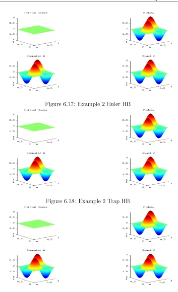
6.17 Example 2 Euler HB . . . 58
6.18 Example 2 Trap HB . . . 58
6.19 Example 2 RK HB . . . 58
6.20 Example 2 ode113 HB . . . 59
6.21 Example 3 Euler CG . . . 59
6.22 Example 3 Trap CG . . . 60
6.23 Example 3 RK CG . . . 60
6.24 Example 2 ode113 CG . . . 60
6.25 Example 3 Euler HB . . . 61
6.26 Example 3 Trap HB . . . 61
6.27 Example 3 RK HB . . . 62
6.28 Example 3 ode113 HB . . . 62
6.29 Example 1 Euler CG . . . 63
6.30 Example 1 Trap CG . . . 63
6.31 Example 1 RK CG . . . 64
6.32 Example 1 ode113 CG . . . 64
6.33 Example 1 Euler HB . . . 65
6.34 Example 1 Trap HB . . . 65
6.35 Example 1 RK HB . . . 65
6.36 Example 1 ode113 HB . . . 66
6.37 Example 2 Euler CG . . . 66
6.38 Example 2 Trap CG . . . 67
6.39 Example 2 RK CG . . . 67
6.40 Example 2 ode113 CG . . . 67
6.41 Example 2 Euler HB . . . 68
6.42 Example 2 Trap HB . . . 68
6.43 Example 2 RK HB . . . 69
6.44 Example 2 ode113 HB . . . 69
6.45 Example 2 Euler CG . . . 70
6.46 Example 3 Trap CG . . . 70
6.47 Example 3 RK CG . . . 70
6.48 Example 3 ode113 CG . . . 71
6.49 Example 3 Euler HB . . . 71
6.50 Example 3 Trap HB . . . 72
6.51 Example 3 RK HB . . . 72
6.52 Example 3 ode113 HB . . . 72
6.53 Example 2 MOLS vs EE Noise = 10−3 . . . 73
6.54 Example 2 MOLS vs EE Noise = 10−2 . . . 74
6.55 Example 2 MOLS vs EE Noise = 5·10−2 . . . 74
6.56 Example 2 OLS vs. MOLS vs. EE Noise = 5·10−2 . . . 76
8 LIST OF FIGURES
6.58 Example 2 OLS vs. MOLS vs. EE Noise = 10−3 . . . 78
6.59 Example 3 OLS vs. MOLS vs. EE Noise = 10−1 . . . 79
6.60 Example 3 OLS vs. MOLS vs. EE Noise = 10−2 . . . 80
List of Tables
5.1 OLS Numerical Results . . . 35
5.2 MOLS Numerical Results . . . 38
5.3 EOLS Numerical Results . . . 40
5.4 EE Numerical Results . . . 43
5.5 Effect of Parameter Choice in Heavy Ball method . . . 43
6.1 Example 2 OLS PTC . . . 52
6.2 MOLS Example 1 First Order ODE . . . 54
6.3 MOLS Example 1 Second Order ODE . . . 56
6.4 MOLS Example 2 First Order ODE . . . 57
6.5 MOLS Example 2 Second Order ODE . . . 59
6.6 MOLS Example 3 First Order ODE . . . 61
6.7 MOLS Example 3 Second Order ODE . . . 62
6.8 EE Example 1 First Order ODE . . . 64
6.9 EE Example 1 Second Order ODE . . . 66
6.10 EE Example 2 First Order ODE . . . 68
6.11 EE Example 2 Second Order ODE . . . 69
6.12 EE Example 3 First Order ODE . . . 71
6.13 EE Example 3 Second Order ODE . . . 73
6.14 Example 2 - Euler Noise Study . . . 74
6.15 Example 2 - Trapezoid Noise Study . . . 75
6.16 Example 2 - Runge Kutta Noise Study . . . 75
6.17 Example 2 - ODE113 Noise Study . . . 75
6.18 Example 2 - Scheme Comparison . . . 82
Chapter 1
Introduction
This chapter introduces the concept of an inverse problem of parameter iden-tification. It also provides motivation for the research in the field of inverse problems. A literature review is performed on the ideas and concepts leading up to this work. Finally, it states the structure and objectives of the thesis work.
1.1
Motivation
Cancer is becoming one of fastest growing causes of death in the world [39]. Soft tissue cancer is but one form and it is as deadly as any other. The large number of deaths due to soft tissue cancer can be managed through early detection of the tumorous cells within a tissue that could be potentially cancerous. However, the means of identification of these tumorous cells are somewhat lacking. Palpation and ultrasound are some of the procedures currently used in the identification of such cells. Ultrasound relies on the acoustic behavior of tissue based on its physical properties, which is in turn determined by its health. Ultrasound detect differences in tissue stiffness by passing sound waves through the tissue and using the response times as an indication of this property [29]. Palpation is a procedure in which force is manually applied to a region of concern, and differences in the structure of healthy versus unhealthy cells are used to determine if an area has harder ”lumps” than its surrounding tissue [19]. A drawback of palpation is that it can only be used near the surface of the skin. Also, deciding which cell regions are classified as harder than others is very subjective.
3 1.2. The Inverse Problem
1.2
The Inverse Problem
An inverse problem arises from an underlying direct problem. Consider a mathematical system that models the heat transfer from a heat source to a metallic body. In this system, we have a heat source, the temperature of the metallic body as a function of position, and the thermal conductivity of the body. In the direct problem, the thermal conductivity and the heat source are the known terms, and the output of the direct problem is the temperature of the body. One possible inverse problem would be to calculate the amount of heat produced from the heat source, provided we know the thermal con-ductivity of the body, and we have a means of measuring the temperature of the body. This is known as the inverse problem of source identification. The other kind of inverse problem would involve identifying the thermal conductivity of the body given the heat source, and a measurement of the temperature of the body. In most mathematical systems, innate properties such as the thermal conductivity of a body are represented by parameters within the model. As a result, the latter problem is referred to as the inverse problem of parameter identification. Broadly, the inverse problem is a way of non intrusively calculating some innate characteristic of a material within a system that could otherwise not be measured. In the cancer problem, using elastic imaging, the elasticity is the innate characteristic of the tissue that is to be calculated. Some amount of force is applied, which is the source, and the output, is the displacement, which can be measured or observed. Other examples of inverse problems are studied in [12, 22, 23, 25, 32, 36, 46].
1.3
Literature Review
There has been a lot of work leading up to the ideas explored in this thesis both in the field of elasticity imaging with respect to inverse problems, and the use of dynamical systems in optimization problems. This review is in no way exhaustive, but it highlights a few works that have led up to the concepts used directly and extensively in this thesis.
Ultrasound based methods have been extensively used over time when it comes to tumor identification and elasticity imaging. Bertrand[14] and Parker et al.[40], both used ultrasound methods to try to attain the elasticity mod-ulus of a tissue. Bamber at al. [11] used ultrasound techniques to image the compressed breast in order to attain axial displacements. These meth-ods were somewhat idealized as they assumed that both the location, and geometry of the tumor were known at the start of the process.
4 1.3. Literature Review
element methods were used by Kallel and Bertrand[31] when they tried to fit the axial displacement of the compressed tissue gotten from ultrasound imaging, in a least squares sense. Doyley et al.[21] used iterative schemes to retrieve the Young’s modulus or elasticity modulus. Such work can be see in [27, 33] as well.
In 2003, Oberai et al.[38] studied the identification of the shear modulus in an incompressible elastic material.
More recently, Arnold et al.[7] developed numerical methods for identification of the elasticity modulus. In the same year, Ammari et al.[5] used optimiza-tion approaches to tackle the same problem. Doyley has a very extensive survey article on these topics[19]. More can be found in [20, 18, 13, 37, 47] In the field of continuous methods and its applications to optimization, Bostaris[15] introduced broader curvilinear search paths that used the eigen property of the Hessian matrix in function minimization. Bartholomew-Biggs and Brown[17, 16] studied trajectories based on a system of differential equa-tions to solve an equality constraint optimization problem. Sch¨affler[42] con-sidered a gradient trajectory method for optimization and fifteen years later Liao[35] considered a gradient based continuous method.
Antipin[6] did work with convex programming problems using continuous gradient projections of both the first and second order. Glazos et al.[24] presented a family of dynamical systems whose steady state solution solves a convex optimization problem. Alvarez and P´erez[4] did work on convex minimization problems using newton type continuous methods. Alvarez[2] then went on to study the dissipative dynamical system and gave results in a Hilbert space setting. He studied the asymptotic behavior of the solution to a particular dynamical system when its convex potential is bounded, and gave conditions for the convergence of the solution to a minimizer of the potential.
Attouch et al.[10] worked on dynamical systems that incorporate the gradi-ent of the functional being minimized into the dissipative dynamical system to yield a solution. They discussed the convergence analysis of the so-called heavy ball with friction problem. They presented conditions for convergence placing constraints on certain terms in the system. Shi[43] developed a multi-step method for solving the unconstrained minimization problem which en-sured stability of convergence, and linear rate of convergence under specified conditions.
Liao et al.[34] used a gradient based continuous method to solve the mini-mization problem. In [35], Liao used a continuous method for convex pro-gramming problems in which he converted the problems into variational in-equalities.
5 1.4. Objectives and Structure
case. Attouch and Alvarez[8] use the second order dissipative dynamical sys-tem - the heavy ball with friction method - to solve the same unconstrained optimization problem. Jules and Mainge[30] compared the standard proxi-mal point algorithm to the implicit discretization of the dissipative dynamical system by considering a co-coercive operator. The idea that certain parame-ters in the heavy ball with friction system have large effect on the convergence speed to a minimizer was extensively studied separately in [30] and [10].
1.4
Objectives and Structure
The main goals of this thesis work is to solve the inverse problem of parameter identification using differential equation approaches studied in [45, 48]. It also looks to consider possible extension discussed in [2, 4, 3, 9] with the heavy ball with friction method [2]. Different objective functionals are considered for the optimization scheme and the results are reported.
Chapter 2
Various Optimization Schemes
In this chapter, we introduce the system of partial differential equations that model the elasticity system. We use mixed finite element methods to derive the weak form of the system, and then formulate the optimization functionals that define the schemes to be used. We also present and derive the novel computation of the second order derivative of the Output Least Squares functional.
2.1
Saddle Point Formulation
Given the domain Ω as a subset ofR2or
R3 and∂Ω = Γ1∪Γ2as its boundary,
the following system models the response of an isotropic elastic body to the known body forces and boundary traction:
− ∇ ·σ = f in Ω, (2.1a)
σ = 2µ(u) +λdivu I, (2.1b)
u = g on Γ1, (2.1c)
σn = h on Γ2. (2.1d)
In (2.1), the vector-valued function u = u(x) is the displacement of the elastic body, f is the applied body force,n is the unit outward normal, and
(u) = 12(∇u+∇uT) is the linearized strain tensor. The resulting stress
tensor σ in the stress-strain law (2.1b) is obtained under the condition that the elastic body is isotropic and the displacement is sufficiently small so that a linear relationship remains valid. Here µ and λ are the Lam´e parameters which quantify the elastic properties of the object.
7 2.1. Saddle Point Formulation
of the displacement vector u under the assumption that the parameter λ is very large. The key idea behind the elatography inverse problem is that the stiffness of soft tissue can vary significantly based on its molecular makeup and varying macroscopic/microscopic structure (see [19]) and such changes in stiffness are related to changes in tissue health. In other words, the elas-tography inverse problem mathematically mimics the practice of palpation by making use of the differing elastic properties of healthy and unhealthy tissue to identify tumors. In most of the existing literature on elastography inverse problem, the human body is modelled as an incompressible elastic ob-ject. Although this assumption simplifies the identification process as there is only one parameter µto identify, it significantly complicates the computa-tional process as the classical finite element methods become quite ineffective due to the so-called locking effect. One of the few remedies of this situation is by resorting to mixed finite element formulation. We explain this in the following. For the time being, in (2.1), we set g = 0.For this case, the space of test functions, denoted by V, is given by:
V ={v¯∈H1(Ω)×H1(Ω) : ¯v = 0 on Γ1}.
By using the Green’s identity and the boundary conditions (2.1c) and (2.1d), we obtain the following weak form of the elasticity system (2.1): Find ¯u∈V
such that
Z
Ω
2µ(¯u)·(¯v)+
Z
Ω
λ(div ¯u)(div ¯v) =
Z
Ω
fv¯+
Z
Γ2
¯
vh, for every ¯v ∈V. (2.2)
The mixed finite elements approach then consists of introducing a pressure term p∈Q=L2(Ω)
p=λ(div ¯u), (2.3)
or equivalently,
Z
Ω
(div ¯u)q−
Z
Ω
1
λpq= 0, for every q ∈Q. (2.4)
By using relation (2.3), the weak form (2.2) reads: Find ¯u∈V such that
Z
Ω
2µ(¯u)·(¯v) +
Z
Ω
p(div ¯v) =
Z
Ω
fv¯+
Z
Γ2
¯
vh, for every ¯v ∈V. (2.5)
8 2.2. Output Least Squares
In the following we set B = L∞. Let A ⊂B be the set of all feasible
coeffi-cients which we assume to be nonempty, closed, and convex. Equations (2.4) and (2.5) can be written as follows:
a(`, u, v) +b(v, p) =m(v) ∀v ∈V (2.6a)
b(u, q)−c(p, q) = 0 ∀q∈Q (2.6b)
where
a(µ, u, v) =
Z
Ω
2µ(u)·(v),
b(v, p) =
Z
Ω
p(divv),
b(u, q) =
Z
Ω
(divu)q,
c(p, q) =
Z
Ω
1
λpq,
m(v) =
Z
Ω
f v+
Z
Γ2
vh.
(2.7)
It is easy to verify that a:B ×V ×V →R is trilinear and symmetric with respect to its last two arguments, b:V ×Q→R is bilinear, c:Q×Q→R
is symmetric and bilinear, and m:V →R is a linear continuous map. We assume that constants, k0, k1, k2, c1, c2 >0, exist such that
a(`, v, v)≥k1||v||2, |a(`, u, v)| ≤k2||l||||u||||v||,
c(q, q)≥c1||q||2, |c(p, q)| ≤c2||p||||q||, |b(v, q)| ≤k0||v||||q||,
(2.8)
for every ` ∈ A, u, v ∈ V, p, q ∈ Q. It is important to note that, in the following sections, since the pressure term p is also unknown, we would be stating the weak form in such a way that we look to find ¯u= (u, p) for the saddle point problem.
2.2
Output Least Squares
9 2.2. Output Least Squares
JOLS(`) =
1
2||u(`)−z¯||
2 V +
1
2||p(`)−zˆ||
2 Q
where ˆV =V ×Q, for the saddle point problem (SPP).
Inverse problems are highly ill-posed posed, meaning that the existence, uniqueness, and stability of a solution cannot be guaranteed. As a result, regularization is employed in order to attain a stable version. This ultimately yields the following optimization problem:
min
`∈A JOLS(`) =
1
2||u¯(`)−z||
2 ˆ
V +κR(`) (2.9)
where R is the regularization functional, and κ > 0 is the regularization parameter.
Now that we have derived our OLS functional, we look to compute the first order and second order derivatives of the functional. We compute the first order derivative using the first order adjoint method, and we compute the second order derivative using the second order adjoint method, and the hy-brid method.
2.2.1
First Order Derivative
Here, we use the first order adjoint method for the computation of the first derivative of the regularized OLS functional. Recall, the OLS funtional
JOLS(`) =
1
2||u(`)−z¯||
2 V +
1
2||p(`)−zˆ||
2
Q+κR(`).
This functional can be written in terms of the inner products of the spaces in which they exist to get
JOLS(`) =
1
2hu(`)−z, u¯ (`)−z¯i+ 1
2hp(`)−z, pˆ (`)−zˆi+κR(`)
By using the chain rule, the derivative ofJOLS at`∈Ain the directionδ`∈A
is given by
DJOLS(`)(δ`) =hDu(`)(δ`), u(`)−z¯i+hDp(`)(δ`), p(`)−zˆi+κDR(`)(δ`),
whereDu¯(`)(δ`) = (Du(`)(δ`), Dp(`)(δ`)) is the derivative of the coefficient-to-solution map ¯u and DR(`)(δ`) is the derivative of the regularizer R, both computed at ` in the direction δ`.
For an arbitrary ¯v = (v, q)∈V ,ˆ we define the functional ˜JOLS : B×Vˆ →R
by
˜
10 2.2. Output Least Squares
Since ¯u(`) = (u(`), p(`)) is the solution of saddle point problem (2.6), we have that
˜
JOLS(`,¯v) =JOLS(`), ∀v¯∈V .ˆ
Consequently, for every ¯v ∈Vˆ, the following identity holds
∂J˜OLS
∂` (`,¯v) (δ`) = DJOLS(`) (δ`), for every δ`∈A. (2.10)
The adjoint method is used to avoid the direct computation ofδu¯=Du¯(`)(δ`), by choosing ¯v ∈Vˆ appropriately.
∂J˜OLS
∂` (`,¯v) (δ`) = hDu(`)(δ`), u−z¯i+hDp(`)(δ`), p−zˆi
+κDR(`)(δ`) +a(δ`, u, v) +a(`, Du(`)(δ`), v) +b(v, Dp(`)(δ`)) +b(Du(`)(δ`), q)−c(Dp(`)(δ`), q).
(2.11)
For`∈A, letw(`) = ( ¯w(`), pw(`)) be the unique solution of the saddle point
problem
a(`,w, v¯ ) +b(v, pw) = hz¯−u, vi, for every v ∈V, (2.12a)
b( ¯w, q)−c(pw, q) = hzˆ−p, qi, for every q∈Q, (2.12b)
where the right-hand sides of (2.12a) and (2.12b) include the solution (u, p) of (2.6) for the given parameter, `, and data, (¯z,zˆ).
By plugging ¯v = ( ¯w, pw) in (2.11), we obtain
∂J˜OLS
∂` (`, w) (δ`) =hDu(`)(δ`), u−z¯i+hDp(`)(δ`), p−zˆi
+κDR(`)(δ`) +a(δ`, u,w¯) +a(`, Du(`)(δ`),w¯)
+b( ¯w, Dp(`)(δ`)) +b(Du(`)(δ`), pw)−c(Dp(`)(δ`), pw)
=κDR(`)(δ`) +a(δ`, u,w¯),
where we used the symmetry of a and c and the fact that w satisfies (2.12). Therefore, using (2.10), we obtain the following formula for the first-order derivative of JOLS:
DJOLS(`) (δ`) =κDR(`)(δ`) +a(δ`, u,w¯). (2.13)
Therefore, in order to compute the derivativeDJOLS(`) (δ`) of the OLS
func-tional, given`, δ`∈A, we first compute ¯u(`) = (u(`), p(`)) using (2.6). Next, we find w(`) = ( ¯w(`), pw(`)) by solving the system in (2.12), and finally we
11 2.2. Output Least Squares
2.2.2
Second Order Derivative
We compute the second order derivative of the OLS functional using two different methods: the Hybrid method and the second-order Adjoint method.
2.2.2.1 Hybrid Method for Second Derivative Computation
We aim to compute the second order derivative of the regularized OLS func-tional in such a way that we can avoid the computation of the second order derivative of the solution map ¯u. This method is referred to as the hybrid method because the derivative, δu¯ is computed using a direct method, and the computation of the second derivativeδ2u¯is avoided using an adjoint type method.
The hybrid method is based on the following result;
For each ` in the interior of A, ¯u = ¯u(`) = (u(`), p(`)) is infinitely differ-entiable at `. The first derivative δu¯ = (δu, δp) = (Du(`)δ`, Dp(`)δ`) is the unique solution of the saddle point problem:
a(`, δu, v) +b(v, δp) = −a(δ`, u, v), for every v ∈V, (2.14a)
b(δu, q)−c(δp, q) = 0, for every q∈Q. (2.14b)
Let δ`2 ∈A be a fixed direction. For any ¯v = (v, q)∈Vˆ, we define
H(`,¯v) =DJOLS(`)(δ`2) +a(`, Du(`)(δ`2), v) +b(v, Dp(`)(δ`2))
+b(Du(`)(δ`2), q)−c(Dp(`)(δ`2), q) +a(δ`2, u, v)
=hDu(`)(δ`2), u−z¯i+hDp(`)(δ`2), p−zˆi+κDR(`)(δ`2)
+a(`, Du(`)(δ`2), v) +b(v, Dp(`)(δ`2)) +b(Du(`)(δ`2), q) −c(Dp(`)(δ`2), q) +a(δ`2, u, v).
Thus, for every ¯v ∈V ,ˆ we have
∂H
∂` (`,v¯)(δ`1) =D
2
JOLS(`)(δ`1, δ`2), for every δ`1 ∈A. (2.15)
Computing this derivative of H in the direction δ`1 directly, we have
∂H
∂` (`,v¯)(δ`1) =
D2u(`)(δ`1, δ`2), u−z¯
+hDu(`)(δ`2), Du(`)(δ`1)i
+D2p(`)(δ`1, δ`2), p−zˆ
+hDp(`)(δ`2), Dp(`)(δ`1)i
+κD2R(`)(δ`1, δ`2) +a(δ`1, Du(`)(δ`2), v)
+a(`, D2u(`)(δ`1, δ`2), v) +b(v, D2p(`)(δ`1, δ`2))
+b(D2u(`)(δ`1, δ`2), q)−c(D2p(`)(δ`1, δ`2), q)
12 2.2. Output Least Squares
Let w(`) = ( ¯w(`), pw(`)) be the solution of (2.12), that is,
a(`,w, v¯ ) +b(v, pw) = hz¯−u, vi, for every v ∈V
b( ¯w, q)−c(`, pw, q) = hzˆ−p, qi, for every q∈Q.
Now make the substitution ¯v =w in (2.16), to obtain
∂H
∂` (`, w)(δ`1) =
D2u(`)(δ`1, δ`2), u−z¯
+hDu(`)(δ`2), Du(`)(δ`1)i
+D2p(`)(δ`1, δ`2), p−zˆ
+hDp(`)(δ`2), Dp(`)(δ`1)i
+κD2R(`)(δ`1, δ`2) +a(δ`1, Du(`)(δ`2),w¯)
+a(`, D2u(`)(δ`1, δ`2),w¯) +b( ¯w, D2p(`)(δ`1, δ`2))
+b(D2u(`)(δ`1, δ`2), pw)−c(D2p(`)(δ`1, δ`2), pw)
+a(δ`2, Du(`)(δ`1),w¯)
=κD2R(`)(δ`1, δ`2) +hDu(`)(δ`2), Du(`)(δ`1)i
+hDp(`)(δ`2), Dp(`)(δ`1)i+a(δ`1, Du(`)(δ`2),w¯)
+a(δ`2, Du(`)(δ`1),w¯).
Therefore from (2.15)
D2JOLS(`)(δ`1, δ`2) = κD2R(`)(δ`1, δ`2) +hDu(`)(δ`2), Du(`)(δ`1)i
+hDp(`)(δ`2), Dp(`)(δ`1)i+a(δ`1, Du(`)(δ`2),w¯)
+a(δ`2, Du(`)(δ`1),w¯).
Arbitrarily, we have
D2JOLS(`)(δ`, δ`) =κD
2R(`)(δ`, δ`) +hδu, δui
+hδp, δpi+ 2a(δ`, δu,w¯). (2.17)
We can now compute the derivative D2J
OLS(`)(δ`, δ`) given ` ∈ A, δ` ∈ A
by solving (2.6) to compute u(`) = (¯u(`), p(`)), then computing w(`) = ( ¯w(`), pw(`)) by (2.12), and then getting δu = (δu, δp) by (2.14). This gives
all the elements required to finally get D2JOLS(`)(δ`, δ`) by using (2.17).
2.2.2.2 Adjoint Method for Second Derivative Computation
13 2.2. Output Least Squares
Define H :A×Vˆ ×Vˆ →Rby
H(`, t, s) = DJOLS(`)(δ`2) +a(`, u,¯t) +b(¯t, p) +b(u, qt)−c(p, qt)−m(¯t)
+a(`,w¯s¯) +b(¯s, pw) +b( ¯w, qs)−c(pw, qs)− hz¯−u,s¯i − hzˆ−p, qsi
= κDR(`)(δ`2) +a(δ`2, u,w¯) +a(`, u,¯t) +b(¯t, p)
+b(u, qt)−c(p, qt)−m(¯t) +a(`,w,¯ s¯) +b(¯s, pw)
+b( ¯w, qs)−c(pw, qs)− hz¯−u,s¯i − hzˆ−p, qsi,
where δ`2 is a fixed direction, ¯u = (u, p) is the solution of the saddle point
problem (2.6), w= ( ¯w, pw) is the solution of the saddle point problem (2.12),
t = (¯t, qt) and s = (¯s, qs)∈ V are arbitrary elements, and (2.13) is used for
DJOLS(`)(δ`2).
From the above we get that for every t, s∈Vˆ ∂H
∂`(`, t, s)(δ`1) = D
2J
OLS(`)(δ`1, δ`2). (2.18)
The right-hand side derivative of H(·,·,·) at ` ∈ A in the direction δ`1 can
be computed as follows:
∂H
∂`(`, t, s)(δ`1) =κD
2
R(`)(δ`1, δ`2) +a(δ`2, Du(`)(δ`1),w¯)
+a(δ`2, u, Dw¯(`)(δ`1)) +a(δ`1, u,¯t) +a(`, Du(`)(δ`1),¯t)
+b(¯t, Dp(`)(δ`1)) +b(Du(`)(δ`1), qt)− c(Dp(`)(δ`1), qt)
+a(δ`1,w,¯ s¯) +a(`, Dw¯(`)(δ`1),s¯) +b(¯s, Dpw(`)(δ`1))
+b(Dw¯(`)(δ`1), qs)−c(Dpw(`)(δ`1), qs)
+hDu(`)(δ`1),¯si+hDp(`)(δ`1), qsi. (2.19)
Recall (2.14) can be rewritten as
a(`, Du(`)(δ`2), v) +b(v, Dp(`)(δ`2)) = −a(δ`2, u, v), ∀v ∈V, (2.20a)
b(Du(`)(δ`2), q)−c(Dp(`)(δ`2), q) = 0, ∀q∈Q, (2.20b)
Making the substitution (v, q) = (Dw¯(`)(δ`1), Dpw(`)(δ`1)) in (2.20) we get
a(`, Du(`)(δ`2), Dw¯(`)(δ`1)) +b(Dw¯(`)(δl1), Dp(`)(δ`2))
=−a(δ`2, u, Dw¯(`)(δ`1)),
b(Du(`)(δ`2), Dpw(`)(δ`1))−c(Dp(`)(δ`2), Dpw(`)(δ`1)) = 0,
adding both expressions and using the symmetric property of a(·,·,·) and
c(·,·), we obtain
a(`, Dw¯(`)(δ`1), Du(`)(δ`2)) +b(Du(`)(δ`2), Dpw(`)(δ`1))
+b(Dw¯(`)(δ`1), Dp(`)(δ`2))−c(Dpw(`)(δ`1), Dp(`)(δ`2))
14 2.2. Output Least Squares
Because w(`) = ( ¯w(`), pw(`)) is the solution of (2.12), the following saddle
point problem holds,
a(`,w, v¯ ) +b(v, pw) = hz¯−u, vi, for every v ∈V
b( ¯w, q)−c(pw, q) = hzˆ−p, qi, for every q∈Q,
It can be shown that the derivative,Dw(`)(δ`2) = (Dw¯(`)(δ`2), Dpw(`)(δ`2)),
of w(`) in any direction δ`2 ∈ A is characterized as the solution of the
following saddle point problem:
a(`, Dw¯(`)(δ`2), v) +b(v, Dpw(`)(δ`2))
=−a(δ`2,w, v¯ )− hDu(`)(δ`2), vi, ∀v ∈V,
b(Dw¯(`)(δ`2), q)−c(Dpw(`)(δ`2), q)
=− hDp(`)(δ`2), qi, ∀q∈Q. (2.22)
Making the substitution (v, q) = (Du(`)(δ`1), Dp(`)(δ`1)) into (2.22), we
obtain
a(`, Dw¯(`)(δ`2), Du(`)(δ`1)) +b(Du(`)(δ`1), Dpw(`)(δ`2))
=−a(δ`2,w, Du¯ (`)(δ`1))− hDu(`)(δ`2), Du(`)(δ`1)i
b(Dw¯(`)(δ`2), Dp(`)(δ`1))−c(Dpw(`)(δ`2), Dp(`)(δ`1))
=− hDp(`)(δ`2), Dp(`)(δ`1)i,
By adding up these equations and using the symmetry of a(·,·,·) andc(·,·), we obtain,
a(`, Du(`)(δ`1), Dw¯(`)(δ`2)) +b(Dw¯(`)(δ`2), Dp(`)(δ`1))
+b(Du(`)(δ`1), Dpw(`)(δ`2))−c(Dp(`)(δ`1), Dpw(`)(δ`2))
=−a(δ`2,w, Du¯ (`)(δ`1))− hDu(`)(δ`2), Du(`)(δ`1)i
− hDp(`)(δ`2), Dp(`)(δ`1)i. (2.23)
Now we set s= (¯s, qs) = (Du(`)(δ`2), Dp(`)(δ`2)) and
t = (¯t, qt) = (Dw¯(`)(δ`2), Dpw(`)(δ`2)) in (2.19) and put that into (2.21) and
(2.23), to get
∂H
∂` (`, t, s)(δ`1) =κD
2R(`)(δ`
1, δ`2) +a(δ`2, Du(`)(δ`1),w¯)
+a(δ`2, u, Dw¯(`)(δ`1)) +a(δ`1, u, Dw¯(`)(δ`2)) −a(δ`2,w, Du¯ (`)(δ`1))− hDu(`)(δ`2), Du(`)(δ`1)i − hDp(`)(δ`2), Dp(`)(δ`1)i+a(δ`1,w, Du¯ (`)(δ`2)) −a(δ`2, u, Dw¯(`)(δ`1)) +hDu(`)(δ`1), Du(`)(δ`2)i
+hDp(`)(δ`1), Dp(`)(δ`2)i
=κD2R(`)(δ`1, δ`2) +a(δ`1, u, Dw(`)(δ`2))
15 2.3. Modified Output Least Squares
Therefore, from (2.18), we obtain the following formula for the second-order derivative of the regularized OLS that has no explicit computation of the second-order derivatives of the solution map:
D2JOLS(`)(δ`1, δ`2) =κD2R(`)(δ`1, δ`2) +a(δ`1, u, Dw(`)(δ`2))
+a(δ`1,w, Du¯ (`)(δ`2))
Arbitrarily,
D2JOLS(`)(δ`, δ`) =κD
2
R(`)(δ`, δ`) +a(δ`, u, Dw(`)(δ`))
+a(δ`,w, Du¯ (`)(δ`)). (2.24)
Given ` ∈ A, δ` ∈ A, we compute D2JOLS(`)(δ`, δ`) by first using (2.6) to
compute ¯u= (u, p), and (2.12) to compute w= ( ¯w, pw). Next we use (2.14)
to get δu¯ = (δu, δp), and (2.22) to get δw = (δw, δp¯ w). This gives all the
pieces needed to compute D2JOLS(`)(δ`, δ`) using (2.24).
2.3
Modified Output Least Squares
The Modified Output Least Squares, (MOLS), scheme is introduced to cope with some of the problems of the OLS functional like convexity. The MOLS functional is convex,so the local optimality conditions are also global opti-mality conditions. The MOLS functional does not require the computation of the solution map for the first order derivative. It is known that the con-vexity allows for higher convergence speed of the MOLS functional over the OLS functional.
The MOLS objective functional uses the weak form of the system as a guide, and is as follows:
JMOLS(`) =
1
2a(`, u(`)−z, u¯ (`)−z¯) +b(u(`)−z, p¯ (`)−zˆ)
− 1
2c(p(`)−z, pˆ (`)−zˆ) (2.25) where all variables are the same as in the case of the OLS scheme. Also, as with the OLS, this functional is susceptible to ill-posedness and so reg-ularization of some sort is introduced to combat this problem, and provide numerical and computational stability.
16 2.4. Energy Output Least Squares
Given (2.25), we get that
DJMOLS(`)(δ`) =
1
2a(δ`, u(`)−z, u¯ (`)−z¯) +a(`, δu(`), u(`)−z¯)
−c(δp(`), p(`)−zˆ) +b(δu(`), p(`)−z¯) +b(u(`)−z, δp¯ )
=−1
2a(δ`, u(`) + ¯z, u(`)−z¯).
Computation of the second order derivative of the MOLS method is as easy as the first order derivative computation. We apply the chain rule to the above form of the first order derivative and obtain
D2JMOLS(`)(δ`, δ`) =−
1
2a(δ`, δu, u(`)−z¯)− 1
2a(δ`, u(`) + ¯z, δu) =a(`, δu, δu) +c(δp, δp) (2.26)
This then makes the second order derivative of the MOLS functional, a two step procedure. First, compute δu= (δu, δp) by solving (2.14), and then use (2.26) to compute D2J
MOLS(`)(δ`, δ`)
All the details on the MOLS functional can be found in [28].
2.4
Energy Output Least Squares
A variant of the modified OLS is the following energy OLS given below:
JEOLS(`) =
1
2a(`, u(`)−z, u¯ (`)−z¯) + 1
2c(p(`)−z, pˆ (`)−zˆ) (2.27) All variables used are the same as in the previous sections. Because of the ill-posed nature of the functional, regularization needs to be applied to some level in order to ensure stability, but not so much that it alters the accuracy of the method. This functional is also convex, and this is an advantage over the generic OLS functional.
It follows that the first order derivative of the EOLS functional is given by.
DJEOLS(`)(δ`) =
1
2a(δ`, u−z, u¯ −z¯) +a(δ`, u,w¯). (2.28) Furthermore, it is known that the second derivative is given by
D2JEOLS(`)(δ`, δ`) = 2a(δ`, δu, u−z¯) +a(`, δu, δu)
+c(δp, δp) + 2a(δ`, δu,w¯). (2.29)
17 2.5. Equation Error Approach
2.5
Equation Error Approach
Another optimization formulation is the so-called equation error approach introduced below. We define e1(µ,u¯)∈V and e2(µ,u¯)∈Q such that
he1(µ,u¯), vi= Z
Ω
2µ(u)·(v) +
Z
Ω
p(divv)−
Z
Ω
f v−
Z
Γ2
vh ∀v ∈V,
he2(µ,u¯), qi= Z
Ω
(divu)q−
Z
Ω
1
λpq ∀q∈Q.
This now allows us to define e(µ,u¯) = (e1(µ,u¯), e2(µ,u¯))∈V ×Qsuch that
he(µ,u¯),v¯i=
Z
Ω
2µ(u)·(v)+
Z
Ω
p(divv)−
Z
Ω
f v−
Z
Γ2
vh−
Z
Ω
(divu)q+
Z
Ω
1
λpq
(2.30) where ¯v = (v, q).
With this framework set up, it then makes sense to minimize the newly defined function e(µ, z) with respect to µ, where z = (¯z,zˆ) is some form of measurement of the solution map ¯u.
This then makes the EE functional
JEE(µ) =
1
2||e(µ, z)||
2 ˆ
V (2.31)
where z = (¯z,zˆ) is some measurement of the solution map u, and pressure
p. As with every other functional, this functional also requires a level of regularization for computational stability.
An advantage of this scheme is that it is uniquely solvable in both its con-tinuous, and discrete form. It also produces a convex functional therefore a minimizer is guaranteed to be found. Lastly, this scheme is computation-ally inexpensive compared to the other forms of the Output Least Squares schemes, as there are no underlying variational problems to be solved. The drawback of this method is that it relies on differentiating the data or mea-surements entered into the system. As a result, noise or errors in the data can cause solutions to be very inaccurate. In other words, this method is not very robust, and is very sensitive to noise in the data.
The EE functional is uniquely set up such that the computation of its deriva-tives are defined similarly. The functional (2.31) can be written as
JEE(µ) =
1
2he1, e1i+ 1
2he2, e2i (2.32) Note that derivatives are taken with respect to µ, and by the definition of
e1, and e2, we know that e2 is constant with respect to µ. The first order
derivative of the EE functional is the direct derivative of (2.32)
18 2.5. Equation Error Approach
where
he1t(µ,u¯), vi=a(µ,u,¯ ¯v) +b(¯v, p)
Similarly, the second order derivative is uniquely defined through direct com-putation of (2.33) to yield
D2JEE(µ)(δµ, δµ) = he1t(µ, z)δµ, e1t(µ, z)δµi. (2.34)
Chapter 3
Discretization
In this section, we give the discrete formulations of the objective functionals and their derivatives. We start off by discretizing the spaces in which all our variables and parameters are defined, and then we discretize the functionals of our optimization schemes.
3.1
Finite Element Discretization
We use finite element discretization for both the direct and the inverse prob-lem. We assume that we have a set of finite dimensional subspaces of V and
Q, which we represent as {Vh}, and {Qh}. Now, we define ˆVh = Vh ×Qh,
where the spaces is the product topology are such that the discrete form of the Babushka-Brezzi condition holds. We also assume Bh is a finite
dimen-sional subspace of B so that we can define a non-empty finite dimensional subspace of feasible coefficients Ah =Bh∩A. Lastly, we assume that there
exist component wise projection operations from each space to its choice finite dimensional subspace.
The discrete version of the saddle point problem now becomes
a(`h, uh, v) +b(v, ph) = m(v) ∀v ∈Vh
b(uh, q)−c(ph, q) = 0 ∀q ∈Qh (3.1)
First we define a triangulation Th on Ω⊂R2, in which Lh is the space of all
piecewise continuous polynomials of degree d` relative toTh, Uh is the space
of all piecewise continuous polynomials of degree du relative toTh, andQh is
the space of all piecewise continuous polynomials of degree dq relative toTh.
Next we define the bases for the finite dimensional subspacesLh, Uh and Qh
by {ϕ1, ϕ2, . . . , ϕm}, {ψ1, ψ2, . . . , ψn}, and {χ1, χ2, . . . , χk}, respectively in
order to allow for numerical computation. Lh is now isomorphic to Rm and
20 3.1. Finite Element Discretization
the nodal basis {ϕ1, ϕ2, . . . , ϕm} corresponds to the nodes {x1, x2, . . . , xm}.
Each L∈Rm now corresponds to `∈L
h defined by
`=
m
X
i=1
Liϕi.
Similarly, u ∈ Uh will correspond to U ∈ Rn, where ¯Ui = u(yi), i =
1,2, . . . , n,and we define
u=
n
X
i=1
¯
Uiψi,
where y1, y2, . . . , yn are the nodes of the mesh defining Uh. Lastly, q ∈ Qh
will correspond to Q∈Rk, whereQ
i =q(zi), i= 1,2, . . . , k, and
q =
k
X
i=1
Qiχi,
wherez1, z2, . . . , zk are the nodes of the mesh defining Qh. The finite
dimen-sional subspaces Ah, Uh, and Qh are defined relative to the same elements,
but the nodes will be different if the condition that d` 6=du 6=dq hold.
Recall that the discrete saddle point problem in (3.1) looks to find the unique (uh, ph)∈Vh×Qh, for each `h, such that
a(`h, uh, v) +b(v, ph) = m(v), ∀v ∈Uh, (3.2a)
b(uh, q)−c(ph, q) = 0, ∀q∈Qh. (3.2b)
Now, define S :Rm → Rn+k to be the finite element solution operator that assigns the unique approximate solution ¯uh = (uh, ph) ∈ Uh ×Qh to each
coefficient `h ∈Ah. Thus S(L) =U, whereU is defined by
K(L)U =F, (3.3)
where the stiffness matrixK(L)∈R(n+k)×(n+k)and the load vectorF ∈Rn+k
are given by
K(L) =
b
Kn×n(L) BnT×k
Bk×n −Ck×k
with
b
K(L)i,j = a(`, ψj, ψi), i, j = 1,2, . . . , n,
Bi,j = b(ψj, χi), i= 1,2, . . . , k, n= 1,2, . . . , n
Ci,j = c(χj, χi), i, j = 1,2, . . . , k,
Fi = m(ψi), i= 1,2, . . . , n,
21 3.2. Discrete Optimizers
It is important to note that
b
K(L)ij =TijkLk,
where the summation convention is used and T is the tensor defined by
Tijk =a(ϕk, ψi, ψj), for every i, j = 1, . . . , n, k= 1, . . . , m.
For ease of computation, we approximate the components of Uh in a single
finite element space Ueh where Uh = Ueh ×Ueh. Therefore, if {ψ1, . . . , ψ`} are
the basis of Ueh then the vector-valued basis of Uh can be chosen as
{ψi}ni=1 = ψ1 0 , ψ2 0 ,· · · , ψ` 0 , 0 ψ1 , 0 ψ2 ,· · ·, 0 ψt
3.2
Discrete Optimizers
In this section, we propose discrete formulations of the optimization schemes discussed in the previous chapter.
3.2.1
Discrete Output Least Squares
We will now discretize the OLS functional as well as its first order and second order derivatives.
We define the regularized partial OLS functional given by
JOLS(`) =
1
2ku(`)−z¯k
2
V +κR(`),
where z = (¯z,zˆ) is the measured data and u(`) = (¯u(`), p(`)) is the solution of the following saddle point problem:
a(`, u, v) +b(v, p) = m(v), ∀v ∈V, b(u, q)−c(p, q) = 0, ∀q∈Q.
The discretized form of the functional becomes
JOLS(L) :=
1 2( ¯U−
¯
Z)TM( ¯U −Z¯) +κR(L),
where M ∈Rn×n is defined by
Mij =hψi, ψji
and U = ( ¯U , P) solves the following linear system
b
Kn×n(L) BnT×k
Bk×n −Ck×k
22 3.2. Discrete Optimizers
3.2.1.1 Gradient Computation
We now proceed to give a gradient formula. We first describe a direct approach.
Recall that the first-order derivative of the regularized OLS is given by
DJOLS(`)(δ`) = hδu, u−z¯i+κDR(l) (δ`), (3.5)
This derivative uses δu¯(`) = (δu(`), δp(`)) which is characterized as the unique solution of the following saddle point problem:
a(`, δu, v) +b(v, δp) = −a(δ`, u, v), ∀v ∈V b(δu, q)−c(δp, q) = 0 ∀q ∈Q.
The discrete formulation of the above saddle point problem is given by the following linear system
K(L)δU =Fb(δL), (3.6)
where Fb ∈Rn+k is given by
b
F(δL) =
−Kˆ(δL) ¯U
0
,
This can be simplified by defining the adjoint stiffness matrix Awhich holds the following condition:
b
K(L) ¯V =A( ¯V)L, ∀L∈Rm, ∀V¯ ∈
Rn. (3.7)
This implies that
b
F(δL) =
−A( ¯U)(δL) 0
. (3.8)
And so, the gradient
∇U = [∇1U· · · ∇mU] =
∇1U¯ · · · ∇mU¯ ∇1P · · · ∇mP
∈R(k+n)×m
is computed by solving the following m linear equations
K(L)∇iU =Fb(Ei), i= 1, ..., m, (3.9)
which is,
ˆ
K(L) BT
B −C
∇iU¯ ∇iP
=
−A( ¯U)Ei
0
, (3.10)
where{Ei}i=1,...,m ⊂Rm denotes the canonical basis ofRm, and∇U¯ ∈Rk×m
denotes the matrix
23 3.2. Discrete Optimizers
We follow the same notation for ∇P ∈Rn×m.
Therefore, the discretization of (3.5) is as follows:
DJOLS(L)(δL) =
δU ,¯ U¯ −Z¯+κ∇R(L)δL
= U¯ −Z¯TM∇U δL¯ +κ∇R(L)δL,
We can then get an explicit form for the gradient of the regularized OLS functional as;
∇JOLS(L) = U¯ −Z¯
T
M∇U¯ +κ∇R(L). (3.11)
So in order to compute the gradient of the regularized OLS functional by direct method, we first compute U = ( ¯U , P) by solving (3.4), then ∇U¯
by solving (3.9), so that we have all the elements in place to compute the gradient. The gradient ∇JOLS(L) is computed by using (3.11).
3.2.1.1.1 Adjoint Approach The first-order derivative by using the first-order adjoint approach reads
DJOLS(`)(δ`) =κDR(`)(δ`) +a(δl, u,w¯), (3.12)
where ¯u = (u, p) is the solution to the saddle point problem (2.6) and w = ( ¯w, q) is the solution to the problem (2.12), respectively.
The discrete version of these elements are the vectors U = ( ¯U , P) which solves (3.4) and W = ( ¯W , Pw) which solves the linear systems below
b
Kn×n(L) BnT×k
Bk×n −Ck×k
¯ W Pw =
M( ¯Z−U¯) 0
. (3.13)
Thus for the unregularized first order adjoint computation of the OLS first order derivative in (3.12) we have
a(δL,U ,¯ W¯) = ¯UT
b
K(δL) ¯W = ¯UT
A( ¯W)δL,
where A is the adjoint stiffness matrix. Thus, we arrive at the following discrete version of (3.12)
DJOLS(L)(δL) =κ∇R(L)(δL) + ¯U T
A( ¯W)δL,
This means we can get an explicit formula for the gradient of the OLS func-tional as
∇JOLS(L) =κ∇R(L) + ¯U T
A( ¯W). (3.14)
The steps then for calculating the gradient of the discrete regularized OLS functional using the first order adjoint method involve computingU = ( ¯U , P), and W = ( ¯W , Pw) by solving the systems (3.4) and (3.13) respectively. Now
24 3.2. Discrete Optimizers
3.2.1.2 Hessian Computation
We calculate the discretized second order derivative or Hessian of the regu-larized OLS functional.
3.2.1.2.1 Hybrid Method Recall the second-order derivative of the reg-ularized OLS
D2JOLS(`)(δ`, δ`) = κD
2
R(`)(δ`, δ`) +hδu, δui+ 2a(δ`, δu,w¯).
By direct discretization, we get
∇2J
OLS(L)(δL, δL) = κD
2R(L)(δL, δL) +
δU , δ¯ U¯+ 2a(δL, δU ,¯ W¯) =δLT∇2R(L)δL+κδLT∇U¯TM∇U δL¯
+ 2δLT∇U¯TKˆ(δL) ¯W
=δLT∇2R(L)δL+κδLT∇U¯TM∇U δL¯
+ 2δLT∇U¯TA( ¯W)δL. (3.15)
From (3.15), we can get an explicit form for the Hessian.
∇2J
OLS(L) = κ∇
2R(L) + ∇U¯TM∇U¯ + 2∇U¯T
A( ¯W). (3.16)
The steps to calculate the hessian of the regularized OLS start off with com-puting U = ( ¯U , P), and W = ( ¯W , Pw), by solving the systems (3.4), and
(3.13) respectively. Then you compute ∇U = (∇U ,¯ ∇P) by solving (3.9). Finally, the hessian, ∇2J
OLS(L), can be computed using (3.16).
3.2.1.2.2 Adjoint Approach The second-order derivative of the regu-larized OLS by the second-order adjoint approach is given by
D2JOLS(`)(δ`, δ`) =κD
2R(`)(δ`, δ`) +a(δ`, u, Dw(`)(δ`))
+a(δ`,w, Du¯ (`)(δ`)).
Recall also the saddle point problem
a(`, Dw¯(`)(δ`2), v) +b(v, Dpw(`)(δ`2)) =−a(δ`2,w, v¯ )− hDu(`)(δ`2),v¯i, ∀v ∈V,
b(Dw¯(`)(δ`2), q)−c(pw(`)(δ`2), q) = 0, ∀q∈Q,
Now note that we need to compute Dw, and this can be done by solving the following system of m linear equations.
b
Kn×n(L) BnT×k
Bk×n −Ck×k
∇iW¯ ∇iP
=
−A( ¯U)Ei−M(∇U Ei)
0
25 3.2. Discrete Optimizers
The Hessian is thus;
∇2JOLS(L) =κ∇
2
R(L) +∇W¯TA( ¯U) +∇U¯TA( ¯W). (3.18)
using the same adjoint technique used in the previous Hessian computation. We compute the Hessian for the second-order adjoint approach by computing
U = ( ¯U , P), and W = ( ¯W , P) using (3.4), and (3.13), respectively. Next, we compute ∇U = (∇U ,¯ ∇P) and ∇W = (∇W ,¯ ∇Pw) by solving m linear
systems each in (3.10) and (3.17), respectively. Now, we compute the hessian,
∇2J
OLS(L), using (3.18).
3.2.2
Discrete MOLS
In this section, we collect discrete formulas for the MOLS, its gradient, and hessian.
We have
JMOLS(L) =
1
2( ¯U(L)− ¯
Z)T
b
K(L)( ¯U(L)−Z¯) + ( ¯U(L)−Z¯)T
BT
(P(L)−Zb)
− 1
2(P(L)−Zb)
T
C(P(L)−Zb). (3.19)
Moreover,
∇JMOLS(L) = −
1
2A( ¯U(L) + ¯Z)
T
( ¯U(L)−Z¯)
=−1
2A( ¯U(L))
T¯
U(L) + 1 2A( ¯Z)
T¯
Z,
∇2J
MOLS(L) = ∇U¯(L) T
A(∇U¯(L)) +∇P(L)TC∇P(L)
3.2.3
Discrete EOLS
We compute the discrete EOLS functional;
JEOLS(L) =
1
2( ¯U(L)− ¯
Z)T
b
K(L)( ¯U(L)−Z¯) + 1
2(P(L)−Zb)
T
C(P(L)−Zb).
Moreover,
∇JEOLS(L) =
1
2 U¯ −Z¯
T
A( ¯U−Z¯) + ¯UTA( ¯W(L))
∇2J
EOLS(L) = 2 T
26 3.2. Discrete Optimizers
3.2.4
Discrete Equation Error
We can now compute the EE functional
JEE(L) =
1
2 A( ¯U)L+B
TP −FT
(K+M)−1 A( ¯U)L+BTP −F
+1 2 B
¯
U −CPT MQ−1 BU¯ −CP
Moreover,
∇JEE(L) = A( ¯U)
T(K+M)−1
A( ¯U)L+BTP −F,
∇2J
EE(L) = A( ¯U)
T(K+M)−1
Chapter 4
Heavy Ball with Friction
Method
4.1
Introduction
In this section, we pose our minimization problem in terms of a dynamical system, so that differential equations based solvers can be used. Iterative techniques are typically used to solve our minimization problem. These solu-tions at each step of iteration can be put into a sequence, with the sequence limiting to the minimizer of our functional. We can see this sequence as the path of the solution to a dynamical system over artificial time, so that as time approaches infinity, the solution to the dynamical system converges to the minimizer. The next step is to find a suitable dynamical system that closely models such a sequence, and this is what we explore below.
4.2
Continuous Methods
The main focus is the minimization of an objective functional J(a). This implies that, given a suitable trajectory, a continuous method can be used to solve the minimization problem. If the trajectory used is the continuous gradient, then a steepest descent approach is being utilized. That is
da
dt =−∇J(a)
a(t0) =ao (4.1)
In order to solve the minimization problem
min
˜ A
28 4.2. Continuous Methods
we must solve the associated initial value problem. The trajectory of the gradient leads us to a minimizer for the functional J(a). So
{an}n∈N→a
∗
as n→ ∞
where
|J(a∗)| ≤J(a) ∀a∈A˜
thusa∗ is a minimizer of the functional, and ˜A is the set of feasible values of
a.
4.2.1
A Continuous Newton-Type Trajectory
Above, we consider, a trajectory defined solely by the gradient of the func-tional being minimized. However, another possible trajectory considered by Zhang, Kelley and Liao[48], is the so-called Newton’s direction defined by both the gradient and the Hessian of the objective functional.
∇2J(a)da
dt =−∇J(a) a(t0) =a0
where ∇2J(a) is the Hessian of the objective functional J(a). Thus, the
initial value problem becomes
da
dt =−(∇
2J(a))−1∇J(a)
a(t0) = a0 (4.2)
This method however can only be applied when the resulting Hessian matrix has no singularity issues. Zhang, Kelley, and Liao proposed a compromise in which the magnitude of the minimum eigenvalue decides what method will be used at each step. The scheme proposed chooses between (4.1) and (4.2) or a convex combination of both.
da
dt =g(a) a(t0) = ao
where
g(a) =
−(∇2J(a))−1∇J(a) if λ
min(a)> δ2 −α(a)(∇2J(a))−1∇J(a)−β(a)∇J(a) δ
29 4.3. Heavy Ball with Friction Method
where λmin(a) is the minimum eigenvalue of ∇2J(a), and δ2 > δ1 > 0. We
define α(a), and β(a) as follows;
α(a) = λmin(a)−δ1
δ2−δ1
β(a) = 1−α(a)
= δ2−λmin(a)
δ2−δ1
This formulation shows that the combined trajectory is a weighted trajectory that leans towards the gradient whenλmin(a) is closer toδ1, and leans towards
the continuous Newton direction when λmin(a) is closer is to δ2.
Conditions for convergence are presented in [48]. In the simple steepest descent gradient method, the added condition for convergence to a minimizer of∇J(a) is that it be Lipschitz continuous in the bounded sets of the Hilbert Space in which it is defined. Extending this, the added requirement for convergence here is that −(∇2J(a))−1∇J(a) be Lipschitz continuous, and
this would imply that g(a) is also Lipschitz continuous. This proof is also provided in [48].
4.3
Heavy Ball with Friction Method
Let H be a real Hilbert space and Φ : H → R be a continuously differen-tiable function with a Lipschitz continuous gradient on the bounded set of
H. Attouch et al. in [10] study the nonlinear dissipative dynamical system
a00+λa0+∇Φ(a) = 0
In [10], and [2], Attouch and Alvarez concluded that, given the above con-ditions, the asymptotic behavior of the solution of the dissipative dynamical system has a trajectory that converges weakly towards a minimizer of Φ. The system models a heavy mass (heavy ball) rolling down a trajectory defined by Φ with the friction term between the mass and the surface of the trajectory being λ, thus the name heavy ball with friction method. Attouch et al.[10] derived the true form of the heavy ball with friction system as
a00+λa0+g∇Φ(a) = 0
a(0) =a0 a0(0) =a00 (4.3)
30 4.3. Heavy Ball with Friction Method
mass rolling down a surface, may not make direct sense, but allows for the user to make educated guesses on the behavior of the technique.
It is important to note that, as oppose to the steepest descent techniques, the heavy ball with friction technique is a nonlinear oscillatory technique. It allows for oscillation in its trajectory and as a result, where the steepest descent technique might stop at the first local minimizer it finds, (4.3) allows for oscillation, and as such is better suited for minimization problems with multiple local minimizers. As one might imagine, in the context of a heavy ball rolling down a trajectory, the terms λ, and g would heavily determine the speed at which it would roll, and its ability to handle oscillations. The friction termλ would tend to slow it down to a certain extent, so decreasing the term might seem like a simple solution, but it has a strictly positive restriction. Also, if the friction is not enough, then the ball might roll past a potential minimizer, and this is not optimal. The gravitational term g also plays a roll with regards to the speed of the ball and its ability to handle oscillations in a physical sense. As a result, managing the balance between the friction and the gravitational term is key to this method.
Now (4.3) can be written as a first order system in H×H as
A0 =S(A)
where
A0 =
a(t)
a0(t)
and S(u, v) =
v
−λv−g∇Φ(u)
All the previous assumptions of Φ are held, including boundedness from below so that existence and uniqueness of a local solution can be proven by the Cauchy-Lipschitz theorem for the first order initial value problem
A0 =S(A),
A(0) = A0 (4.4)
where A0 =
a0
a00
The novel idea here is to combine the advantages of the continuous Newton-type method, its relative speed over the continuous gradient approach, with the improvement of convergence speed of the heavy ball with friction method. This yield the following system from (4.3)
a00+αa0+βg(a) = 0
a(0) =a0 a0(0) =a00 (4.5)
31 4.3. Heavy Ball with Friction Method
combine (4.4) and (4.5) to yield
A0 =S(A), A(0) = A0
where A0 =
a0
v0
, A0 =
a(t)
v(t)
and S(a, v) =
v
−αv−βg(a)
Chapter 5
Numerical Experiments
5.1
Introduction
In this section, we consider two examples for the elasticity problem, in which we try to recover the parameter µ. Because we are considering an incom-pressible body for our model, we set the value of λ= 106 in the model.
One smooth, and one piece-wise defined example are tested. For the smooth examples, the inverse problem is solved on a 15×15 quadrangular mesh with 289 degrees of freedom.
For the piece-wise example, the inverse problem is solved on a 25×25 quad-rangular mesh with 729 degrees of freedom.
The stopping criteria for each problem is set as
||∇J(a)|| ≤10−12
Recall the elasticity problem.
−∇σ=f in Ω
u=g on Γ1
σn=h on Γ2
where
σ= 2µu+λtr(u)I,
u =
1
2 ∇u+∇u
T
(5.1)
with Ω = (0,1)×(0,1),∂Ω = Γ1∪Γ2. Dirichlet conditions hold on Γ1, which
is, for our example, the top boundary, and Neumann boundary conditions hold on Γ2 which the rest of the boundary.
33 5.1. Introduction
the results from testing the heavy ball with friction(HBF) technique to solve (5.1) using
• Modified Output Least Squares
• Energy Output Least Squares
• Equation Error
For the elasticity problem, the following examples are used to run experi-ments and collect numerical data.
• Example 1
µ(x, y) = 1−.12cos(3πpx2+y2−1
f(x, y) = 1 10
10 +x2 y
g(x, y) =
0 0
h(x, y) =
0.5 +x2
0
• Example 2
µ(x, y) =
0.2sin(πx) for {(x, y) : 0.2≤x≤0.4,0.2≤y≤0.4}
0.5sin(πx) for {(x, y) : 0.6≤x≤0.8,0.6≤y≤0.8}
0.3sin(πx) for {(x, y) : 0.2≤x≤0.4,0.6≤y≤0.8}
0.1sin(πx) for {(x, y) : 0.6≤x≤0.8,0.2≤y≤0.4}
1 otherwise
f(x, y) =
1 + 0.1x2
0.1y
g(x, y) =
0 0
h(x, y) =
0.5 +x2
0
In the following tables, all errors recorded are the L2 Errors, CG represent
the continuous newton-type first order method, HB represents the second order heavy ball with friction method, ε is the regularization parameter, α, and β are the parameters from the heavy ball with friction method, Iters stands for the number of iterations, Time is measured in seconds, and λmin
34 5.2. Computations using OLS
5.2
Computations using OLS
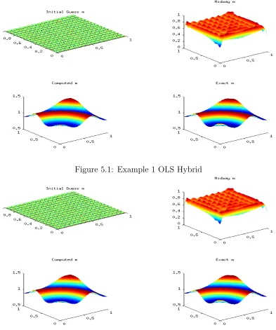
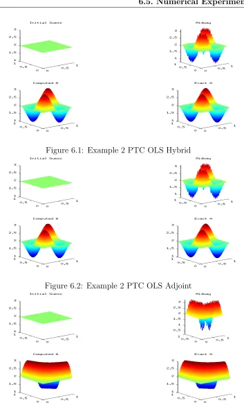
[image:45.612.108.501.208.679.2]The results reported in this section are done so to test the feasibility of the Second Order Adjoint method and the Hybrid method of Hessian computation. We use a second order technique to solve and compare these two methods.
Figure 5.1: Example 1 OLS Hybrid
35 5.2. Computations using OLS
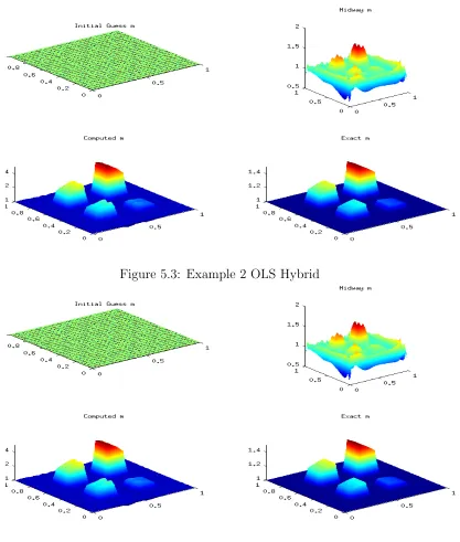
Figure 5.3: Example 2 OLS Hybrid
Figure 5.4: Example 2 OLS Adjoint
36 5.3. Heavy Ball with Friction Method
Method ε Iters Time (s) Error
1 OLS-H 10−6 15 45.3 4.68·10−3 OLS-A 10−6 15 87.9 4.68·10−3
2 OLS-H 10−11 44 1234.4 4.37·10−3
OLS-A 10−11 44 2571.5 4.37·10−3
5.3
Heavy Ball with Friction Method
Here we will report the results comparing the continuous newton-type method, and the HBF method.
5.3.1
Computations using MOLS
We report the results recovered using the MOLS functional for the Elasticity problem. We also report the parameters used, as well as the time, error and other qualitative variables and parameters involved in each example.
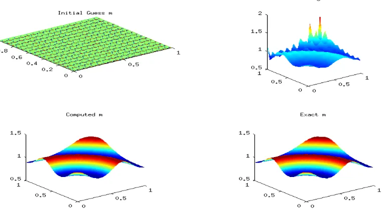
[image:47.612.116.497.379.596.2]For the continuous gradient method we have;
37 5.3. Heavy Ball with Friction Method
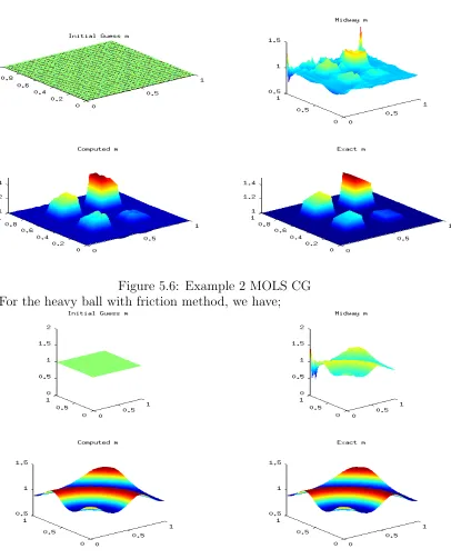
Figure 5.6: Example 2 MOLS CG For the heavy ball with friction method, we have;
38 5.3. Heavy Ball with Friction Method
Figure 5.8: Example 2 MOLS HB
Table 5.2: MOLS Numerical Results
Method HC MC GC ε α β Time (s) Iters λmin
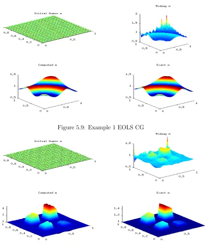
1 CG 13 0 0 10−6 - - 21.6 13 .1044
HB 9 0 0 10−6 2.02 1.02 13.8 9 .0985
2 CG 13 0 0 10−6 - - 182.0 13 .0486
HB 11 0 0 10−6 2.02 1.02 133.9 11 .0486
For example 1, the L2 Error recorded for both methods was 3.84·10−4. The
error for example 2, was 6.42·10−3.
5.3.2
Computations using EOLS
We report the results recovered using the EOLS scheme. We report the time, error, and other qualitative variables and parameters involved in each example
39 5.3. Heavy Ball with Friction Method
Figure 5.9: Example 1 EOLS CG
40 5.3. Heavy Ball with Friction Method
Figure 5.11: Example 1 EOLS HB
Figure 5.12: Example 2 EOLS HB
41 5.3. Heavy Ball with Friction Method
Method HC MC GC ε α β Time (s) Iters λmin
1 CG 13 0 0 10−6 - - 20.7 13 .1044
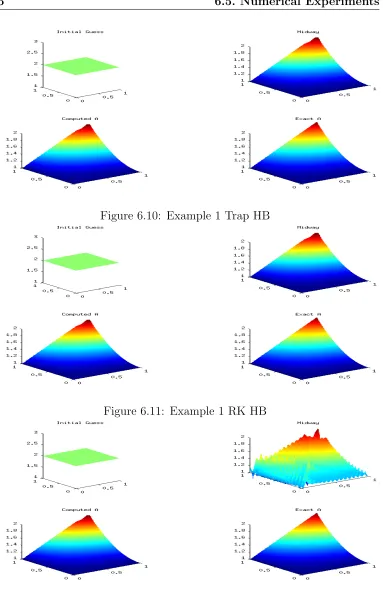
HB 9 0 0 10−6 2.02 1.02 14.1 9 .0985
2 CG 13 0 0 10−6 - - 183.3 13 .0486
HB 11 0 0 10−6 2.02 1.02 134.4 11 .0486
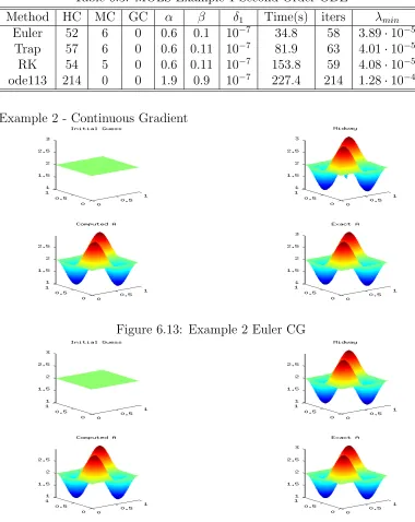
For example 1, the L2 Error recorded for both methods was 3.84·10−4. The
error for example 2, was 6.42·10−3
5.3.3
Computations using Equation Error
We report the results obtained from the use of the EE functional for the elasticity problem. We also report the time, error, and other qualitative variables and parameters involved in each example
For the continuous gradient method we have;
42 5.3. Heavy Ball with Friction Method
Figure 5.14: Example 2 EE CG For the heavy ball with friction method, we have;
43 5.4. Choice of Parameters for HBF
Figure 5.16: Example 2 EE HB
Table 5.4: EE Numerical Results
Method HC MC GC ε α β Time (s) Iters λmin
1 CG 6 0 0 10−6 - - 1.0 6 .165
HB 5 0 0 10−6 2.02 1.02 1.0 5 .165
2 CG 6 0 0 10−6 - - 3.0 6 .0917
HB 5 0 0 10−6 2.02 1.02 2.0 5 .0917
For example 1, the L2 Error recorded for both methods was 5.27·10−5. The
error for example 2, was 7.82·10−5
5.4
Choice of Parameters for HBF
The choice of the parameters α, andβ are very important when it comes to the number of iterations that the HBF method requires for convergence. It is important to maintain accuracy, and the choice of these parameters tend not to alter this as long as they are within reason. The table below is an example showing different choices of parameters and how they affect the number of iterations required to reach a certain level of accuracy.
44 5.4. Choice of Parameters for HBF
Table 5.5: Effect of Parameter Choice in Heavy Ball method
α β Iters Time (s)
2 2 1000 28.2
2.03 1.03 7 1.05
2.02 1.02 5 1.01
2 1 7 1.07
1 1 2557 88.2
0.6 0.1 56 2.64
0.1 0.1 10000 335.4*
0.4 0.06 73 3.74
* - This example was unable to reach required accuracy in 10000 iterations.
In all of these trial, the same level of accuracy is maintained, with the L2
Error being 5.27·10−5. As we can see the choice of these parameters α,
Chapter 6
Performance of Differential
Equations Based Solvers for
Noisy Data
6.1
Motivation
All of the optimization schemes utilized in this thesis work require data. This data is acquired through measurements made by machines that are prone to errors. This suggests that the data would be subject to a level of noise. As a result, the methods proposed need to be able to handle noise appropriately.
6.2
Objective and Approach
The purpose of this chapter is to compare different differential equation solvers, optimization techniques, and objective functionals. We consider the scalar problem because of its simplicity. It is computationally inexpensive compared to the elasticity problem. The differential equation techniques being considered include:
1. Euler’s Method
2. Trapezoidal Method
3. Runge Kutta Method
4. MATLAB’s ode113 solver
Figure

Related documents