analysis
.
White Rose Research Online URL for this paper:
http://eprints.whiterose.ac.uk/80732/
Article:
Zhao, Y, Kim, J and Filippone, M (2013) Aggregation algorithm towards large-scale
Boolean network analysis. IEEE Transactions on Automatic Control, 58 (8). 8. 1976 - 1985.
ISSN 0018-9286
https://doi.org/10.1109/TAC.2013.2251819
[email protected] https://eprints.whiterose.ac.uk/ Reuse
Unless indicated otherwise, fulltext items are protected by copyright with all rights reserved. The copyright exception in section 29 of the Copyright, Designs and Patents Act 1988 allows the making of a single copy solely for the purpose of non-commercial research or private study within the limits of fair dealing. The publisher or other rights-holder may allow further reproduction and re-use of this version - refer to the White Rose Research Online record for this item. Where records identify the publisher as the copyright holder, users can verify any specific terms of use on the publisher’s website.
Takedown
If you consider content in White Rose Research Online to be in breach of UK law, please notify us by
IEEE TRANSACTIONS ON AUTOMATIC CONTROL, VOL. XX, NO. XX, XXXX 201X 1
Aggregation Algorithm towards Large-Scale
Boolean Network Analysis
Yin Zhao,
Student Member, IEEE,
Jongrae Kim,
Member, IEEE,
and Maurizio Filippone,
Member, IEEE
Abstract—The analysis of large-scale Boolean network dynam-ics is of great importance in understanding complex phenomena where systems are characterized by a large number of compo-nents. The computational cost to reveal the number of attractors and the period of each attractor increases exponentially as the number of nodes in the networks increases. This paper presents an efficient algorithm to find attractors for medium to large scale networks. This is achieved by analyzing subnetworks within the network in a way that allows to reveal the attractors of the full network with little computational cost. In particular, for each subnetwork modeled as a Boolean control network, the input-state cycles are found and they are composed to reveal the attractors of the full network. The proposed algorithm reduces the computational cost significantly, especially in finding attractors of short period, or any periods if the aggregation network is acyclic. Also, this paper shows that finding the best acyclic aggregation is equivalent to finding the strongly connected components of the network graph. Finally, the efficiency of the algorithm is demonstrated on two biological systems, namely a T-cell receptor network and an early flower development network.
Index Terms—Boolean network, attractor, graph aggregation, acyclic aggregation
I. INTRODUCTION
M
ANY mathematical models have been proposed in the literature to study biological networks, including ge-netic regulatory networks [1].Boolean networkshave attracted particular interest because of their simplicity and potential to model a large number of nodes in the network. Boolean networks were first proposed by Kauffman [2] to model genetic regulatory networks. In this framework, each gene is assumed to have two levels, either active (on, true or 1) or inactive (off, false or 0), and to be affected by several other genes and/or by itself. Besides the genetic regulatory networks, Boolean networks can be also used to model other biological interactions, such as biomolecular signaling pathways [3]. Although Boolean networks are not as detailed as continuous models given in the form of differential equations [4], they have been widely and successfully used in Systems Biology [5]–[7]. Unlike continuous models that usually involve several parameters, which are difficult or even impossible to beY. Zhao is with the Key Laboratory of Systems & Control, Insti-tute of Systems Science, Academy of Mathematics & Systems Science, Chinese Academy of Sciences, Beijing 100190, P. R. China. E-mail: [email protected]
J. Kim is with the Division of Biomedical Engineering, University of Glasgow, Glasgow G12 8QQ, UK. E-mail: [email protected]
M. Filippone is with the School of Computing Science, University of Glas-gow, Glasgow G12 8QQ, UK. E-mail: [email protected]
Manuscript received August 14, 2012; revised December 15, 2012 & January 25, 2013;
x1 x2
[image:2.612.399.477.177.264.2]x3
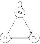
Fig. 1. An example of a network Graph comprising three nodes.
estimated or inferred, Boolean networks are parameter free models. One of the main problems in Boolean network model-ing for biological or any physical dynamics is the identification of the update rules using observed data [8], [9]. Once these are obtained, similarly to the analysis of continuous systems, the dynamical properties of Boolean networks are analyzed by finding steady-states, attractors, size of the basin of attraction to each attractor, etc. Steady-states and attractors in particular are the most important characteristics when they are related to some specific physiological responses in biological networks [2], [10]–[13].
The interactions of genes or some biomolecular species are presented by logical functions as exemplified in Fig. 1 and its corresponding logical equations (1). The network graph in Fig. 1, shows an example of the interactions between the three nodes x1,x2, andx3; a directed edge from node xi to
xj means that the state (active or inactive) ofxj at timet+ 1
is affected by the state ofxi at timet.
As an example, consider the following updating rules among all possible functions corresponding to Fig. 1:
x1(t+ 1) =f1[x2(t), x3(t)] =x2(t)∧x3(t),
x2(t+ 1) =f2[x1(t), x3(t)] =x1(t)∨x3(t),
x3(t+ 1) =f3[x3(t)] =¬x3(t),
(1)
where∧,∨,¬denote “AND”, “OR”, and “NOT” respectively. The nodes in a network graph having no in-degrees, i.e., nodes that are not affected by others and/or themselves, can be interpreted as input nodes, while the nodes having no out-degrees can be interpreted as output nodes. Boolean networks with input nodes are calledBoolean control networksand they form the building blocks that will be used in this paper to reveal attractors of larger networks. For example, considering onlyx1 andx2and ignoring the update rule for x3 in (1),x1
andx2in Fig. 1 can be defined as a Boolean control network,
where the dynamics of x1 and x2 are given by the first two
Boolean networks withnnodes have2nnumber of possible
states and it is proved that the computational complexity of Boolean network related problems of interest is NP-hard [14]. Even for small Boolean networks, e.g. n around 50 or 100, it is almost impossible to find all attractors, in general. A lot of effort has been devoted to the solution of this issue, at least partially. One way to find attractors is to choose some initial states wisely and simulate the dynamics for each initial condition [15]; however, the global dynamics can be hardly revealed by this method. In [11], a probabilistic method is developed by choosing initial states randomly to find a certain percentage of steady states with a given confidence level. In our previous work [16], Boolean networks are divided into several groups and the input-output structure of each group approximates the global dynamics. However, only part of the nodes can be approximated and some information is lost.
The main motivation of the idea to use network aggregation in [16] is from [17], where the web is partitioned to reduce the computational cost in calculating page rank. Some aggregation methods are also discussed in [18], [19] and the references therein. In this work, we build upon the idea of aggregation of Boolean networks into several subnetworks, but instead of the approximation, the structure of the attractors of Boolean networks is accurately recovered by the composition of the input-state cycles of subnetworks.
The paper is organized as follows: section 2 describes the aggregation of Boolean networks; section 3 provides the method of revealing attractors of Boolean networks by composing the input-state cycles of subnetworks, and analyzes its computational complexity; section 4 presents a special aggregation structure called acyclic aggregation, for which the suggested algorithm is particularly efficient; the efficiency of the algorithm is demonstrated in section 5 using T-cell receptor network and an early flower development network; finally, section 6 presents the conclusion.
II. AGGREGATION OFBOOLEANNETWORKS Consider the following Boolean network:
x1(t+ 1) =f1[x1(t), x2(t), . . . , xn(t)],
x2(t+ 1) =f2[x1(t), x2(t), . . . , xn(t)],
· · ·,
xn(t+ 1) =fn[x1(t), x2(t), . . . , xn(t)],
(2)
wherexi(t)for i= 1, 2, . . . , n denotes the state of node xi
at time t that can be either0 for inactive or1for active. The nodes can be partitioned intos-number of blocks as follows:
X ={x1, x2, . . . , xn}=X1∪ X2∪. . .∪ Xs,
whereXi is a proper subset ofX,Xi∩ Xj is empty fori6=j,
Xi={xi1, xi2, . . . , xini},niis the number of nodes in thei
-th block, andxij, thej-th node in thei-th block, is equal toxk
for ak∈ {1,2, . . . , n}. We call this partition anaggregation of the Boolean network.
Each blockXihas incoming edges from outside of the block
and some outgoing edges to the outside. The source nodes of these edges can be interpreted as inputs and outputs for each block. Denote the set of inputs and outputs of the blockXi as
x2
x1
x3
x4
x5
x7
x8
x6
x9 Σ1
Σ2
[image:3.612.336.535.55.244.2]Σ3
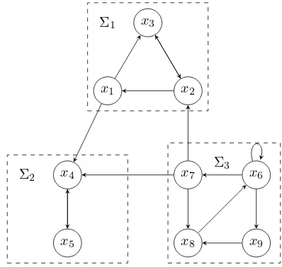
Fig. 2. An example of aggregation of a network comprising nine nodes into three Boolean control networks.
Ui = {ui1, ui2, . . . , uimi} and Yi = {yi1, yi2, . . . , yipi},
respectively, and the set of all source nodes, whose edges cut by the partition, asC={xc1, xc2, . . . , xcp}. Note thatUi
and/or Yi could be empty set, i.e., there are no input and/or
output to and from thei-th block.
Remark 2.1:
1) yiq in Yi is a node in Xi and uil in Ui is a node in
another block, i.e.,
Yi⊂ Xi⊂ X andUi∩ Xi=∅.
2) Each xcj ∈ C belongs to only one block (the output of
a specific block), but could be the input of several other blocks. Hence,
C=
s
[
i=1 Yi=
s
[
i=1 Ui,
Yi∩ Yj=∅, i6=j,
p=
s
X
i=1
pi≤ s
X
i=1
mi.
Then, the subnetwork Σi, with nodes inXi and inputs in
Ui, is a Boolean control network given by
Σi: xij(t+ 1) =fij[xi1(t), xi2(t), . . . , xini(t), ui1(t), ui2(t), . . . , uimi(t)],
(3)
for i= 1,2, . . . , sandj= 1, 2, . . . , ni.
ZHAOet al.: AGGREGATION ALGORITHM TOWARDS LARGE-SCALE BOOLEAN NETWORK ANALYSIS 3
2. Assume its dynamics is described as
x1(t+ 1) =x2(t)
x2(t+ 1) =x3(t)∧x7(t)
x3(t+ 1) =x1(t)↔x2(t)
x4(t+ 1) = (x1(t)∨x5(t))→x7(t)
x5(t+ 1) =¬x4(t)
x6(t+ 1) =x6(t)¯∨x8(t)
x7(t+ 1) =x6(t)
x8(t+ 1) =x7(t)∨x9(t)
x9(t+ 1) =¬x6(t),
(4)
where ↔, →, and ∨¯ denote “EQUIVALENCE”, “IMPLI-CATION”, and “EXCLUSIVE-OR” operations respectively. Consider the aggregation into 3 blocks as shown in Fig 2,
{x1, x2, x3} ∈ X1, {x4, x5} ∈ X2, {x6, x7, x8, x9} ∈ X3.
Now the inputs and outputs of each subsystem are
U1={u11=x7}, U2={u21=x1, u22=x7}, U3=∅, Y1={y11=x1}, Y2=∅, Y3={y31=x7},
C={xc1 =x1, xc2=x7}.
Hence, there are three subnetworks
Σ1:
x1(t+ 1) =x2(t)
x2(t+ 1) =x3(t)∧u11(t)
x3(t+ 1) =x1(t)↔x2(t);
Σ2:
(
x4(t+ 1) = (u21(t)∨x5(t))→u22(t)
x5(t+ 1) =¬x4(t);
Σ3:
x6(t+ 1) =x6(t)¯∨x8(t)
x7(t+ 1) =x6(t)
x8(t+ 1) =x7(t)∨x9(t)
x9(t+ 1) =¬x6(t).
Note that the aggregation shown in Example 2.2 is not unique but there are many other different configurations. How to construct the best aggregation of the network to minimize the cost to find attractors will be discussed in section 4.
III. REVEALINGATTRACTORS OF THEWHOLENETWORK
Finding attractors is one of the main problems in analyzing Boolean networks. Attractors are defined as follows:
Definition 3.1:
1) Consider the Boolean network given by (2). Its State Transition Graph is defined as a directed graph
{Dn,E}, whereD:={0,1} and
E ={a→b|a, b∈ Dn, b=f(a)},
wheref = [f1, f2, . . . , fn]T.
2) A periodic path of the state transition graph is called an attractor of a Boolean network (2). An attractor with period1is also called a fixed point. Denote an attractor as
{a1→a2→. . .→aℓ→a1},
000 001 010 101
111 110 011 100
Fig. 3. State transition graph for (1), where states are ordered as(x1x2x3)
01 10
[image:4.612.68.264.358.493.2]11 00
Fig. 4. State transition graph for Boolean control network (1), where states are ordered as(x1x2)and the controlu=x3is indicated by the solid arrow foru= 1, or by the dashed arrow foru= 0.
where ai ∈ Dn, i = 1, 2, . . . , ℓ, and ℓ is the period
or the length of the attractor. Attractors are also called cycles.
Example 3.2: Fig. 3 shows the state transition graph of Boolean network (1), and there are two attractors as follows:
{(0 0 1)→(0 1 0)→(0 0 1)},
{(1 1 0)→(0 1 1)→(1 1 0)}.
For a Boolean control network,
xi(t+ 1) =fi(x1(t), . . . , xn(t), u1(t), . . . , um(t)), (5)
for i= 1,2, . . . , n, we have a similar definition of attractors as follows:
Definition 3.3:
1) Consider the Boolean control network given by (5). Its State Transition Graph is defined as a directed graph
{Dn,E}, where
E={a→b|a, b∈ Dn,∃u∈ Dm, b=f(a, u)},
in which f = [f1, f2, . . . , fn]T.
2) A periodic path of the state transition graph is called a cycle.
Example 3.4:Fig. 4 shows the state transition graph, where
x3 is considered as the input in (1) (i.e., the edge from x3
to itself is ignored). As there is one input, each state in the state transition graph has two outgoing edges depending on the different value of the input. For example, the cycle {(00)→ (00)→(01)→(00)}in Fig. 4 is not an elementary cycle.
Input-state cycles of Boolean control networks need to be considered and they are defined by
Definition 3.5:
1) Consider the Boolean control network given by (5). Its Input-State Transition Graph is defined as a directed graph{Dn+m,E}, where
E=
(a, u)→(b, u′)
a, b∈ Dn, u, u′∈ Dm
, b=f(a, u) ,
in which f = [f1, f2, . . . , fn]T.
2) A periodic path of the input-state transition graph is called an input-state cycle.
3) A periodic path with no repeated state in one period of the input-state transition graph is called a elementary input-state cycle.
The definition implies that if there exits an u′ inDm such
that an edge (a, u) → (b, u′) exists, then edges (a, u) → (b, u′′)for allu′′inDmexist as well. For more details about
input-state cycles of Boolean control networks, refer to [21], where the input-state cycles are simply called cycles.
It is easy to divide an input-state cycle with repeated states into several elementary input-state cycles, and conversely, it is also easy to combine elementary input-state cycles into cycles. Thus, we can use the algorithm in [20] to find all elementary input-state cycles, and then obtain input-state cycles by com-bination of these elementary ones; or alternatively, we can use the method in [21] to find input-state cycles directly. Note that, the number of elementary input-state cycles is much less than the number of input-state cycles. In fact, the number of input-state cycles may be infinite if the length is not limited. However, later we will see that the input-state cycles longer than2n are meaningless.
The main problem is now how to reveal an attractor of the whole Boolean network (2) from the input-state cycles of the subnetworks (3). To this end, denote Ai as the set of
input-state cycles in Σi and define πi(·, j) : Dni+mi → D as the
projection of a state ainDni+mi onto the state ofx
j, where
xj ∈ Xi∪ Ui. In addition, define the projection Πi(·, j) of
an input-state cycle A ∈ Ai onto the periodic trajectory of
xj, where xj ∈ Xi∪ Ui, as follows: for a length-ℓinput-state
cycle,
A={a1→a2→ · · ·aℓ→a1}.
The projection,Πi(, j), is given by
Πi(A, j) :={πi(a1, j)→πi(a2, j)→ · · · →pii(aℓ, j)→πi(a1, j)}.
Note that the period of Πi(A, j) would be a divisor of ℓ.
For notational simplicity, Π(·, j) is used without indicating the domain of each projection if there is no ambiguity.
Then we define the composition of two input-state cycles from different subnetworks. Note that, hereafter, if a subnet-work has no input nodes, we use its attractors, or say cycles,
A1 0
1 0 0 1
0
0
1
0
0 1
0
A2 1 0 0
[image:5.612.355.517.59.196.2]1 0
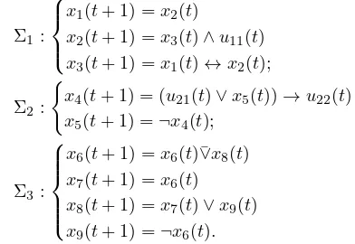
Fig. 5. An example of composition of two input-state cycles
instead of input-state cycles. Assume Σ1 and Σ2 are two
subnetworks, and
X1∪ U1={x1, . . . , xk1, xk1+1, . . . , xk1+k2}, X2∪ U2={x1, . . . , xk1, xk1+k2+1, . . . , xk},
where x1, x2, . . ., xk1 are the common components in two
subnetworks. If there are two input-state cycles for Σ1 and Σ2 with length,ℓ1 andℓ2, respectively, i.e.,
A1={a1→a2→ · · · →aℓ1 →a1} ∈ A1, A2={b1→b2→ · · · →bℓ2→b1} ∈ A2,
and Π(A1, j) = Π(A2, j) for j = 1,2, . . . , k1, then the
composition ofA1andA2, i.e.A1×A2, is defined as follows:
1) RepeatA1andA2 to length-ℓperiodic pathsA˜1andA˜2
whereℓ=lcm(ℓ1, ℓ2) ˜
A1={a˜1→˜a2→ · · · →˜aℓ→˜a1}, ˜
A2={˜b1→˜b2→ · · · →˜bℓ→˜b1},
where lcm(·,·) is the least common multiple of the arguments.
2) Adjust the order of states in A˜1 and A˜2 by circular
permutation in order to make Π( ˜A1, j) and Π( ˜A2, j)
equal to each other for j= 1,2, . . . , k1.
3) A1×A2 is given by
A1×A2=
nh ˜
a1, π(˜b1, p), π(˜b1, p+ 1), . . . , π(˜b1, k)
i
→h˜a2, π(˜b2, p), π(˜b2, p+ 1), . . . , π(˜b2, k)
i
→
· · · →h˜aℓ, π(˜bℓ, p), π(˜bℓ, p+ 1), . . . , π(˜bℓ, k) i
→ ha˜1, π(˜b1, p), π(˜b1, p+ 1), . . . , π(˜b1, k)
io ,
wherep=k1+k2+ 1. This is akin to the mechanism
of two gears rotating together, as illustrated in Fig. 5. The following example demonstrates the composition pro-cedures:
Example 3.6:Consider two input-state cycles
A1={(0 0 1)→(1 0 1)→(0 1 1)→(1 1 0)→(0 0 1)}
ZHAOet al.: AGGREGATION ALGORITHM TOWARDS LARGE-SCALE BOOLEAN NETWORK ANALYSIS 5
where the states in A1 are ordered as (x1, x2, x3), and the
states inA2 are ordered as(x1, x4). Their projections ontox1
are
Π(A1,1) ={0→1→0→1→0}={0→1→0} Π(A2,1) ={1→0→1},
thus,Π(A1,1) = Π(A2,1). We can compose them.
1) Repeat A1 andA2 to length-4 periodic paths ˜
A1={(0 0 1)→(1 0 1)→(0 1 1) →(1 1 0)→(0 0 1)} ˜
A2={(1 1)→(0 0)→(1 1)→(0 0)→(1 1)}.
2) The projections of A˜1 andA˜2 ontox1 are
Π( ˜A1,1) ={0→1→0→1→0}={0→1→0} Π( ˜A2,1) ={1→0→1→0→1}={1→0→1}.
To make them equal to each other, reorder of the states inA˜2 as
˜
A2={(0 0)→(1 1)→(0 0)→(1 1)→(0 0)}.
3) The composition is given by
A1×A2={(0 0 1π[(0,0),4])→(1 0 1π[(1,1),4]) →(0 1 1π[(0,0),4])→(1 1 0π[(1,1),4]) →(0 0 1π[(0,0),4])}
={(0 0 1 0)→(1 0 1 1)→(0 1 1 0) →(1 1 0 1)→(0 0 1 0)}.
Finally, we are ready to present an algorithm to recover the attractors of the whole network from its subnetworks. It is assumed that Boolean network graphs considered are at least weakly connected, i.e., there is always a path between any two nodes if the direction of the edges is ignored. This excludes networks with isolated multiple groups, where each isolated group can be analyzed one by one using the proposed algorithm in the following, if needed.
Algorithm 3.7: The attractors of the Boolean network (2) can be obtained by applying the following steps:
1) Partition the network graph to s-number of blocks {X1,X2, . . . ,Xs}, and reorder them to
{Xi1,Xi2, . . . ,Xis} such that the corresponding Xiα
andUiα for2≤α≤s satisfy
α−1
[
β=1
Xiβ∪ Uiβ
∩(Xiα∪ Uiα)6=∅, (6)
i.e., each block is connected to the union of all blocks in front in the order by at least one edge.
2) For each subnetwork Σi, find all elementary input-state
cycles, and then combine them to obtain all input-state cycles ofΣi with the length of period less than or equal
to2n. Denote the set of all input-state cycles asA i, for
i= 1,2, . . . , s.
3) Find an attractor of Boolean network (2) by composing the input-state cycles of subnetworks as follows:
(((Ai1×Ai2)×Ai3)× · · ·)×Ais, (7)
whereAiα belongs toAiα, and{Aiα|α= 1,2, . . . , s}
must satisfy the following for all xck inCandα,β in {1,2, . . . , s}:
Π(Aα, ck) = Π(Aβ, ck) (8)
wheneverxckis an element of (Xα∪ Uα)∩(Xβ∪ Uβ).
Theorem 3.8:Consider the Boolean network (2), partitioned to subnetworks (3), where its network graph is assumed to be weakly connected, i.e. no isolated nodes in the network graph. The composition given by (7) is an attractor of Boolean network (2), and all attractors of the Boolean network (2) can be recovered using the above algorithm.
Proof.Firstly, as the network graph is weakly connected, for any aggregation, we can always find two subnetworksΣi1 and
Σi2 such that(Xi1∪ Ui1)∩(Xi2∪ Ui2)is non-empty, i.e.,Σi1
andΣi2 satisfying the condition (6) forα= 2. Then, we can
find further Σi3 such that (6) holds for α= 3 because of the
weak connectivity of the network. These procedures, dividing and ordering the subnetworks to the index, {i1, i2, . . . , iα},
such that (6) holds, are repeated till α=s. Each edge of an input-state cycleAik satisfies the dynamics ofΣik in (3). (8)
ensures that the states of overlapping nodes of the input-state cycles in (7) are equal to each other. Therefore, the edges of the composition (7), satisfy the overall dynamics (2), and (7) is an attractor of the Boolean network (2).
Conversely, for any attractorAof the Boolean network (2), by projecting it onto the nodes in Xik ∪ Uik, for k =
1, 2, . . . , s, an input-state cycles Aik, is obtained and (8)
holds, and the composition of Aik’s is equal to A. Hence,
all the attractors of the Boolean network (2), can be revealed
by (7).
As the attractors of the Boolean network (2), cannot be longer than 2n, their projections onto each subnetwork are
shorter than or equal to2n as well. Hence, finding input-state
cycles, whose length is longer than 2n, is not necessary.
Complexity Analysis: The proposed algorithm has four main parts as follows:
P1. Aggregation of the Boolean network
P2. Finding all elementary input-state cycles for each sub-network
P3. Combine the elementary input-state cycles to input-state cycles
P4. Compose the input-state cycles to attractors of the whole network.
Comparing to P2, the complexity of P1 is negligible as the computational cost increases polynomially with the size of the networks. For example, to calculate the eigenvectors of the Laplacian matrix of network graph, whose size isn×n, the complexity is O(n3)
if we use a spectral partitioning method such as min-cut aggregation [18] or max-modularity aggregation [19]. For P2, on the other hand, the fastest algorithm for finding all the elementary cycles of general graph is Johnson’s algorithm [20], [22] and its complexity is
O((n+e)(c+ 1)), where n, e, c are the numbers of nodes, edges, and elementary cycles respectively. Thus, for each subnetwork, the complexity to complete P2 is in the order of O((2mi+ni+ 22mi+ni)( ˜N
TABLE I
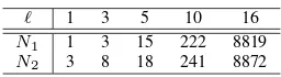
NUMBER OF INPUT-STATE CYCLES(Ni),WHERE THE PERIOD IS LESS THAN OR EQUAL TOℓ
ℓ 1 3 5 10 16
N1 1 3 15 222 8819
N2 3 8 18 241 8872
of elementary input-state cycles ofΣi, and it is bounded above
by O(s22mα+nαN˜
α), where α=argmaxi{22mi+niN˜i}. The
complexity of P3 together with P4 is no more thanO((Nβℓ¯)s),
whereβ =argmaxi{Ni},ℓ¯is the length of the longest
input-state cycles, andNiis the number of input-state cycles shorter
than or equal to 2n. Note that unlike the elementary
input-state cycles, input-input-state cycles in Boolean control networks may have repeated states in general, thus Ni may be much
greater than N˜i.
The total number of states of Boolean networks with n -nodes is 2n and the transition from each state to an updated
state is unique. Thus, finding the cycles of whole Boolean networks directly requires computations in order 2n.
Com-paring O(s22mα+nαN˜
α+ (Nβℓ¯)s)withO(2n), the proposed
method will be very efficient if the size of each subnetwork is small enough and Ni’s are not too big. If not, the algorithm
requires more computations than the one of the brute force computation. This is an inherent difficulty of solving NP-hard problems. For the Boolean network whose network graph is sparse, on the other hand, if it is possible to set a reasonable size M(≪ n), and partition the network such that subnetwork size, 2mi+ni, is less than or equal toM,
then the computational reduction will be significant. Note that the sparse network structure is quite common in biological networks [23], [24].
Another very important issue is the number of input-state cycles Ni for each subnetworks. The number of input-state
cycles of Boolean control networks may be very large for long period attractors. However, we may be less interested in longer attractors as most of biologically and physically meaningful dynamics are related to the short period attractors including fixed points. If we are to find attractors with the length of period less than or equal to a fixed number T, Ni
would not be very large. If T = 1, i.e. finding fixed points, the proposed algorithm yields the results extremely quickly. The mean maximum attractor length of Boolean networks is shown to be proportional to√nin [1], thus it is reasonable to set T ≤√n, although in some cases there may be attractors longer than √n.
In the following example, the strength of the proposed algorithm and the computational issues are highlighted.
Example 3.9: Consider a Boolean network whose network graph is partitioned as shown in Fig. 6 and its dynamics is given by
x1(t+ 1) =x2(t)∨x3(t)
x2(t+ 1) =¬x1(t)
x3(t+ 1) =x4(t)
x4(t+ 1) =x2(t)∧x3(t).
x1 x2
x3 x4
Σ1
[image:7.612.110.238.91.126.2]Σ2
Fig. 6. Boolean network of example 3.9
Ni, the number of input-state cycles for each subnetwork,
whose length is less than or equal to ℓ, is shown in Table I. Even in this simple example, the number of input-state cycles, not the number of elementary input-state cycles, is huge. Thus, trying to find all attractors using the proposed algorithm requires more computation than the brute-force algorithm. The network has in fact only one attractor as follows:
{(1100)→(1000)→(0000)→(0100)→(1100)},
and it is composed by
A1={(110)→(100)→(000)→(010)→(110)},
where the state is arranged in(x1, x2, x3), and
A2={(100)→(100)→(000)→(000)→(100))},
where the state is arranged in(x2, x3, x4), with their
projec-tions ontox2 andx3 satisfying:
Π(A1,2) = Π(A2,2) ={1→1→0→0→1}, Π(A1,3) = Π(A2,3) ={0→0}.
In order to find this attractor through the proposed algorithm the computational cost is much larger than the brute-force algorithm. However, if we only want to find fixed points, i.e.
T = 1, fixed points for both subnetworks are found as follows:
A11={(101)→(101)}
A21={(111)→(111)}, A22={(100)→(100)},
A23={(000)→(000)},
where Aij is j-th input-state cycle of i-th subnetwork. It is
immediately concluded that there are no fixed points as Aij
cannot be composed and these can be calculated very quickly.
IV. ACYCLICAGGREGATION
There could be a large number of input-state cycles with long periods in each subnetwork if a Boolean network is divided into several subnetworks as demonstrated in Example 3.9. As already pointed out earlier, the proposed algorithm is only efficient to find short period attractors. However, the following example shows that we can also find efficiently all the attractors for Boolean networks with a special structure.
Example 4.1:Recall Example 2.2. AsΣ3 has no input, it is
a Boolean network itself rather than a Boolean control network and it has a far less number of attractors compared to Boolean control networks in general. It can be easily seen that there is only one attractor ofΣ3 and it is as follows:
ZHAOet al.: AGGREGATION ALGORITHM TOWARDS LARGE-SCALE BOOLEAN NETWORK ANALYSIS 7
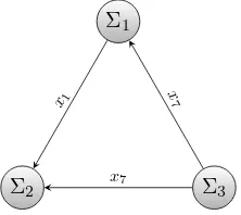
Σ3 Σ1
Σ2
x1 x7
[image:8.612.120.231.57.156.2]x7
Fig. 7. Example of aggregation graph corresponding to example 4.1
where the state is ordered as (x6, x7, x8, x9). The projection
onto its output x7is given by
Π(A3,7) ={0→1→0}.
The attractors of Σ1 to be composed withA3 must have the
same projection onto its inputs x7. Thus, the input sequence
toΣ1 can be fixed to {0,1,0,1, . . .}.Σ1 becomes a periodic
time-varying Boolean network with the fixed periodic input from Σ3. As the input is fixed, the number of possible
input-state cycles of the Boolean control network Σ1 is much less
than the one with free input. It is now easy to obtain all input-state cycles ofΣ1, with the fixed input sequence. There is only
one as follows:
A1={(1001)→(0000)→(0011)→(0110)→(1001)},
where the state is ordered as(x1, x2, x3, x7). Finally, asx1and
x7 are inputs toΣ2, we now fix the input sequence,(x1, x7),
toΣ2 as follows:
{(11),(00),(01),(00),(11),(00),(01),(00),· · · }.
The corresponding input-state cycles of Σ2 are obtained as
follows:
A21={(1101)→(0100)→(0101)→(0100)→(1101)},
A22={(1001)→(0110)→(0001)→(0110)→(1001)},
where the state is ordered as (x1, x4, x5, x7).
Hence, all attractors of the whole network are found by
(A3×A1)×A21, and(A3×A1)×A22.
Consider the network graph of a Boolean network shown in Fig. 7, where each block Σi represents a super node, and
call it aggregation graph. If there are no periodic path in the aggregation graph, which is the case of Example 4.1, we call this aggregation anacyclic aggregation. In this case, there exist several root blocks, which have no input, i.e. they are Boolean networks. By projecting the outputs from the root blocks onto their child blocks, the child blocks are turned into periodic time-varying Boolean networks. Repeat these procedures until all blocks can be driven by the outputs from their parent blocks. In these procedures, there is no need to find all input-state cycles in each subnetwork and the computational demand decreases significantly. The only remaining question is how to find an acyclic aggregation if there exists any for a given network structure. To this end, we introduce some classical concepts in graph theory in the following:
Definition 4.2:
1) G ={X, E} is a directed network graph, where X is the set of nodes and E is the set of directed edges.
xi→xj∈E, ifxi andxj are elements ofX, and there
exists an edge starts at xi and ends atxj.
2) The directed graph G is called strongly connected, if for any xi, xj ∈ X there is a pathxi →xk1 →xk2 → . . .→xkp→xj from xi toxj.
3) G′ ={X′, E′} is called a subgraph of G, if X′ ⊂ X, and for all xi, xj ∈ X′, xi → xj ∈ E implies xi →
xj∈E′.
4) The subgraph G′ ={X′, E′} of Gis called a strongly connected component, if it is a maximal strongly con-nected subgraph, i.e. adding any nodes that are not elements ofX′and the corresponding edges toE′makes the obtaining subgraph being not strongly connected. Note that a single node can also be a strongly connected component.
5) For two aggregations of G, P1 ={X11,X12, . . . ,X1p},
P2 = {X21,X22, . . . ,X2q},P1 is said to be finer than
P2, if for anyX1i ∈P1, there exists anX2j ∈P2 such
that X1i⊂ X2j.
It is easy to see that any two strongly connected components of a directed graph are disjoint. Thus, strongly connected components form an aggregation of the graph and we call it graph of strongly connected components. The following two lemmas are also classical results from graph theory. They show the relationship between strongly connected components and acyclic aggregation.
Lemma 4.3: A strongly connected graph does not have acyclic aggregations.
Proof.For any two network partitions,G1andG2, of any
ag-gregation of a strongly connected graph,G, and two arbitrary nodes,a∈G1 andb∈G2, there are paths fromatob, andb
toaby the definition of strongly connected graph. Then, the paths form a cycle between G1 andG2. Hence, the strongly
connected graph cannot be acyclic.
Lemma 4.4:The graph of strongly connected components of a directed graphG, is acyclic.
Proof. If the graph of strongly connected components of G
is not acyclic, there are k strongly connected components,
G1, G2, . . . , Gk, which form a cycle, where k >1. For any
a ∈ Gi, b ∈ Gj, i 6= j, i, j = 1,2, . . . , k, there exists a
path from a to b and a path from b to a and ∪ki=1Gi turns
out to be strongly connected. This contradicts the fact that the strongly connected components are maximally strongly
connected subgraphs.
Combining these two lemmas, the following is trivial: Corollary 4.5:The graph of strongly connected components of a directed graph is finer than any other acyclic aggregation. There are many existing efficient algorithms for finding strongly connected components, for example, Tarjan’s algo-rithm [25], which can be used to find the acyclic aggregation of the network graph of a Boolean network.
CD45 CD4 T CRbind T CRlig
P AGCsk cCbl
F yn Lck
T CRphos Rlk ZAP −70
LAT phop Gads
SLP76
P LCgbind
Itk PLCgact
IP3
DAG Caplus
Calcin N F AT
P KCth RasGRP1
Grb2Sas
Ras
Raf SEK IKKbeta
IkB J N K
M EK
ERK J U N N F kB
Rsk F os
CREB CRE
[image:9.612.163.447.55.360.2]AP1
Fig. 8. Boolean network implementing a T-cell receptor model as presented in [26]
to be analyzed. The network graph of T-cell receptor kinetics is shown in Fig. 8, where the solid arrows with pointed heads represent activation, the dashed arrows with bar heads represent inhibition, the big bullets represent “AND”, and the boxes with more than one arrow pointed to them represent “OR”. For example, for P AGCsk, there is a dashed arrow from T CRbind and a solid arrow from F yn pointed to its box, thus its update rule is
P AGCsk(t+ 1) =¬T CRbind(t)∨F yn(t).
There are three external inputs, CD45,CD4, andT CRlig
and the inputs are fixed to (1, 1, 1) as [11] so that the analysis of the responses of T-cell receptor kinetics focuses on a specific physiological input situation. The assumption of the inputs being constant during the analysis is based on the fact that for most biological networks external inputs cannot change fast and frequently enough during their dynamic responses. Note that, however, any periodic or constant ex-ternal input scenarios can be analyzed without any significant increasing computational demand. Second, it is easy to see that the following nodes compose a strongly connected component having no input, i.e.X1 is a root block,
X1={T CRbind, P AGCsk, Lck, F yn, cCbl,
T CRphos, ZAP −70}.
The attractors ofΣ1corresponding toX1can be easily found,
for example, using the semi-tensor approach toolbox, as it is a Boolean network with only7nodes. Using a PC with Dual-Core2.5GHz CPU,8G RAM, it takes only0.0983s to find all
(two) attractors as follows:
A11={(1101010)→(1101010)},
A12={(1111010)→(1101011)→(1101110)→ (0101010)→(1100010)→(1001000)→ (1111010)},
where the states are ordered as (T CRbind, P AGCsk, Lck, F yn, cCbI, T CRphos, ZAP −70). For the rest of nodes, each node is now considered as an individual block, i.e., a subgraph with one node. For each single-node block, which does not have any self-feedback, one periodic input will drive only one attractor of the block Thus, each attractor of Σ1
can generate only one attractor in the whole network. It takes only0.0278s to calculate two attractors of the whole network. Their projection onto the outputs of the T-cell receptor are as follows:
{(0100)→(0100)}
{(0100)→(0100)→(0100)→ (0100)→(0101)→(0100)},
where the states are ordered as (N F AT, N F kB, AP1, CRE).
Hence, it takes a total 0.126s only to find all attractors in the T-cell receptor network. This is remarkable compared to other approaches to find all attractors in such a large Boolean networks. Given that the total number of states is 237
ZHAOet al.: AGGREGATION ALGORITHM TOWARDS LARGE-SCALE BOOLEAN NETWORK ANALYSIS 9
the semi-tensor product approach [12] or random initial state evaluation [11]. In [11], the authors applied their algorithms to the asynchronous case of T-cell receptor to compare the running times: 20.7 minutes using Genysis’s algorithm [27],
11.3s and 2.1s using their algorithm to find 90% percent steady states with 90% confidence and 80% percent steady states with 80% confidence respectively. However, only very few (far less than 1%) of the states in state space need to be considered using their algorithm applied to asynchronous Boolean networks. Their algorithm can also be applied to synchronous Boolean networks, but for synchronous Boolean networks no states can be excluded a priori, thus the total237
number of states in the state space of T-cell receptor network must be considered and it would take at least several hours to perform all the calculations. Moreover, the computation time increases drastically from hours to years by adding two or more nodes to the network.
The other 7 different external input combination cases are analyzed and the corresponding outputs are summarized in Table II, where inputs are ordered as(CD45, CD4, T CRlig)
and outputs are ordered as (N F AT, N F kB, AP1, CRE). The results shown in the table imply that the T-cell receptor response is rather robust, as most input combinations cannot change its steady states if the inputs remain constant for a sufficient amount of time.
Note that the T-Cell receptor model contains only one strongly connected component with more than one node; all the rest are single-node blocks. This structure of network graph is ideal for our algorithm in terms of computational efficiency. In order to demonstrate the performance of the algorithm on a less trivial example, an early flower development network is used [28]. Its network graph comprises 24 nodes (excluding the input nodes) and turns out to have also acyclic aggregation. It has two strongly connected components with more than one node: one has 8 nodes and another has 4 nodes. Using the proposed algorithm, it takes only 0.176s to find all attractors (in fact there is only one), while it is impossible to use a standard PC to analyze the attractors of this network using the semi-tensor product approach directly.
VI. CONCLUSION
In order to reduce the computational complexity in finding attractors of Boolean networks an aggregation algorithm is developed. The proposed algorithm is based on the idea of dividing the whole network into several subgraphs and of composing the attractors of the whole networks from the input-state cycles found in each subnetwork. The algorithm is shown to be more efficient than finding attractors directly from the whole network in the following scenarios: i) the network graph can be divided into a few subnetworks, whose sizes are small enough to be analyzed using some analytic methods, e.g., the semi-tensor approach, ii) short-period attractors are to be found, and/or iii) the aggregation graph is acyclic.
If a Boolean network is put into an acyclic aggregation by finding strongly connected components in the graph where all components are small enough (say, less than 20 nodes or so), the proposed algorithm finds all attractors of the Boolean
network very efficiently. On the other hand, if the network graph cannot be partitioned acyclically (i.e., the network graph is itself strongly connected), or some strongly connected com-ponents are too large, then large network comcom-ponents can be divided into smaller blocks using the min-cut criterion; short-period attractors can still be found with little computation using the proposed algorithm.
In many applications, some variables have more than two states, i.e. multi-valued logical networks or their update rules are functions of continuous variables, i.e., mixed-valued log-ical networks [13], [29]. For example, the state of genes and the concentration of proteins are quantified to more than two levels and simple PID controllers for engineering systems are implemented with logical decision algorithms. Generalization of the suggested algorithm to those cases will produce powerful tools to analyze various dynamical systems.
ACKNOWLEDGMENT
This research was initiated during J. Kim’s visiting to the Institute of Systems and Science, Chinese Academy of Science, Beijing, China, in the summer 2011, funded by the Royal Academy of Engineering. The authors thank to Professor Daizhan Cheng at the Institute for the initial mo-tivations and many valuable discussions and comments. The research is mainly conducted during Y. Zhao’s visiting in the summer 2012 to University of Glasgow, funded by the summer internship program, University of Glasgow, Glasgow, UK. It is also partly supported by NNSF 61074114, China and EPSRC Grant EP/G036195/1, UK. The authors would also like to thank the editors and reviewers for their valuable comments that make the paper improved a lot.
REFERENCES
[1] H. D. Jong, “Modeling and simulation of genetic regulatory systems: a literature review,” inINRIA Research Report, 2000, pp. 1–43. [2] S. A. Kauffman, “Metabolic stability and epigenesis in randomly
con-structed genetic nets.” J. Theoretical Biology, vol. 22, no. 3, p. 437, 1969.
[3] R. Albert and R. S. Wang, “Discrete dynamic modeling of cellular signaling networks,” in Methods in Enzymolody, vol. 467, 2009, pp. 291–306.
[4] T. Cheng, H. L. He, and G. M. Church, “Modeling gene expression with differential equations,” inPacific Symposium on Biocumputing, vol. 4, Singapore, 1999, pp. 29–40.
[5] S. Pandey, R. S. Wang, L. Wilson, S. Li, Z. Zhao, T. E. Gookin, S. M. Assmann, and R. Albert, “Boolean modeling of transcriptome data reveals novel modes of heterotrimeric g-protein action,”Molecular Systems Biology, vol. 6, no. 1, pp. 2375–2387, 2010.
[6] T. Helikar, J. Konvalina, J. Heidel, and J. A. Rogers, “Emergent decision-making in biological signal transduction networks,”Proceedings of the National Academy of Sciences, vol. 105, no. 6, pp. 1913–1918, 2008. [7] J.-R. Kim, J. Kim, Y.-K. Kwon, H.-Y. Lee, P. Heslop-Harrison, and
K.-H. Cho, “Reduction of complex signaling networks to a representative kernel,”Sci. Signal., vol. 4, no. 175, pp. ra35+, 2011.
[8] S. Liang, S. Fuhrman, R. Somogyi, and etc., “Reveal, a general reverse engineering algorithm for inference of genetic network architectures,”
in Pacific symposium on biocomputing, vol. 3, Hawaii, US, 1998, pp.
18–29.
[9] D. Cheng, H. Qi, and Z. Li, “Model construction of Boolean network via observed data,”IEEE Trans. Neural Networks, vol. 22, no. 4, pp. 525–536, 2011.
TABLE II
OUTPUTS ATTRACTORS OFT-CELL RECEPTOR NETWORK WITH DIFFERENT INPUTS
Inputs Output Attractors
(111) {(0100)→(0100)→(0100){(0100)→(0100)→(0100)→(0101)} →(0100)→(0100)} (110) {(0100)→(0100)}
(101) {(0100)→(0100)}
(100) {(0100)→(0100)}
(011) {(0100)→(0100)}
(010) {(0100)→(0100)}
(001) {(0100)→(0100)}
(000) {(0100)→(0100)}
[11] F. Ay, F. Xu, and T. Kahveci, “Scalable steady state analysis of Boolean biological regulatory networks,”PLoS ONE, vol. 4, no. 12, p. e7992, 2009.
[12] D. Cheng and H. Qi, “ A linear representation of dynamics of Boolean networks,” IEEE Trans. Aut. Contr., vol. 55, no. 10, pp. 2251–2258, 2010.
[13] D. Cheng, H. Qi, and Z. Li,Analysis and Control of Boolean Networks
– A Semi-tensor Product Approach. London: Springer, 2011.
[14] Q. Zhao, “A remark on “Scalar Equations for synchronous Boolean Networks with biologicapplications” by C. Farrow, J. Heidel, J. Maloney, and J. Rogers,”IEEE Trans. Neural Networks, vol. 16, no. 6, pp. 1715– 1716, 2005.
[15] R. Albert and H. G. Othmer, “The topology and signature of the regulatory interactions predicts the expression pattern of the segment polarity genes in drosophila melanogaster,”J. Theoretical Biology, vol. 223, no. 1, pp. 1–18, 2003.
[16] D. Cheng, Y. Zhao, J.-R. Kim, and Y.-B. Zhao, “Approximation of Boolean networks,” in Proc. of 10th World Congress on Intelligent Control and Automation (WCICA 2012), Beijing, 2012, pp. 2280–2285. [17] H. Ishii, R. Tempo, and E.-W. Bai, “A web aggregation approach for distributed randomized pagerank algorithms,”IEEE Trans. Aut. Contr., vol. 57, no. 11, pp. 2703–2717, 2012.
[18] M. Filippone, F. Camastra, F. Masulli, and S. Rovetta, “A survey of kernel and spectral methods for clustering,”Pattern Recognition, vol. 41, pp. 176–190, 2008.
[19] E. A. Leicht and M. E. J. Newman, “Community structure in directed networks,”Physical Review Letters, vol. 100, p. 118703, 2008. [20] D. B. Johnson, “Finding all the elementary circuits of a directed graph,”
SIAM J. Comput., vol. 4, no. 1, pp. 77–84, 1975.
[21] Y. Zhao, H. Qi, and D. Cheng, “Input-state incidence matrix of Boolean control networks and its applications,”Sys. Contr. Lett., vol. 46, no. 12, pp. 767–774, 2012.
[22] P. Mateti and N. Deo, “On algorithms for enumerating all circuits of a graph,”SIAM J. Comput., vol. 5, no. 1, pp. 90–99, 1976.
[23] R. D. Leclerc, “Survival of the sparsest: robust gene networks are parsimonious,”Molecular Systems Biology, vol. 4, no. 1, 2008. [24] S. Mukherjee, S. Pelech, R. M. Neve, W.-L. Kuo, S. Ziyad, P. T.
Spellman, J. W. Gray, and T. P. Speed, “Sparse combinatorial inference with an application in cancer biology,”Bioinformatics, vol. 25, no. 2, pp. 265–271, 2009.
[25] R. E. Tarjan, “Depth-first search and linear graph algorithms,”SIAM J. Comput., vol. 1, no. 2, pp. 146–160, 1972.
[26] S. Klamt, J. Saez-Rodriguez, J. A. Lindquist, and etc., “A methodology for the structural and functional analysis of signaling and regulatory networks,”Bioinformatics, vol. 7, p. 56, 2006.
[27] A. Garg, I. Xenarios, L. Mendoza, and G. DeMicheli, “An efficient method for dynamic analysis of gene regulatory networks and in silico gene perturbation experiments,” in Research in Computational
Molecular Biology. Springer, 2007, pp. 62–76.
[28] F. Wellmer, M. Alves-Ferreira, A. Dubois, J. L. Riechmann, and E. M. Meyerowitz, “Genome-wide analysis of gene expression during early arabidopsis flower development,”PLoS Genetics, vol. 2, no. 7, p. e117, 2006.
[29] H. Bolouri and E. H. Davidson, “Modeling transcriptional regulatory networks,”BioEssays, vol. 24, no. 12, pp. 1118–1129, 2002.
Yin Zhaoreceived the B.S. degree in Mathematics and Applied Mathematics from Tsinghua University, Beijing, China in 2008. He is currently a Ph.D. candidate in Academy of Mathematics and Systems Science, Chinese Academy of Sciences. His research interests include complex systems, systems biology, game theory, etc.
Jongrae Kim graduated, in the year 2002, from Texas A & M University at College Station, Texas, USA with a Ph.D. in Aerospace Engineering. He was a post-doctoral researcher with University of California at Santa Barbara, CA, USA in 2002 and 2003 and a research associate with University of Leicester, UK, in 2004 and 2007. He has been a Lecturer in Biomedical Engineering/Aerospace Sci-ences, University of Glasgow, UK, since 2007. His main research interests are in the area of robustness analysis, optimal control and estimation, optimiza-tion, and dynamics.
Maurizio Filipponereceived a Master’s degree in Physics and a Ph.D. in Computer Science from the University of Genova, Italy, in 2004 and 2008, respectively.
In 2007, he was a Research Scholar with George Mason University, Fairfax, VA. From 2008 to 2011, he was a Research Associate with the University of Sheffield, U.K. (2008-2009), with the University of Glasgow, U.K. (2010), and with University College London, U.K (2011). He is currently a Lecturer with the University of Glasgow, U.K. His current research interests include statistical methods for pattern recognition.
![Fig. 8. Boolean network implementing a T-cell receptor model as presented in [26]](https://thumb-us.123doks.com/thumbv2/123dok_us/7986984.204296/9.612.163.447.55.360/fig-boolean-network-implementing-cell-receptor-model-presented.webp)
