promoting access to White Rose research papers
White Rose Research Online
[email protected]
Universities of Leeds, Sheffield and York
http://eprints.whiterose.ac.uk/
This is a copy of the final published version of a paper published via gold open access
in
Computers, Environment and Urban Systems
.
This open access article is distributed under the terms of the Creative Commons
Attribution Licence (
http://creativecommons.org/licenses/by/3.0
), which permits
unrestricted use, distribution, and reproduction in any medium, provided the
original work is properly cited.
White Rose Research Online URL for this paper:
http://eprints.whiterose.ac.uk/id/eprint/76294
Published paper
‘Truncate, replicate, sample’: A method for creating integer weights for
spatial microsimulation
Robin Lovelace
⇑, Dimitris Ballas
Department of Geography, The University of Sheffield, Sheffield S10 2TN, United Kingdom
a r t i c l e
i n f o
Article history:
Received 15 June 2012
Received in revised form 20 March 2013 Accepted 20 March 2013
Keywords:
Microsimulation Integerisation
Iterative proportional fitting
a b s t r a c t
Iterative proportional fitting (IPF) is a widely used method for spatial microsimulation. The technique results in non-integer weights for individual rows of data. This is problematic for certain applications and has led many researchers to favour combinatorial optimisation approaches such as simulated anneal-ing. An alternative to this is ‘integerisation’ of IPF weights: the translation of the continuous weight var-iable into a discrete number of unique or ‘cloned’ individuals. We describe four existing methods of integerisation and present a new one. Our method – ‘truncate, replicate, sample’ (TRS) – recognises that IPF weights consist of both ‘replication weights’ and ‘conventional weights’, the effects of which need to be separated. The procedure consists of three steps: (1) separate replication and conventional weights by truncation; (2) replication of individuals with positive integer weights; and (3) probabilistic sampling. The results, which are reproducible using supplementary code and data published alongside this paper, show that TRS is fast, and more accurate than alternative approaches to integerisation.
Ó2013 Elsevier Ltd. All rights reserved.
1. Introduction
Spatial microsimulation has been widely and increasingly used as a term to describe a set of techniques used to estimate the char-acteristics of individuals within geographic zones about which only aggregate statistics are available (Ballas, O’Donoghue, Clarke, Hynes, & Morrissey, 2013; Tanton & Edwards, 2012). The model in-puts operate on a different level from those of the outin-puts. To en-sure that the individual-level output matches the aggregate inputs, spatial microsimulation mostly relies on one of two methods. Com-binatorial optimisationalgorithms are used to select a unique com-bination of individuals from a survey dataset. This approach was first demonstrated and applied byWilliamson, Birkin, and Rees (1998)and there have been several applications and refinements since then. Alternatively,deterministic reweightingiteratively alters an array of weights,N, for which columns and rows correspond to zones and individuals, to optimise the fit between observed and simulated results at the aggregate level. This approach has been implemented using iterative proportional fitting (IPF) to combine national survey data with small area statistics tables (e.g.Ballas et al., 2005a; Beckman, Baggerly, & McKay, 1996). A recent review, published in this journal, highlights the advances made in methods for simulating spatial microdata (Hermes & Poulsen, 2012) since these works were published. Harland, Heppenstall, Smith, and Birkin (2012) also discuss the state of spatial microsimulation
research and present a comparative critique of the performance of deterministic reweighting and combinatorial optimisation methods. Both approaches require micro-level and spatially aggre-gated input data and a predefined exit point: the fit between sim-ulated and observed results improves, at a diminishing rate, with each iteration.1
The benefits of IPF include speed of computation, simplicity and the guarantee of convergence (Deming, 1940; Fienberg, 1970; Mosteller, 1968; Pritchard & Miller, 2012; Wong, 1992). A major potential disadvantage, however, is that non-integer weights are produced: fractions of individuals are present in a given area whereas after combinatorial optimisation, they are either present or absent. Although this is not a problem for many static spatial microsimulation applications (e.g. estimating income at the small area level, at one point in time; for example see Anderson (2013)), several applications require integer rather than fractional weights. For example, integer weights are required if a population is to be simulated dynamically into the future (e.g. Ballas et al., 2005a; Clarke, 1986; Holm, Lindgren, Malmberg, & Mäkilä, 1996; Hooimeijer, 1996) or linked to agent-based models (e.g.Birkin &
0198-9715/$ - see front matterÓ2013 Elsevier Ltd. All rights reserved.
http://dx.doi.org/10.1016/j.compenvurbsys.2013.03.004
⇑ Corresponding author.
E-mail address:[email protected](R. Lovelace).
1
In IPF, model fit improves from one iteration to the next. Due to the selection of random individuals in simulated annealing, the fit can get worse from one iteration to the next (Hynes, Morrissey, ODonoghue, & Clarke, 2009; Williamson et al., 1998). It is impossible to predict the final model fit in both cases. Therefore exit points may be somewhat arbitrary. For IPF, 20 iterations has been used as an exit point (Anderson, 2007; Lee, 2009). For simulated annealing, 5000 iterations have be used (Goffe, Ferrier, & Rogers, 1994; Hynes et al., 2009).
Contents lists available atSciVerse ScienceDirect
Computers, Environment and Urban Systems
Clarke, 2011; Gilbert, 2008; Gilbert & Troitzsch, 2005; Pritchard & Miller, 2012; Wu, Birkin, & Rees, 2008).
Integerisation solves this problem by converting the weights – a 2D array of positive real numbersðN2RP0Þ– into an array of
inte-ger valuesðN02NÞthat represent whether the associated
individ-uals are present (and how many times they are replicated) or absent. The integerisation function must performf(N) =N0whilst
minimising the difference between constraint variables and the aggregated results of the simulated individuals. Integerisation has been performed on the results of the SimBritain model, based on simple rounding of the weights and two deterministic algo-rithms that are evaluated subsequently in this paper (see Ballas et al., 2005a). It was found that integerisation ‘‘resulted in an in-crease of the difference between the ‘simulated’ and actual cells of the target variables’’ (Ballas et al., 2005a, p. 26), but there was no further analysis of the amount of error introduced, or which integerisation algorithm performed best.
To the best of our knowledge, no published research has quan-titatively compared the effectiveness of different integerisation strategies. We present a new method – truncate, replicate sample (TRS) – that combines probabilistic and deterministic sampling to generate representative integer results. The performance of TRS is evaluated alongside four alternative methods.
An important feature of this paper is the provision of code and data that allow the results to be tested and replicated using the sta-tistical software R (R Core Team, 2012).2Reproducible research can
be defined as that which allows others to conduct at least part of the analysis (Table 1). Best practice is well illustrated byWilliamson (2007), an instruction manual on combinatorial optimisation algo-rithms described in previous work. Reproducibility is straightfor-ward to achieve (Gentleman & Temple Lang, 2007), has a number of important benefits (Ince, Hatton, & Graham-Cumming, 2012), yet is often lacking in the field.
The next section reviews the wider context of spatial microsim-ulation research and explains the importance of integerisation. The need for new methods is established in Section3, which describes increasingly sophisticated methods for integerising the results of IPF. Comparison of these five integerisation methods show TRS to be more accurate than the alternatives, across a range of measures (Section4). The implications of these findings are discussed in Sec-tion5.
2. Spatial microsimulation: the state of the art
2.1. What is spatial microsimulation, and why use it?
Spatial microsimulation is a modelling method that involves sampling rows of survey data (one row per individual, household,
or company) to generate lists of individuals (or weights) for geo-graphic zones that expand the survey to the population of each geographic zone considered. The problem that it overcomes is that most publicly available census datasets are aggregated, whereas individual-level data are sometimes needed. The ecological fallacy (Openshaw, 1983), for example, can be tackled using individual-le-vel data.
Microsimulation cannot replace the ‘gold standard’ of real, small area microdata (Rees, Martin, & Williamson, 2002, p. 4), yet the method’s practical usefulness (seeTomintz, Clarke, & Rigby, 2008) and testability (Edwards & Clarke, 2009) are beyond doubt. With this caveat in mind, the challenge can be reduced to that of optimising the fit between the aggregated results of simulated spa-tial microdata and aggregated census variables such as age and sex (Williamson et al., 1998). These variables are often referred to as ‘constraint variables’ or ‘small area constraints’ (Hermes & Poulsen, 2012). The term ‘linking variables’ can also be used, as theylink
aggregate and survey data.
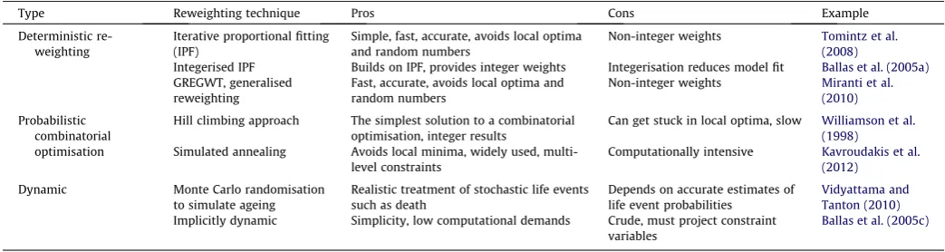
The wide range of methods available for spatial microsimula-tion can be divided into static, dynamic, deterministic and proba-bilistic approaches (Table 2). Static approaches generate small area microdata for one point in time. These can be classified as either probabilistic methods which use a random number genera-tor, and deterministic reweighting methods, which do not. The lat-ter produce fractional weights. Dynamic approaches project small area microdata into the future. They typically involve modelling of life events such as births, deaths and migration on the basis of random sampling from known probabilities on such events (Ballas et al., 2005a; Vidyattama & Tanton, 2010); more advanced agent-based techniques, such as spatial interaction models and house-hold-level phenomena, can be added to this basic framework (Wu et al., 2008; Wu, Birkin, & Rees, 2010). There are also ‘implic-itly dynamic’ models, which employ a static approach to reweight an existing microdata set to match projected change in aggregate-level variables (e.g.Ballas, Clarke, & Wiemers, 2005b).
2.2. IPF-based Monte Carlo approaches for the generation of synthetic microdata
Individual-level, anonymous samples from major surveys, such as the Sample of Anonymised Records (SARs) from the UK Census have only been available since around the turn of the century (Li, 2004). Beforehand, researchers had to rely on synthetic microdata. These can be created using probabilistic methods (Birkin & Clarke, 1988). The iterative proportional fitting (IPF) technique was first described in 1940 (Deming, 1940), and has become well estab-lished for spatial microsimulation (Birkin & Clarke, 1989; Axhau-sen, 2010).
The first application of IPF in spatial microsimulation was pre-sentedBirkin and Clarke (1988) and Birkin and Clarke (1989)to generate synthetic individuals, and allocate them to small areas based on aggregated data. They produced spatial microdata (a list of individuals and households for each electoral ward in Leeds Metropolitan District). Their approach was to select rows of syn-thetic data using Monte Carlo sampling. Birkin and Clarke sug-gested that the microdata generation technique known as ‘population synthesis’ could be of great practical use (Birkin & Clarke, 2012).
2.3. Combinatorial optimisation approaches
[image:3.595.31.285.87.182.2]Since the work ofBirkin and Clarke (1988) and Birkin and Clarke (1989)there have been considerable advances in data availability and computer hardware and software. In particular, with the emer-gence of anonymous survey data, the focus of spatial microsimula-tion shifted towards methods for reweighting and sampling from
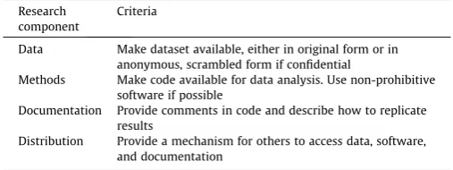
Table 1
Criteria for reproducible research, adapted fromPeng et al. (2006).
Research component
Criteria
Data Make dataset available, either in original form or in anonymous, scrambled form if confidential
Methods Make code available for data analysis. Use non-prohibitive software if possible
Documentation Provide comments in code and describe how to replicate results
Distribution Provide a mechanism for others to access data, software, and documentation
2
The code, data and instructions to replicate the findings are provided in the
existing microdata, as opposed to the creation of entirely synthetic data (Lee, 2009).
This has enabled experimentation with new techniques for small area microdata generation. A significant contribution to the literature was made byWilliamson et al. (1998). The authors pre-sented microsimulation as a problem ofcombinatorial optimisation: finding the combination of SARs which best fits the constraint vari-ables. Various approaches to combinatorial optimisation were compared, including ‘hill climbing’, simulated annealing ap-proaches and genetic algorithms (Williamson et al., 1998). These approaches involve the selection and replication of a discrete num-ber of individuals from a nationally representative list such as the SARs. Thus, subsets of individuals are taken from the global mic-rodataset (geocoded at coarse geographies) and allocated to small areas. There have been several refinements and applications of the original ideas suggested byWilliamson et al. (1998), including re-search reported by Voas and Williamson (2000), Williamson, Mitchell, and McDonald (2002), and Ballas, Clarke, and Dewhurst (2006).
2.4. Deterministic reweighting
The methods described in the previous section involve the use of random sampling procedures or ‘probabilistic reweighting’ ( Her-mes & Poulsen, 2012). In contrast, Ballas, Dorling, Thomas, and Rossiter (2005c)presented an alternative deterministic approach based on IPF. It is the results of this method, that does not use ran-dom number generators and thus produces the same output with each run,3that the integerisation methods presented here take as
their starting point. The underlying theory behind IPF has been de-scribed in a number of papers (Deming, 1940; Mosteller, 1968; Wong, 1992).Fienberg (1970)proves that IPF converges towards a single solution.
IPF can be used to produce maximum likelihood estimates of spatially disaggregated conditional probabilities for the individual attributes of interest. The method is also known as ‘matrix raking’, RAS or ‘entropy maximising’ (seeAxhausen, 2010; Birkin & Clarke, 1988; Huang & Williamson, 2001; Jiroušek & Prˇeucˇil, 1995; John-ston & Pattie, 1993; Kalantari, Lari, Ricca, & Simeone, 2008). The mathematical properties of IPF have been described in several pa-pers (see for instanceBirkin & Clarke, 1988; Bishop, Fienberg, & Holland, 1975; Fienberg, 1970). Illustrative examples of the proce-dure can be found in Saito (1992), Wong (1992) and Norman (1999). Wong (1992) investigated the reliability of IPF and evaluated the importance of different factors influencing its
performance; Simpson and Tranmer (2005) evaluated methods for improving the performance of IPF-based microsimulation. Building on these methods, IPF has been employed by others to investigate a wide range of phenomena (e.g.Ballas et al., 2005a; Mitchell, Shaw, & Dorling, 2000; Tomintz et al., 2008; Williamson et al., 2002).
Practical guidance on how to perform IPF for spatial microsim-ulation is also available. In an online working paper, Norman (1999)provides a user guide for a Microsoft Excel macro that per-forms IPF on large datasets.Simpson and Tranmer (2005)provided code snippets of their procedure in the statistical package SPSS.
Ballas et al. (2005c)describe the process and how it can be applied to problems of small area estimation. In addition to these re-sources, a practical guide to running IPF in R has been created to accompany this paper.4
2.5. Combinatorial optimisation, IPF and the need for integerisation
The aim of IPF, as with all spatial microsimulation methods, is to match individual-level data from one source to aggregated data from another. IPF does this repeatedly, using one constraint vari-able at a time: each brings the column and row totals of the simu-lated dataset closer to those of the area in question (see Ballas et al., 2005candFig. 5below).
Unlike combinatorial optimisation algorithms, IPF results in non-integer weights. As mentioned above, this is problematic for certain applications. In their overview of methods for spatial microsimulationWilliamson et al. (1998)favoured combinatorial optimisation approaches, precisely for this reason: ‘‘as non-integer weights lead, upon tabulation of results, to fractions of households or individuals’’ (p. 791). There are two options available for dealing with this problem with IPF:
Use combinatorial optimisation microsimulation methods instead (Williamson et al., 1998). However, this can be compu-tationally intensive (Pritchard & Miller, 2012).
Integerise the weights: Translate the non-integer weights obtained through IPF into discrete counts of individuals selected from the original survey dataset (Ballas et al., 2005a).
We revisit the second option, which arguably provides the ‘best of both worlds’: the simplicity and computational speed of deter-ministic reweighting and the benefits of using whole cases.
[image:4.595.41.563.86.225.2]In summary, IPF is an established method for combining microdata with spatially aggregated constraints to simulate target
Table 2
Typology of spatial microsimulation methods.
Type Reweighting technique Pros Cons Example
Deterministic re-weighting
Iterative proportional fitting (IPF)
Simple, fast, accurate, avoids local optima and random numbers
Non-integer weights Tomintz et al. (2008)
Integerised IPF Builds on IPF, provides integer weights Integerisation reduces model fit Ballas et al. (2005a)
GREGWT, generalised reweighting
Fast, accurate, avoids local optima and random numbers
Non-integer weights Miranti et al. (2010)
Probabilistic combinatorial optimisation
Hill climbing approach The simplest solution to a combinatorial optimisation, integer results
Can get stuck in local optima, slow Williamson et al. (1998)
Simulated annealing Avoids local minima, widely used, multi-level constraints
Computationally intensive Kavroudakis et al. (2012)
Dynamic Monte Carlo randomisation to simulate ageing
Realistic treatment of stochastic life events such as death
Depends on accurate estimates of life event probabilities
Vidyattama and Tanton (2010)
Implicitly dynamic Simplicity, low computational demands Crude, must project constraint variables
Ballas et al. (2005c)
3
Probabilistic results can also be replicated, by ‘setting the seed’ of a predefined set of pseudo-random numbers.
4
variables whose characteristics are not recorded at the local level. Intergerisation translates the real number weights obtained by IPF into samples from the original microdata, a list of ‘cloned’ individ-uals for each simulated area. Integerisation may also be useful con-ceptually, as it allows researchers to deal with entire individuals. The next section reviews existing strategies for integerisation.
3. Method
Despite the importance of integer weights for dynamic spatial microsimulation, and the continued use of IPF, there has been little work directed towards integerisation. It has been noted that ‘‘the integerization and the selection tasks may introduce a bias in the synthesized population’’ (Axhausen, 2010, p. 10), yet little work has been done to find outhow mucherror is introduced.
To test each integerisation method, IPF was used to generate an array of weights that fit individual-level survey data to geograph-ically aggregated Census data (see Section3.7). Five methods for integerising the results are described, three deterministic and two probabilistic. These are: ‘simple rounding’, its evolution into the ‘threshold approach’ and the ‘counter-weight’ method and the probabilistic methods ‘proportional probabilities’ and finally ‘truncate, replicate, sample’. TRS builds on the strengths of the other methods, hence the order in which they are presented.
The application of these methods to the same dataset (and their implementation in the same language, R) allows their respective performance characteristics to be quantified and compared. Before proceeding to describe the mechanisms by which these integerisa-tion methods work, it is worth taking a step back, to consider the nature and meaning of IPF weights.
3.1. Interpreting IPF weights: replication and probability
It is important to clarify what we mean by ‘weights’ before pro-ceeding to implement methods of integerisation: this understand-ing was central to the development of the integerisation method presented in this paper. The weights obtained through IPF are real numbers ranging from 0 to hundreds (the largest weight in the case study dataset is 311.8). This range makes integerisation prob-lematic: if the probability of selection is proportional to the IPF weights (as is the case with the ‘proportional probabilities’ meth-od), the majority of resulting selection probabilities can be very low. This is why the simple rounding method rounds weights up or down to the nearest integer weight to determine how many times each individual should be replicated (Ballas et al., 2005a): to ensure replication weights do not differ greatly from non-inte-ger IPF weights. However, some of the information contained in the weight is lost during rounding: a weight remainder of 0.501 is treated the same as 0.999.
This raises the following question: Do the weights refer to the number of times a particular individual should be replicated, or is it related to the probability of being selected? The following sec-tions consider different approaches to addressing this question, and the integerisation methods that result.
3.2. Simple rounding
The simplest approach to integerisation is to convert the non-integer weights into an non-integer by rounding. If the decimal remain-der to the right of the decimal is 0.5 or above, the integer is rounded up; if not, the integer is rounded down.
Rounding alone is inadequate for accurate results, however. As illustrated inFig. 2below, the distribution of weights obtained by IPF is likely to be skewed, and the majority of weights may fall be-low the critical 0.5 value and be excluded. As reported byBallas
et al. (2005a, p. 25), this results in inaccurate total populations. To overcome this problemBallas et al. (2005a) developed algo-rithms to ‘top up’ the simulated spatial microdata with representa-tive individuals: the ‘threshold’ and ‘counter-weight’ approaches.
3.3. The threshold approach
Ballas et al. (2005a)tackled the need to ‘top up’ the simulated area populations such thatPopsimPPopcens. To do this, an inclusion
threshold (IT) is created, set to 1 and then iteratively reduced (by 0.001 each time), adding extra individuals with incrementally low-er weights.5Below the exit value ofITfor each zone, no individuals can be included (hence the clear cut-off point around 0.4 inFig. 1). In its original form, based on rounded weights, this approach over-rep-licates individuals with high decimal weights. To overcome this problem, we took the truncated weights as the starting population, rather than the rounded weights. This modified approach improved the accuracy of the integer results and is therefore what we refer to when the ‘threshold approach’ is mentioned henceforth.6
The technique successfully tops-up integer populations yet has a tendency to generate too many individuals for each zone. This oversampling is due to duplicate weights – each unique weight was repeated on average three times in our model – and the pres-ence of weights thataredifferent, but separated by less than 0.001. (In our test, the mean number of unique weights falling into non-empty bins between 0.3 and 0.48 in each area – the range of values reached byITbeforePopsimPPopcens– is almost two.).
3.4. The counter-weight approach
An alternative method for topping-up integer results arrived at by simple rounding was also described byBallas et al. (2005a). The approach was labelled to emphasise its reliance on both counter and a weight variables. Each individual is first allocated a counter in ascending order of its IPF weight. The algorithm then tops-up the integer results of simple rounding by iterating over all individ-uals in the order of their count. With each iteration the new integer weight is set as the rounded weight plus the rounded sum of its decimal weight plus the decimal weight of the next individual, un-til the desired total population is reached.7
There are two theoretical advantages of this approach: its more accurate final populations (it does not automatically duplicate individuals with equal weights as the threshold approach does) and the fact that individuals with decimal weights down to 0.25 may be selected. This latter advantage is minor, asITreached be-low 0.4 in many cases (Supplementary information, Fig. 2) – not far off. A band of low weights (just above 0.25) selected by the counter-weight method can be seen inFig. 1.
The total omission of weights below some threshold is prob-lematic for all deterministic algorithms tested here: they imply that someone with a weight below this threshold, for Example 0.199 in our tests, has the same sampling probability as someone with a weight of 0.001: zero! The complete omission of low weights fails to make use of all the information stored in IPF
5
A more detailed description of the steps taken and the R code needed to perform them iteratively can be found in theSupplementary Information, Section3.2.
6
An explanation of this improvement can be illustrated by considering an individual with a weight of 2.99. Under the original threshold approach described byBallas et al. (2005a), this person would be replicated four times: three times after rounding, and then a fourth time afterITdrops below 0.99. With our modified approach they would be replicated three times: twice after truncation, and again after
ITdrops below 0.99. The improvement in accuracy in our tests was substantial, from a TAE (total absolute error, described below) of 96,670–66,762. Because both methods are equally easy to implement, we henceforth refer only to the superior version of the threshold integerisation method.
7
weights: in fact, the individual with an IPF weight of 0.199 is 199 times more representative of the area (in terms of the constraint variables and the make-up of the survey dataset) than the individ-ual with an IPF weight of 0.001. Probabilistic approaches to intege-risation ensure that all such differences between decimal weights are accounted for.
3.5. The proportional probabilities approach
This approach to integerisation treats IPF weights as probabili-ties. The chance of an individual being selected is proportional to the IPF weight:
p¼PwW ð1Þ
Sampling untilPopsim=Popcenswith replicationensures that
individ-uals with high weights are likely to be repeated several times whereas individuals with low weights are unlikely to appear. The outcome of this strategy is correct from a theoretical perspective, yet because all weights are treated as probabilities, there is a non-zero chance that an individual with a low weight (e.g. 0.3) is repli-cated more times than an individual with a higher weight (e.g. 3.3). (In this case the probability for any given area is1%, regardless of the population size). Ideally, this should never happen: the individ-ual with weight 0.3 should be replicated either 0 or 1 times, the probability of the latter being 0.3. The approach described in the next section addresses these issues.
3.6. Truncate, replicate, sample
The problems associated with the aforementioned integerisa-tion strategies demonstrate the need for an alternative method. Ideally, the method would build upon the simplicity of the round-ing method, select the correct simulated population size (as at-tempted by the threshold approach and achieved by using ‘proportional probabilities’), make use of all the information stored in IPF weightsandreduce the error introduced by integerisation to a minimum. The probabilistic approach used in ‘proportional prob-abilities’ allows multiple answers to be calculated (by using differ-ent ‘seeds’). This is advantageous for analysis of uncertainty introduced by the process and allows for the selection of the best fitting result. Consideration of these design criteria led us to devel-op TRS integerisation, which interprets weights as follows: IPF
weights do not merely represent the probability of a single case being selected. They also (when above one) contain information about repetition: the two types of weight are bound up in a single number. An IPF weight of 9, for example, means that the individual should be replicated nine times in the synthetic microdataset. A weight of 0.2, by contrast, means that the characteristics of this individual should count for only 1/5 of their whole value in the microsimulated dataset and that, in a representative sampling strategy, the individual would have a probability of 0.2 of being se-lected. Clearly, these are different concepts. As such, the TRS ap-proach to integerisation isolates the replication and probability components of IPF weights at the outset, and then deals with each separately. Simple rounding, by contrast, interprets IPF weights as inaccurate count data. The steps followed by the TRS approach are described in detail below.
3.6.1. Truncate
By removing all information to the right of the decimal point, truncation results in integer values – integer replication weights that determine how many times each individual should be ‘cloned’ and placed into the simulated microdataset. In R, the following command is used:
count<truncðwÞ
wherewis a matrix of individual weights. Saving these values (as
count) will later ensure that only whole integers are counted. The decimal remainders (dr), which vary between 0 and 1, are saved by subtracting the integer weights from the full weights:
dr<wcount
This separation of conventional and replication weights provides the basis for the next stage: replication of the integer weights.
3.6.2. Replicate
In spreadsheets, replication refers simply to copying cells of data and pasting them elsewhere. In spatial microsimulation, the concept is no different. The number of times a row of data is rep-licated depends on the integer weight: an IPF weight of 0.99, for example, would not be replicated at this stage because the integer weight (obtained through truncation) is 0.
[image:6.595.91.519.66.258.2]To reduce the computational requirements of this stage, it is best to simply replicate the row number (index) associated with each individual, rather than replicate the entire row of data. This
is illustrated in the following code example, which appears within a loop for each area (i) to be simulated:
ints½½i<index½repð1:nrowðindexÞ;countÞ
Here, the indices (of weights above 1,index) are selected and
then repeated. This is done using the functionrep (). The first argument (1:nrow (index)) simply defines the indices to be rep-licated; the second (count) refers to the integer weights defined in the previous subsection. (Note:countin this context refers only to the integer weights above 1 in each area). Once the replicated indi-ces have been generated, they can then be used to look up the rel-evant characteristics of the individuals in question.
3.6.3. Sample
As with the rounding approach, the truncation and replication stages alone are unable to produce microsimulated datasets of the correct size. The problem is exacerbated by the use of trunca-tion instead of rounding: truncatrunca-tion is guaranteed to produce inte-ger microdataset populations that are smaller, and in some cases much smaller than the actual (census) populations. In our case study, the simulated microdataset populations were around half the actual size populations defined by the census. This under-selection of whole cases has the following advantage: when using truncation there is no chance of over-sampling, avoiding the prob-lem of simulated populations being slightly too large, as can occur with the threshold approach.
Given that the replication weights have already been included in steps 1 and 2, only the decimal weight remainders need to be in-cluded. This can be done using weighted random sampling without replacement. In R, the following function is used:
sampleðw;size¼ ðpops½i;1 pops½i;2Þ;prob ¼ dr½;iÞ
Here, the argumentsizewithin thesamplecommand is set as the difference between the known population of each area (pops[i,1]) and the size obtained through the replication stage alone ( pop-s[i,2]). The probability (prob) of an individual being sampled is determined by the decimal remainders. drvaries between 0 and 1, as described above.
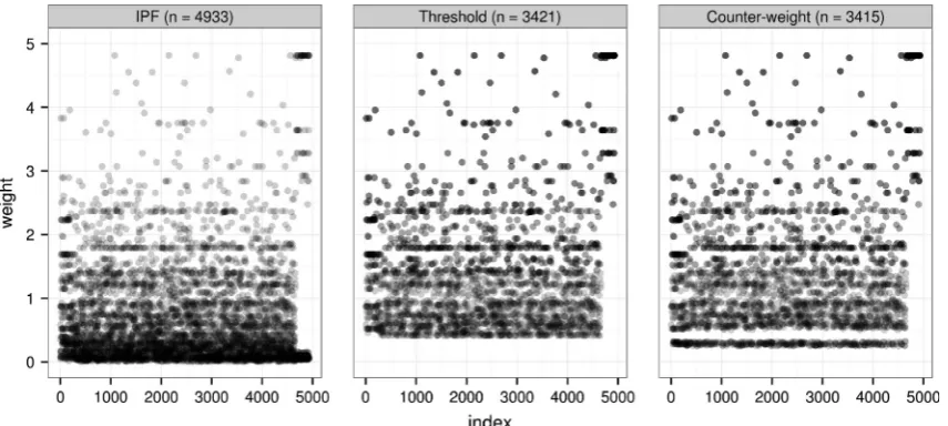
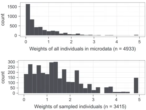
The results for one particular area are presented inFig. 2. The distribution of selected individuals has shifted to the right, as the replication stage has replicated individuals as a function of their truncated weight. Individuals with low weights (below one) still constitute a large portion of those selected, yet these individuals are replicated fewer times. After TRS integerisation individuals with high decimal weights are relatively common. Before
integerisation, individuals with IPF weights between 0 and 0.3 dominated. An individual-by-individual visualisation of the Monte Carlo sampling strategy is provided inFig. 3. Comparing this with the same plot for the probabilistic methods (Fig. 1), the most noticeable difference is that the TRS and proportional probabilities approaches include individuals with very low weights. Another important difference is average point density, as illustrated by the transparency of the dots: inFig. 1, there are shifts near the dec-imal weight threshold (0.4 in this area) on they-axis. InFig. 3, by contrast, the transition is smoother: average darkness of single dots (the number of replications) gradually increases from 0 to 5 in both probabilistic methods.
Fig. 4 illustrates the mechanism by which the TRS sampling strategy works to select individuals. In the first stage (up to
x= 1717, in this case) there is a linear relationship between the indices of survey and sampled individuals, as the model iteratively moves through the individuals, replicating those with truncated weights greater than 0. This (deterministic) replication stage se-lects roughly half of the required population in our example data-set (this proportion varies from zone to zone). The next stage is probabilistic sampling (x= 1718 onwards in Fig. 4): individuals are selected from the entire microdataset with selection probabil-ities equal to weight remainders.
3.7. The test scenario: input data and IPF
The theory and methods presented above demonstrate how five integerisation methods work in abstract terms. But to compare them quantitatively a test scenario is needed. This example con-sists of a spatial microsimulation model that uses IPF to model the commuting and socio-demographic characteristics of econom-ically active individuals in Sheffield. According to the 2001 Census, Sheffield has a working population of just over 230,000. The char-acteristics of these individuals were simulated by reweighting a synthetic microdataset based on aggregate constraint variables provided at the medium super output area (MSOA) level. The syn-thetic microdataset was created by ‘scrambling’ a subset of the Understanding Society dataset (USd).8 MSOAs contain on average just over 7000 people each, of whom 44% are economically active in the study area; for the less sensitive aggregate constraints, real data were used. These variables are summarised inTable 3.
The data contains both continuous (age, distance) and categor-ical (mode, NS-SEC) variables. In practice, all variables are con-verted into categorical variables for the purposes of IPF, however. To do this statistical bins are used.Table 3illustrates similarities between aggregate and survey data overall (car drivers being the most popular mode of travel to work in both categories, for exam-ple). Large differences exist between individual zones and survey data, however: it is the role of iterative proportional fitting to apply weights to minimise these differences.
IPF was used to assign 71 weights to each of the 4933 individ-uals, one weight for each zone. The fit between census and weighted microdata can be seen improving after constraining by each of the 40 variables (Fig. 5). The process is repeated until an adequate level of convergence is attained (seeFig. 6).9The weights
were set to an initial value of one.10The weights were then itera-0
500 1000 1500
0 1 2 3 4 5
Weights of all individuals in microdata (n = 4933)
count
0 50 100 150 200 250 300
0 1 2 3 4 5
Weights of sampled individuals (n = 3415)
[image:7.595.41.277.64.241.2]count
Fig. 2.Histograms of original microdata weights (above) and sampled microdata after TRS integerisation (below) for a single area — zone 71 in the case study data.
8Seehttp://www.understandingsociety.org.uk/. To scramble this data, the
contin-uous variables (seeTable 3) had an integer random number (between 10 and10) added to them; categorical variables were mixed up, and all other information was removed.
9What constitutes an ‘adequate’ level of fit has not been well defined in the
literature, as mentioned in the next section. In this example, 20 iterations were used.
10
tively altered to match the aggregate (MSOA) level statistics, as de-scribed in Section2.4.
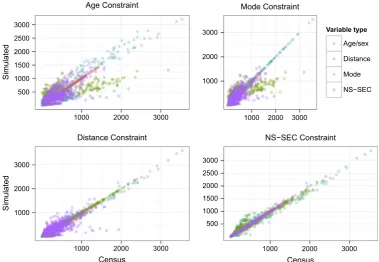
Four constraint variables link the aggregated census data to the survey, containing a total of 40 categories. To illustrate how IPF works, it is useful to inspect the fit between simulated and census aggregates before and after performing IPF for each constraint var-iable.Fig. 5illustrates this process for each constraint. By contrast to existing approaches to visualising IPF (seeBallas et al., 2005c),
Fig. 5plots the results for all variables, one constraint at a time. This approach can highlight which constraint variables are partic-ularly problematic. After 20 iterations (Fig. 6), one can see that dis-tance and mode constraints are most problematic. This may be because both variables depend largely on geographical location, so are not captured well by UK-wide aggregates.
Fig. 5also illustrates how IPF works: after reweighting for a par-ticular constraint, the weights are forced to take values such that the aggregate statistics of the simulated microdataset match per-fectly with the census aggregates, for all variables within the con-straint in question. Aggregate values for the mode variables, for example, fit the census results perfectly after constraining by mode (top right panel inFig. 5). Reweighting by the next constraint dis-rupts the fit imposed by the previous constraint – note the increase scatter of the (blue) mode variables after weights are constrained by distance (bottom left).
However, the disrupted fit is better than the original. This leads to a convergence of the weights such that the fit between simu-lated and known variables is optimised:Fig. 5shows that accuracy increases after weights are constrained by each successive linking variable.
4. Results
This section compares the five previously describe approaches to integerisation – rounding, inclusion threshold, counter-weight, proportional probabilities and TRS methods. The results are based on the 20th iteration of the IPF model described above. The follow-ing metrics of performance were assessed:
Speed of calculation.
Accuracy of results. – Sample size.
– Total Absolute Error (TAE) of simulated areas.
– Anomalies (aggregate cell values out by more than 5%). – Correlation between constraint variables in the census and
microsimulated data.
Of these performance indicators accuracy is the most problem-atic. Options for measuring goodness-of-fit have proliferated in the last two decades, yet there is no consensus about which is most appropriate (Voas & Williamson, 2001). The approach taken here, therefore, is to use a range of measures, the most important of which are summarised inTable 4andFig. 7.
4.1. Speed of calculation
[image:8.595.91.520.66.259.2]The time taken for the integerisation of IPF weights was mea-sured on an Intel Core i5 660 (3.33 GHz) machine with 4 Gb of
Fig. 3.Overplotted scatter graphs of index against weight for the original IPF weights (left) and after proportional probabilities (middle) and TRS (right) integerisation for zone 71. Compare withFig. 1.
1000 2000 3000 4000
500 1000 1500 2000 2500
Index of simulated area
Survey index
[image:8.595.50.287.305.461.2]Fig. 4.Scatter graph of the index values of individuals in the original sample and their indices following TRS Integerisation for a single area.
Table 3
Summary data for the spatial microsimulation model.
Aggregate data Survey data 71 Zones, average pop.: 3077.5 4933 observations Variable N. categories Most populous Mean Most populous Age/sex 12 Male, 35–54 yrs 40.1 –
Mode 11 Car driver – Car driver
Distance 8 2–5 km 11.6 –
[image:8.595.41.290.679.755.2]RAM running Linux 3.0. The simple rounding method of integerisa-tion was unsurprisingly the fastest, at 4 s. In second and third place respectively were the proportional probabilities and TRS ap-proaches, which took a couple of seconds longer for a single intege-risation run for all areas. Slowest were the inclusion threshold and counter-weight techniques, which took three times longer than simple rounding. To ensure representative results for the probabilis-tic approaches, both were run 20 times and the result with the best fit was selected. These imputation loops took just under a minute.
The computational intensity of integerisation may be problem-atic when processing weights for very large datasets, or using older computers. However, the results must be placed in the context of the computational requirements of the IPF process itself. For the example described in Section 3.7, IPF took approximately 30 s per iteration and 5 min for the full 20 iterations.
4.2. Accuracy
In order to compare the fit between simulated microdata and the zonally aggregated linking variables that constrain them, the
former must first be aggregated by zone. This aggregation stage al-lows the fit between linking variables to be compared directly (see
Fig. 7). More formally, this aggregation allows goodness of fit to be calculated using a range of metrics (Williamson et al., 1998). We compared the accuracy of integerisation techniques using five metrics:
Pearson’s product-moment correlation coefficient (r).
Total and standardised absolute error (TAE and SAE).
Proportion of simulated values falling beyond 5% of the actual values.
The proportion ofZ-scores significant at the 5% level.
Size of the sampled populations,
The simplest way to evaluate the fit between simulated and census results was to use Pearson’sr, an established measure of association (Rodgers, 1988). Thervalues for all constraints were 0.9911, 0.9960, 0.9978, 0.9989 and 0.9992 for rounding, thresh-old, counter-weight, proportional probabilities and TRS methods respectively. IPF alone had anrvalue of 0.9996. These correlations establish an order of fit that can be compared to other metrics.
TAE and SAE are crude yet effective measures of overall model fit (Voas & Williamson, 2001). TAE has the additional advantage of being easily understood:
TAE¼X ij
jUijTijj ð2Þ
whereUandTare the observed and simulated values for each link-ing variable (j) and each area (i). SAE is the TAE divided by the total population of the study area. TAE is sensitive to the number of peo-ple within the model, while SAE is not. The latter is seen byVoas and Williamson (2001)as ‘‘marginally preferable’’ to the former: it allows cross-comparisons between models of different total pop-ulations (Kongmuang, 2006).
500 1000 1500 2000 2500 3000
1000 2000 3000
Age Constraint
Simulated 1000
2000 3000
1000 2000 3000
Mode Constraint
Variable type
Age/sex
Distance
Mode
NS−SEC
1000 2000 3000
1000 2000 3000
Distance Constraint
Census
Simulated
500 1000 1500 2000 2500 3000
1000 2000 3000
NS−SEC Constraint
[image:9.595.102.482.67.329.2]Census
Fig. 5.Visualisation of IPF method. The graphs show the iterative improvements in fit after age, mode, distance and finally NS-SEC constraints were applied (seeTable 3). See Footnote 4 for resources on how IPF works.
500 1000 1500 2000 2500 3000
1000 2000 3000
Census
Simulated Constraint
Age/sex Distance Mode NS−SEC
[image:9.595.48.270.382.508.2]The proportion of values which fall beyond 5% of the actual val-ues is a simple metric of the quality of the fit. It implies that getting a perfect fit is not the aim, and penalises fits that have a large num-ber of outliers. The precise definition of ’outlier’ is somewhat arbi-trary (one could just as well use 1%).
The final metric presented inTable 4is based on theZ-statistic, a standardised measure of deviance from expected values, calcu-lated for each cell of data. We useZm, a modified version of the
Z-statistic which is a robust measure of fit for each cell value Wil-liamson et al. (1998). The measure of fit is appropriate here as it
takes into account absolute, rather than just relative, differences between simulated and observed cell count:
Zmij¼ ðrijpijÞ
pijð1pijÞ
P ijUij
!1=2 ,
ð3Þ
where
pij¼
Uij
P ijUij
and rij¼
Tij
[image:10.595.129.478.86.380.2]P ijUij
Table 4
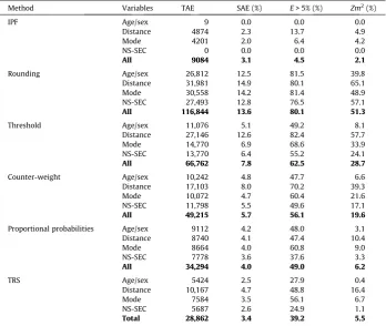
Accuracy results for integerisation techniques.a
Method Variables TAE SAE (%) E> 5% (%) Zm2
(%)
IPF Age/sex 9 0.0 0.0 0.0
Distance 4874 2.3 13.7 4.9
Mode 4201 2.0 6.4 4.2
NS-SEC 0 0.0 0.0 0.0
All 9084 3.1 4.5 2.1
Rounding Age/sex 26,812 12.5 81.5 39.8
Distance 31,981 14.9 80.1 65.1
Mode 30,558 14.2 81.4 48.9
NS-SEC 27,493 12.8 76.5 57.1
All 116,844 13.6 80.1 51.3
Threshold Age/sex 11,076 5.1 49.2 8.1
Distance 27,146 12.6 82.4 57.7
Mode 14,770 6.9 68.6 33.9
NS-SEC 13,770 6.4 55.2 24.1
All 66,762 7.8 62.5 28.7
Counter-weight Age/sex 10,242 4.8 47.7 6.6
Distance 17,103 8.0 70.2 39.3
Mode 10,072 4.7 60.4 21.6
NS-SEC 11,798 5.5 49.6 17.1
All 49,215 5.7 56.1 19.6
Proportional probabilities Age/sex 9112 4.2 48.0 3.1
Distance 8740 4.1 47.4 10.4
Mode 8664 4.0 60.8 9.0
NS-SEC 7778 3.6 37.6 3.3
All 34,294 4.0 49.0 6.2
TRS Age/sex 5424 2.5 27.9 0.4
Distance 10,167 4.7 48.8 16.4
Mode 7584 3.5 56.1 6.7
NS-SEC 5687 2.6 24.9 1.1
Total 28,862 3.4 39.2 5.5
aThe probabilistic results represent the best fit (in terms of TAE) of 20 integerisation runs with the
pseudo-random number seed set to 1000 for replicability – seeSupplementary information.
Rounding Threshold Counter−weight Prop−prob TRS
0 1000 2000 3000
0 2000 0 2000 0 2000 0 2000 0 2000
Census
Simulated
Constraint
Age/sex
Distance
Mode
NS−SEC
[image:10.595.111.493.420.610.2]To use the modifiedZ-statistic as a measure of overall model fit, one simply sums the squares ofzmto calculateZm2. This measure
can handle observed cell counts below 5, which chi-squared tests cannot (Voas & Williamson, 2001).
The results presented inTable 4confirm thatallintegerisation methods introduce some error. It is reassuring that the compara-tive accuracy is the same across all metrics. Total absolute error (TAE), the simplest goodness-of-fit metric, indicates that discrep-ancies between simulated and census data increase by a factor of 3.2 after TRS integerisation, compared with raw (fractional) IPF weights.11Still, this is a major improvement on the simple rounding,
threshold and counter-weight approaches to integerisation pre-sented byBallas et al. (2005a): these increased TAE by a factor of 13, 7 and 5 respectively. The improvement in fit relative to the pro-portional probabilities method is more modest. The propro-portional probabilities method increased TAE by a factor of 3.8, 23% more absolute error than TRS.
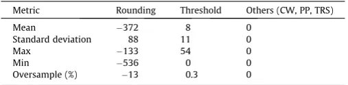
The differences between the simulated and actual populations (PopsimPopcens) were also calculated for each area. The resulting
differences are summarised inTable 5, which illustrates that the counter-weight and two probabilistic methods resulted in the cor-rect population totals for every area. Simple rounding and thresh-old integerisation methods greatly underestimate and slightly overestimate the actual populations, respectively.
5. Discussion and conclusions
The results show that TRS integerisation outperforms the other methods of integerisation tested in this paper. At the aggregate le-vel, accuracy improves in the following order: simple rounding, inclusion threshold, counter-weight, proportional probabilities and, most accurately, TRS. This order of preference remains un-changed, regardless of which (from a selection of 5) measure of goodness-of-fit is used. These results concur with a finding derived from theory – that ‘‘deterministic rounding of the counts is not a satisfactory integerization’’ (Pritchard & Miller, 2012, p. 689). Pro-portional probability and TRS methods clearly provide more accu-rate alternatives.
An additional advantage of the probabilistic TRS and propor-tional probability methods is that correct population sizes are guaranteed.12 In terms of speed of calculation, TRS also performs
well. TRS takes marginally more time than simple rounding and pro-portional probability methods, but is three times quicker than the threshold and counter-weight approaches. In practice, it seems that integerisation processing time is small relative to running IPF over several iterations. Another major benefit of these non-deterministic methods is that probability distributions of results can be generated,
if the algorithms are run multiple times using unrelated pseudo-ran-dom numbers. Probabilistic methods could therefore enable the uncertainty introduced through integerisation to be investigated quantitatively (Beckman et al., 1996; Little & Rubin, 1987) and sub-sequently illustrated using error bars.
Overall the results indicate that TRS is superior to the determin-istic methods on many levels and introduces less error than the proportional probabilities approach. We cannot claim that TRS is ‘the best’ integerisation strategy available though: there may be other solutions to the problem and different sets of test weights may generate different results.13The issue will still present a
chal-lenge for future researchers considering the use of IPF to generate sample populations composed of whole individuals: whether to use deterministic or probabilistic methods is still an open question (some may favour deterministic methods that avoid psuedo-random numbers, to ensure reproducibility regardless of the software used), and the question of whether combinatorial optimisation algorithms perform better has not been addressed.
Our results provide insight into the advantages and disadvan-tages of five integerisation methods and guidance to researchers wishing to use IPF to generate integer weights: use TRS unless determinism is needed or until superior alternatives (e.g. real small area microdata) become available. Based on the code and example datasets provided in the Supplementary Information, we encourage others to use, build-on and improve TRS integerisation.
A broader issue raised by the this research, that requires further investigation before answers emerge, is ‘how do the integerised re-sults of IPF compare with combinatorial optimisation approaches to spatial microsimulation?’ Studies have compared non-integer results of IPF with alternative approaches (Harland et al., 2012; Rahman, Harding, & Tanton, 2010; Ryan, Maoh, & Kanaroglou, 2009; Smith, Clarke, & Harland, 2009). However, these have so far failed to compare like with like: the integer results of combina-torial approaches are more useful (applicable to more types of analysis) than the non-integer results of IPF. TRS thus offers a way of ‘levelling the playing field’ whilst minimising the error introduced to the results of deterministic re-weighting through integerisation.
In conclusion, the integerisation methods presented in this pa-per make integer results accessible to those with a working knowledge of IPF. TRS outperforms previously published methods of integerisation. As such, the technique offers an attractive alter-native to combinatorial optimisation approaches for applications that require whole individuals to be simulated based on aggre-gate data.
Acknowledgements
[image:11.595.32.286.86.148.2]Thanks to: Milan Delor, Mark Green, Luke Temple, David Ander-son and Krystyna Koziol for proof reading and suggestions; to Eve-line van Leeuwen for testing the methods on real data and improving the code; and to the anonymous reviewers for construc-tive comments. This research was funded by the Engineering and Physical Sciences Research council (EPSRC) the via the E-Futures Doctoral Training Centre.
Table 5
Differences between census and simulated populations.
Metric Rounding Threshold Others (CW, PP, TRS)
Mean 372 8 0
Standard deviation 88 11 0
Max 133 54 0
Min 536 0 0
Oversample (%) 13 0.3 0
11
In the case of a sufficiently diverse input survey dataset, IPF would be able to find the perfect solution: TAE would be 0 and the ratio of error would not be applicable.
12
Although the counter-weight method produced the correct population sizes in our tests, it cannot be guaranteed to do so in all cases, because of its reliance on simple rounding: if more weights are rounded up than down, the population will be too high. However, it can be expected to yield the correct population in cases where the populations of the areas under investigation are substantially larger than the number of individuals in the survey dataset.
13
Appendix A. Supplementary data
Supplementary data associated with this article can be found, in the online version, athttp://dx.doi.org/10.1016/j.compenvurbsys. 2013.03.004.
References
Anderson, B. (2007). Creating small area income estimates for England: spatial microsimulation modelling. Technical Report. University of Essex.
Anderson, B. (2013). Estimating small-area income deprivation: an iterative proportional fitting approach. In R. Tanton, K. Edwards (Eds.), Spatial microsimulation: a reference guide for users. Understanding population trends and processes(Vol. 6, pp. 49–67). Netherlands: Springer (Chapter 4). Axhausen, K., & Müller, K. (2010).Population synthesis for microsimulation: State of
the art. Technical Report August. Swiss Federal Institute of Technology Zurich.
Ballas, D., Clarke, G. P., & Dewhurst, J. (2006). Modelling the socio-economic impacts of major job loss or gain at the local level: A spatial microsimulation framework.
Spatial Economic Analysis, 1, 127–146.
Ballas, D., Clarke, G., Dorling, D., Eyre, H., Thomas, B., & Rossiter, D. (2005a). SimBritain: A spatial microsimulation approach to population dynamics.
Population, Space and Place, 11, 13–34.
Ballas, D., Clarke, G. P., & Wiemers, E. (2005b). Building a dynamic spatial microsimulation model for Ireland.Population, Space and Place, 11, 157–172.
Ballas, D., Dorling, D., Thomas, B., & Rossiter, D. (2005c). Geography matters: Simulating the local impacts of national social policies. York, UK: Joseph Roundtree Foundation.
Ballas, D., O’Donoghue, C., Clarke, G., Hynes, S., & Morrissey, K. (2013).A review of microsimulation for policy analysis. Springer. Chapter 3, p. 264.
Beckman, R., Baggerly, K., & McKay, M. (1996). Creating synthetic baseline populations.Transportation Research Part A: Policy and Practice, 30, 415–429. Birkin, M., & Clarke, M. (2011). Spatial microsimulation models: A review and a
glimpse into the future. In J. Stillwell, M. Clarke, J. Stillwell (Eds.),Population dynamics and projection methods. Understanding population trends and processes
(Vol. 4, pp. 193–208). Netherlands: Springer.
Birkin, M., & Clarke, M. (1988). SYNTHESIS – A synthetic spatial information system for urban and regional analysis: Methods and examples. Environment and Planning A, 20, 1645–1671.
Birkin, M., & Clarke, M. (1989). The generation of individual and household incomes at the small area level using synthesis.Regional Studies, 23, 535–548.
Birkin, M., & Clarke, G. (2012). The enhancement of spatial microsimulation models using geodemographics.The Annals of Regional Science, 49, 515–532.
Bishop, Y., Fienberg, S., & Holland, P. (1975).Discrete multivariate analysis: theory and practice. Cambridge, Massachusettes: MIT Press.
Clarke, M. (1986). Demographic processes and household dynamics: A microsimulation approach. In: R. Woods, P.H. Rees (Eds.),Population structures and models: Developments in spatial demography(pp. 245–272).
Deming, W. (1940). On a least squares adjustment of a sampled frequency table when the expected marginal totals are known.The Annals of Mathematical Statistics.
Edwards, K. L., & Clarke, G. P. (2009). The design and validation of a spatial microsimulation model of obesogenic environments for children in Leeds, UK: SimObesity.Social Science & Medicine, 69, 1127–1134.
Fienberg, S. (1970). An iterative procedure for estimation in contingency tables.The Annals of Mathematical Statistics, 41, 907–917.
Gentleman, R., & Temple Lang, D. (2007). Statistical analyses and reproducible research.Journal of Computational and Graphical Statistics, 16, 1–23.
Gilbert, G. N. (2008).Agent-based models. New York: Sage Publications.
Gilbert, N., & Troitzsch, K. G. (2005).Simulation for the social scientist. New York: McGraw-Hill International.
Goffe, W. L., Ferrier, G. D., & Rogers, J. (1994). Global optimization of statistical functions with simulated annealing.Journal of Econometrics, 60, 65–99.
Harland, K., Heppenstall, A., Smith, D., & Birkin, M. (2012). Creating realistic synthetic populations at varying spatial scales: A comparative critique of population synthesis techniques. Journal of Artificial Societies and Social Simulation, 15, 1.
Hermes, K., & Poulsen, M. (2012). A review of current methods to generate synthetic spatial microdata using reweighting and future directions. Computers, Environment and Urban Systems, 36, 281–290.
Holm, E., Lindgren, U., Malmberg, G., & Mäkilä, K. (1996). Simulating an entire nation. In: G.P. Clarke (Ed.), Microsimulation for urban and regional policy analysis.European research in regional science(Pion. 6, pp. 164–186). Hooimeijer, P. (1996). A life-course approach to urban dynamics: State of the art in
and research design for the Netherlands. In G.P. Clarke (Ed.),Microsimulation for urban and regional policy analysis(pp. 28–63). Pion, London.
Huang, Z., & Williamson, P. (2001).The creation of a national set of validated small area population microdata. Technical Report October. University of Liverpool.
Hynes, S., Morrissey, K., ODonoghue, C., & Clarke, G. (2009). A spatial micro-simulation analysis of methane emissions from Irish agriculture.Ecological Complexity, 6, 135–146.
Ince, D. C., Hatton, L., & Graham-Cumming, J. (2012). The case for open computer programs.Nature, 482, 485–488.
Jiroušek, R., & Prˇeucˇil, S. (1995). On the effective implementation of the iterative proportional fitting procedure. Computational Statistics & Data Analysis, 19, 177–189.
Johnston, R. J., & Pattie, C. J. (1993). Entropy-maximizing and the iterative proportional fitting procedure.The Professional Geographer, 45, 317–322.
Kalantari, B., Lari, I., Ricca, F., & Simeone, B. (2008). On the complexity of general matrix scaling and entropy minimization via the RAS algorithm.Mathematical Programming, 112, 371–401.
Kavroudakis, D., Ballas, D., & Birkin, M. (2012). Using spatial microsimulation to model social and spatial inequalities in educational attainment.Applied Spatial Analysis and Policy, 1–23.
Kongmuang, C. (2006).Modelling crime: A spatial microsimulation approach. Ph.D. thesis. University of Leeds.
Lee, A. (2009).Generating synthetic microdata from published marginal tables and confidentialised files. Technical Report. Statistics New Zealand. Wellington.
Li, Y. (2004). Samples of anonymized records (SARs) from the UK censuses: A unique source for social science research.Sociology, 38, 553–572.
Little, R., & Rubin, D. (1987).Wiley series in probability and statistics(1st ed.). New York.
Miranti, R., McNamara, J., Tanton, R., & Harding, A. (2010). Poverty at the local level: National and small area poverty estimates by family type for Australia in 2006.
Applied Spatial Analysis and Policy, 4, 145–171.
Mitchell, R., Shaw, M., & Dorling, D. (2000).Inequalities in life and death: What if Britain were more equal?London: Policy Press.
Mosteller, F. (1968). Association and estimation in contingency tables.Journal of the American Statistical Association, 63, 1–28.
Norman, P. (1999).Putting iterative proportional fitting (IPF) on the researchers desk. Technical Report October. School of Geography, University of Leeds.
Openshaw, S. (1983).The modifiable areal unit problem. Norwich, UK: Geo Books.
Peng, R. D., Dominici, F., & Zeger, S. L. (2006). Reproducible epidemiologic research.
American Journal of Epidemiology, 163, 783–789.
Pritchard, D. R., & Miller, E. J. (2012). Advances in population synthesis: Fitting many attributes per agent and fitting to household and person margins simultaneously.Transportation, 39, 685–704.
Rahman, A., Harding, A., & Tanton, R. (2010). Methodological issues in spatial microsimulation modelling for small area estimation.The International Journal of Microsimulation, 3, 3–22.
R Core Team (2012).R: A language and environment for statistical computing. R Foundation for Statistical Computing. Vienna, Austria. ISBN 3-900051-07-0.
Rees, P., Martin, D., & Williamson, P. (2002). Census data resources in the United Kingdom. In P. Rees, D. Martin, & P. Williamson (Eds.),The census data system. London: Wiley. Chapter 1.
Rodgers, J. (1988). Thirteen ways to look at the correlation coefficient.American Statistician, 42, 59–66.
Ryan, J., Maoh, H., & Kanaroglou, P. (2009). Population synthesis: Comparing the major techniques using a small, complete population of firms.Geographical Analysis, 41, 181–203.
Saito, S. (1992). A multistep iterative proportional fitting procedure to estimate cohortwise interregional migration tables where only inconsistent marginals are known.Environment and Planning A, 24, 1531–1547.
Simpson, L., & Tranmer, M. (2005). Combining sample and census data in small area estimates: Iterative proportional fitting with standard software.The Professional Geographer, 57, 222–234.
Smith, D. M., Clarke, G. P., & Harland, K. (2009). Improving the synthetic data generation process in spatial microsimulation models. Environment and Planning A, 41, 1251–1268.
Tanton, R., & Edwards, K. (2012).Spatial microsimulation: A reference guide for users. London: Springer.
Tomintz, M. N. M., Clarke, G. P., & Rigby, J. E. J. (2008). The geography of smoking in Leeds: Estimating individual smoking rates and the implications for the location of stop smoking services.Area, 40, 341–353.
Vidyattama, V. Y., & Tanton, R. (2010). Projecting small area statistics with australian spatial microsimulation model (SpatialMSM).Australasian Journal of Regional Studies, 16, 99–120.
Voas, D., & Williamson, P. (2000). An evaluation of the combinatorial optimisation approach to the creation of synthetic microdata. International Journal of Population Geography, 366, 349–366.
Voas, D., & Williamson, P. (2001). Evaluating goodness-of-fit measures for synthetic microdata.Geographical and Environmental Modelling, 5, 177–200.
Williamson, P. (2007).CO instruction manual: Working Paper 2007/1 (v. 07.06.25). Technical Report June. University of Liverpool.
Williamson, P., Birkin, M., & Rees, P. H. (1998). The estimation of population microdata by using data from small area statistics and samples of anonymised records.Environment and Planning A, 30, 785–816.
Williamson, P., Mitchell, G., & McDonald, A. T. (2002). Domestic water demand forecasting: A static microsimulation approach.Water and Environment Journal, 16, 243–248.
Wong, D. W. S. (1992). The reliability of using the iterative proportional fitting procedure.The Professional Geographer, 44, 340–348.
Wu, B., Birkin, M., & Rees, P. (2008). A spatial microsimulation model with student agents.Computers, Environment and Urban Systems, 32, 440–453.