The complex evolution of accretionary wedges and thrust belts : results from numerical experiments using the distinct element method

(1)

The Complex Evolution of

Accretionary Wedges and Thrust Belts:

Results from Numerical Experiments Using the

Distinct Element Method

David Ross Burbidge

(2)

This thesis is entirely my own work,

except where specifically indicated.

- ~ k ~ ( ~ .

David R. Burbidge

Geodynamics Group,

Research School of Earth Sciences, Australian National University,

Canberra, A.C.T., Australia.

(3)

To see a World in a grain of sand,

And a Heaven in a wild flower,

Hold Infinity in the palm of your hand,

And Eternity in an hour.

(4)

Acknowledgments

Most of all, I would like to thank my parents for their constant and unwavering support. I wouldn't have got this far without them.

I would also like to thank my supervisor, Jean Braun, for his advice and enthusiasm throughout the project and my other advisors: Kurt Lambek, Malcolm Sambridge and Steve Cox.

I would also like to acknowledge the other members of the Geodynamics Group. In particular: Jon Tomkin who made the Friday morning meetings long and memorable; Kevin Fleming for his self-deprecating humour; Emma-Kate Potter, for her sunny disposition; Yusuke Yokoyama, whose hard-working dedication was an inspiration; Julie Quinn, for the unique experience of a hangi; Herb McQueen for help when the computers hanged; Susanne Fredriksen & Christina Pauselli for illustrating the difficulties of triangles at the Friday morning meetings, (it made me feel a lot better about circles). I would also like to acknowledge all the other members of the Geodynamics Group for their support and, most importantly, their cake.

I dedicate this thesis to my parents

(5)

Abstract

From crustal scale structures to micro-cracks between the grains of a rock, the upper part of the Earth's crust is broken up by faults or fractures on all scales. Despite its highly discontinuous nature, the crust is generally modelled as a continuum. The continuum approximation requires that the scale of any discontinuity in the medium is much less than the scale at which the deformation takes place. The existence of crustal scale faults clearly demonstrates that it is not true for the upper crust (i.e. above the brittle-ductile transition). One of the most prominent phenomena in discontinuous materials is the localisation of deformation in both space and time. Instead of deforming uniformly, discontinuous materials deform preferentially along particular zones of weakness (e.g. faults).

This project models crustal scale deformation using a discontinuous numerical model (the Distinct Element Crustal Model, abbreviated to DECM). DECM allows for the formation of faults in a more natural way than continuum models and leads to better results when compared with physical analogue models and the real Earth. In contrast to analogue models, DECM can use crustal scale parameters and mechanics. Furthermore, large deformations can be achieved with localisation present throughout the deformation process. This can be difficult to achieve with continuum numerical models.

The main results of this project are the following:

• A literature review is conducted of a range of theoretical, physical and nu1nerical models

of upper crustal deformation, particularly concentrating on accretionary prisms and thrust belts.

• A unique version of a distinct element model is developed for this project for solving both two dimensional experiments (DECM) and three dimensional experiments (DECM3D). The code was extensively tested with a range of integration parameters and on a wide variety of platforms to find the most efficient way of calculating the solution. The effect of changing the element-scale parameters on the bulk rheology is also investigated.

(6)

• A range of two dimensional experiments of the evolution of accretionary wedges and thrust belts with a rigid backstop and base are conducted. Two modes of deformation are observed: frontal accretion and rear accretion (also known as underthrusting). This is the first time both modes have been observed in a numerical model. Experiments are observed to oscillate between modes. Experiments with a high basal friction (above a friction coefficient of 0.4) are in the rear accretion mode for most of their evolution. Conversely, experiments with a basal friction below 0.4 use the frontal accretion mode for most of their evolution. Normal faults near the crest of the prism are observed at the mode transitions.

• These results are explained using the work minimisation principle. The results are also compared to natural accretionary prisms and thrust belts.

• A range of obliquely convergent three dimensional experiments with a rigid backstop are conducted. They indicate a gradual change in the amount of strain partitioning as the obliq-uity is changed.

(7)

1

1 2 4

5

5 8 8 9 10 11 12 13 13 14

1.5.3 Malavielle's Sandbox Experiment . . . 15 1.5.4 Miscellaneous 2-D Accretionary Wedge Experiments . . . . 16 1.5.5 Miscellaneous Extensional, Strike-Slip or Obliquely Convergent

Experi-men ts . . . . 1.5.6 Obliquely Convergent Experiments 1.5.7 Differences with Coulomb Theory .

1.6 Continuum Numerical Models of Continental Deformation 1.6.1 Finite Element Method (FEM) Models

1.6.2 Accretionary Wedge Finite Element Models .

(8)

1. 7 Distinct Element Models . . .

1. 7 .1 The Essence of DEM .

1.7.2 Distinct Element Models of Sandbox Experiments

1.7.3 Polygonal Block DEM

1. 8 Summary . . . .

1.8.1 Aims of the Project .

21 23 24 25

26

27

2 The Two-Dimensional and Three-Dimensional Distinct Element Crustal Models 29

2.1 The Mechanics of DECM and DECM3D . 29

2.1.1 Introduction . . . 29

2.1.2 Finding the Neighbours in Two and Three Dimensions 32

2.1.3 Finding the Force . . . 35

2.1.4 Updating the Coordinates . . . 38

2.1.5 Measuring Continuum Variables 38

2.2 Displaying the Data . . . . 40

2.2.1 Types of Figures 41

2. 3 Modelling Parameters . . 2.3.1 Fixed Time Step

Fixed Damping .

Fixed Strain Increment Dynamic Time Steps . 2.3.2

2.3.3 2.3.4 2.3.5

2.3.6

Dynamic Damping/Strain Increments The Effect of Dynamic Variables . . 2.4 Effect of Different Compilers or Processors

2.4.1 The Supercomputers . . . . 2.4.2 The DEC Alpha Computers 2.4.3 The Sun Workstations

2.4.4 The Effect of Compilers 2.5 Summary of the Chapter

3 Bulk Mechanics

3.1 The Shear Box Test 3.1.1 Constant atop

(9)

3.1.2

The Effect of Changing atop

.

67

3.1.3

Wall Bulk Friction

. . .

.

71

3.1.4

Summary of the Shear Box Tests .

71

3.2

Confined Compression Test .

72

3.3

The Biaxial Test .

74

3.4

The Slump Test

.

.

79

4.1.4

Structure of the Chapter

. .

81

4.2

Intermediate Inter-Element Friction µe

=

0.5

.

82

4.2.1

High Basal Friction, (µb

>

0.4)

. . .

.

83

4.2.2

Low Basal Friction, µb

<

0.4

88

4.2.3

Quantifying the Effect of µb

89

4.2.4

The Effects of Chaos . . . .

.

91

4.3

High Inter-Element Friction, µe

=

0.8

93

4.3.1

Fault Structure

. . .

94

4.3.2

Average Neighbour Shift, Maximum Height and Fractal Statistics

94

4.4

Low Inter-Element Friction, µe

=

0.2

.

96

4.4.1

Fault Structure

. . .

97

4.4.2

Average Neighbour Shift, Maximum Height and Fractal Statistics

..

97

4.5

Very High Inter-Element Friction, µ e

=

10.0

.

99

4.5.1

µb

>

0.5

.

100

4.5.2

µb

<

0.5

. .

.

100

4.6

Experiments with an Initial Strength Inhomogeneity .

.

101

4.6.1

Low Basal Friction, µb

<

0.4

.

101

4.6.2

High Basal Friction, µb

>

0.4

101

4.7

Tilted Base Experiments

. . .

102

(10)

4.9 Summary . . . 104

5 Theory and Discussion of the Two Dimensional Experiments

5.1 Introduction . . . . 5.2 Frontal versus Back Accretion

5.2.1 A Rectangular "Wedge", Model Rl 5.2.2 A Triangular Wedge, Model R2 . .

5.2.3 A Mature Accretionary Wedge, Model R3 .

5.3 Location and Height of the Pop-Up Structures for the Weak Base Case

6

5.4 Inter-Layer Sliding . . . . 5.5 Comparison to Observed Geological Structures

5.5.1 Mode Oscillation . . . . 5.5.2 Exhumation of Deep Rocks 5.5.3 Faulting Structure . . . .

5.5.4 Comparison with Sandbox Experiments 5.6 Summary . . . .

The Evolution of Three-Dimensional Accretionary Wedges

6.1 Introduction . . . . 6.1.1 Experimental Setup . 6.1.2 Parameter Values . .

6.1.3 Structure of the Chapter

.

6.2 3Dw2 Experiments with Obliquely Converging Backstop . 6.2.1 Intermediate Wall Friction, µb

=

0.5 .

.

6.2.2 Low Wall Friction, µb

=

0.2 .

6.2.3 High Wall Friction, µb

=

l.0 .

.

6.5.1 The Initial Formation of Chevron Folds 6.5.2 Long Term Simple Shear Deformation . 6.5.3 Velocity of the Wedge in the z-direction 6.6 Summary • • • • • • • e e • • • • • II e e • e e

7 Conclusions

7 .1 Thesis Summary 7.2 Future Work . . .

A 2D Experimental Results

A.1 Low Inter-element Friction, µe = 0.2 A.1.1 µe = 0.2, µb = 0.l

A.1.2 µ = 0.2, µb = 0.2 A.1.3 µ = 0.2, µb = 0.3 A.1.4 µe = 0.2, µb = 0.4 A.1.5 µe = 0.2, µb = 0.5 A.1.6 µe = 0.2, µb = 0.7 A.1.7 µe = 0.2, µb = 0.85 A.1.8 µe = 0.2, µb = l.0 .

A.2 Intermediate Inter-Element Friction, µe = 0.5 A.2.1 µe = 0.5, µb = 0.0

A.2.2 µe = 0.5, µb = 0.l A.2.3 µe = 0.5, µb = 0.2

A.2.4 µe = 0.5, µb = 0.2, 6E = 2.9 X 10-7

A.2.5 µe = 0.5, µb = 0.4 . . .

.

A.2.6 µe = 0.5, µb = 0.5, E = 3 X 10-7

A.2.7 µe = 0.5, µb = 0.5, E = 2 X 10-7

A.2.8 µe = 0.5, µb = 0.6 .. A.2.9 µe = 0.5, µb = 0.601 .

A.2.10 µe = 0.5, µb = 0.8 A.2.11 µe = 0.5, µb = l.5 A.2.12 µe = 0.5, µb = 100.0 .

A.3 High Inter-Element Friction, µe = 0.8

(12)

A.3.1 µe

=

0.8, µb

=

0.l

.

182

A.3.2 µe

=

0.8, µb

=

=

0.8, µb

=

1.0 189

A.4 Very High Inter-element Friction, µe

=

=

10.0, µb

=

10.0 . 196

A.5 Experirnents with an Initial Strength Inhomogeneity .

.

197

A.5.1 µe

=

0.5, µb

=

0.2 197

A.5.2 µe

=

0.5, µb

=

0.4

.

198

A.5.3 µe

1.0 202

0.5, µb

=

0.3

.

205

A.6.4 µe

=

0.5, µb

=

0.5 206

=

0.5, µb

=

0.5

.

210

(13)

A.7.3 µe = 0.5, µb = 1.0

.

211

A.7.4 µe = 0.2, µb = 0.5 212

A.7.5 µe = 0.2, µb = 1.0 213

B 3D Experimental Results 214

B.1 3Dw2 . . .

. . .

214

B.1.1 µb = 0.5, v = 0.0l 215

B.1.2 µb = 0.5, V = 0.3

.

216

B.1.3 µb = 0.5, V = 0.5

.

217

B.1.4 µb = 0.5, V = 0.75

.

218

B.1.5 µb = 0.5, v = l .0 219

B.1.6 µb = 0.5, V = 3.0

.

220

B.2 Low Wall Friction, µb = 0.2

.

..

. .

221

B.2.1 µb = 0.2, V = 0.01

.

221

B.2.2 µb = 0.2, V = 0.5

.

222

B.2.3 µb = 0.2, V = 1.0

. .

223

B.2.4 µb = 0.2, V = 3.0

..

.

226

B.3 High Wall Friction, µb = l .0

.

227

B.3.1 µb = 1.0, V = 1.0

. .

227

B.3.2 µb = 0.01, V = 1.0, µ₈ = 1.0

.

229

B.4 3Dw4 . . .

.

. .

..

230

B.4.1 µz = 1.0, v = 1.0, Range of µ8

.

. .

230

B.5 3Dw7. Random Packing Experiment.

.

233

(14)

Chapter 1 Introduction

This chapter will review previous work on the development and evolution of accretionary prisms

and thrust belts. This will demonstrate where this project fits into previous work and demonstrate

why a new approach is necessary. Fmally, it will explain the aims of this project.

1.1 Crustal Deformation

Motions withm the mantle, directly or indirectly, cause relative motion of sections of the brittle

crust. At mid-ocean ridges, hot mantle material rises, reaches the surface, and then cools to form

oceanic crust. The crust then moves av,ray from the mid-ocean ridges to form the ocean floor

be-fore subducting back into the mantle. Due to the lo,~, density and the weak mechanical coupling

between the sediments and the lower crust/upper mantle, the majority of the sediments in most

subducting systems is removed from the top of the subducting plate and remains on the surface

[Turcotte & Schubert, 1982]. As more and more material builds up at a subduction zone, a

triangu-lar prism shaped structure known as an accretionary wedge is formed. Examples of accretionary

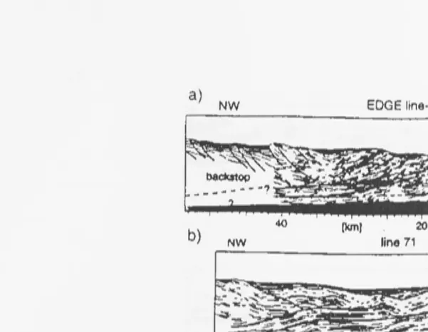
wedges include: the Alaskan (Figure 1.1), Nanaki, Oregon/Cascadia and Barbados accretionary

wedges [Gutscher et al, 1998b].

In regions of continental convergence, the crust is thicker (tens of kilometres) and the zone of

deformation is wider. Like sediments in an oceanic subduction zone, the upper crust is resistant to

subduction since it has a lower density than the lower crust and upper mantle [Tiflillett et al, 1993]. The upper crust is thus forced to detach from the subduct:i.ng lower mantle along a decollement

layer and mostly remains near the surface, while the lower crust and mantle lithosphere subducts.

As with accretionary wedges, the deformation is not uniform, but is localised along fault svstems .

(15)

a) NW EDGE line-302 SE

.---~--,-0

40

b) [kmJ 20 0

!kml

5

9

line 71 SE

,_..;..~---,0

NW

C} [km)

NW

:ore arc basin

40 _{ktnJ

20 0

(.kml

5

9

line 63 SE u

20 0

{luTI! 5

9

Figure 1.1: Various seismic reflection profiles of the Alaskan accretionary wedge, running from north ( a) to south ( c ). Scanned from Gutscher et al, [ 1998b ]. See this paper for the precise location of the profiles.

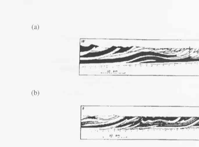
Similar to oceanic plate boundaries, crustal material builds up in compressional zones into wedge shaped orogens. Examples of these regions include Taiwan, the Canadian Rockies, the Appalachi-ans, etc. (see Figure 1.2). These zones are often called fold-and-thrust belts. Both accretionary wedges and fold-and-thrust belts are mechanically very similar (see [Dahlen, 1990]). The main difference between the two is scale: incoming oceanic crust/sediment is usually much thinner than the continental crust which enters a fold-and-thrust zone (typically 1km thick versus 30km thick).

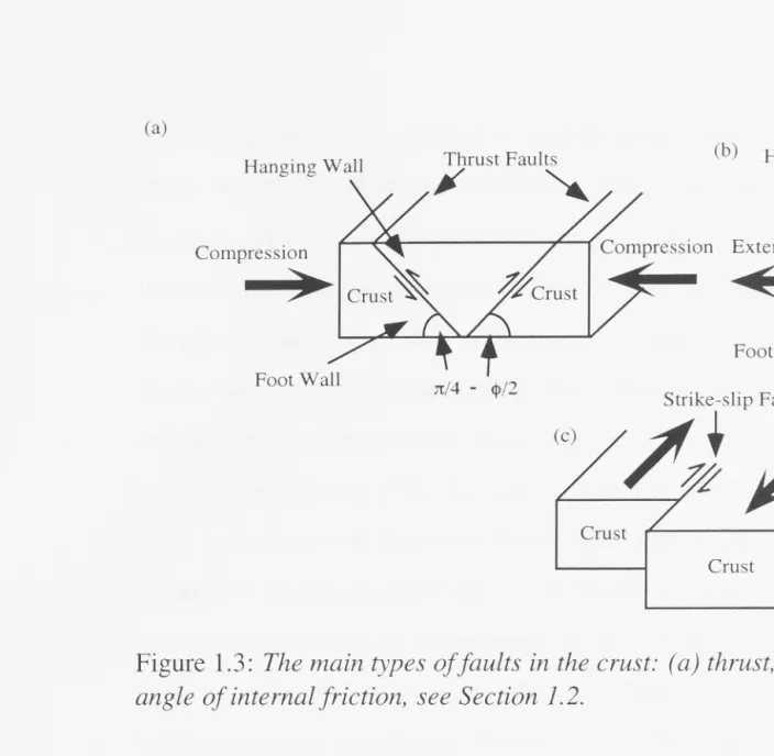
1.1.1 Types of Faults

Faults in the upper crust can be divided into three types: thrust, normal and strike-slip [Park,

[image:15.1206.54.655.91.556.2]

(16)

(a)

E

-

·-~-.!(! _ /cm_~ _{Canadian Rocf<.,e s}

(b)

E _w

-... ~-~ .;:_ -- _ ~ _ _

-- - .

-10 km

L . - - - , • .I _{Sourhern AiJO.:Jlac llians}

(c)

E · - ····- - - - -- -- ·- - -- - - -· - - ··· · - - ·

-w 1

T;iiwM

l _ __ _ _ ___,

.__-

_ __

··-~ - - - -- -·--·- ·- - - -- - ···--- --- -- - - - -- - - - . ·- . . . . __ _

Figure 1.2: A cross-section of typical fold-and-thrust belts ( a) Canadian Rockies, (b) Southern

Appalachians and ( c) Taiwan accretionary wedge. Scanned from [ Dahlen, 1990

J

and accommodate extensional deformation by "normal" movement (i.e. downward) of the

hang-ing wall block along the fault. Strike-slip faults are nearly vertical to accommodate displacement

parallel to the boundary between the plates.

Most plates do not have relative displacement which is either perfectly perpendicular or

paral-lel to the plate boundary. In fact, most boundaries are characterised by oblique relative

displace-ment of the plates with respect to the boundary. These zones can accommodate the deformation by

either forming oblique slip thrust/normal faults or by partitioning the strain onto two separate sets

of faults: one or more thrust faults which experience pure dip-slip (i.e. no strike- slip component)

and a strike-slip fault to accommodate the rest of the displacement (see Section 1.4.4).

Deeper down in the more ductile region of the crust, strain may not be so highly localised but

may be distributed into wide shear zones. This is supported by the observation that the pattern of

seismic reflectivity created by the faults often broadens out and disappears at depth and the lack

of substantial seismic activity in the lower crust [Ranalli, 1987].

[image:16.1206.39.724.103.608.2]

(17)

(a)

Hanging Wall Thrust Faults

~

"

Normal Faults

Compression

•

Compression Extension

Crust

•

Foot Wall

n/4 - qi/2 Jt/4 - qi/2

Crust

Figure 1.3: The main types of faults in the crust: ( a) thrust, (b) normal and ( c) strike-slip. <p is the angle of internal friction, see Section 1.2.

1.2 Mechanics of Crustal Faulting

Observed faults can be described to first order by assuming that the crust behaves like a Coulomb

material. This was first noted by Anderson who described the fault geometries in various locations

in Britain (see Anderson, [1951]). In a Coulomb material, failure occurs along a plane when the

shear stress at failure (TJ) is related to the normal stress across the fault plane (an) by

IT

J I = c

+

tan ¢ · an (1.1)

where c and ¢ are material constants known as the cohesion and the angle of internal friction, respectively. The coefficient of internal friction (µ) is given by

µ=tan¢ (1.2)

To first order, equation 1.1 holds for both the fracture of a brittle material (such as intact crustal

rock, [Paterson, 1978]) and for f1ictional slip along a pre-existing fault [Byerlee, 1978]. The main

difference between the two cases is the relative magnitude of the two terms. For frictional sliding

the first term is usually negligible when compared to the second term (see [Byerlee, 1978]). That

may not be the case for fracture of intact rock (see [Paterson, 1978]).

In can be shown (by using Mohr's incipient faulting theory, [Mandl, 1988]) that Coulomb's law

[image:17.1206.20.725.79.768.2]

(18)

of the maximum principal stress, o-_{1 ,}and lie in the plane whose normal is the intermediate principal

stress, o-_{2 .} If the orientation of the stress triad is uniform along the plate boundary, then all the

directions of slip coincide to form a straight fault plane [Burbidge & Braun, 1998]. Changes in

either the direction or magnitude of the principal stresses along a plate boundary will cause either

the type or direction of slip on the faults to change. If we assume that the principal stress triad

always has a vertical principal stress ( due to the weight of the overlying rock, sometimes called the

overburden) then the geometry of the three broad categories of faults can be shown to be consistent

with Coulomb theory (see [Turcotte & Schubert, 1982]). Oblique-slip faults can also be shown

to be consistent with Coulomb theory [Burbidge & Braun, 1998]. Burbidge & Braun, [1998]

argued that an oblique-slip fault can be thought of as an array of highly rotated thrust faults. This

was consistent with their experimental results which showed that the dip of the oblique-slip thrust

faults was related to the obliquity (the ratio of the strike-slip component of the convergence vector

to the convergent component, Section 1.4.4). They argued that the relation between the dip and

the obliquity was due to a rotation of the principal stress triad.

1.3 Mechanics of Accretionary Wedges

1.3.1 Introduction to Accretionary Wedges and Thrust Belts

During subduction, upper crustal material is removed from the subducting plate and accretes

against the over-riding plate. The interface between the accreting material and the over-riding

plate is known as the backstop, and is often modelled as a rigid wall (Section 4.1.1). There are two

broad modes of accretion [Platt, 1986]: the frontal accretion mode and the rear accretion mode

(Figure 1.4).

Frontal Accretion Mode

During frontal accretion the incoming sediment/upper crustal material is incorporated into the

wedge at the front of the prism. Deformation is accommodated by conjugate thrust fault pairs.

In many cases the pro-thrust faults (thrusts dipping towards the backstop, [Willett et al, (1993)])

accommodates more deformation than the retro-thrusts (thrusts dipping towards the toe).

Pro-thrusts can therefore be more clearly imaged by seismic methods. An example can be seen in

Figure 1. l(c). Frontal accretion has been observed in both analogue models (e.g. Davies et al,

[1983]) and in sections of a number of accretionary prisms/thrust belts (e.g. the Canadian Rockies,

(19)

(a)

Retro-Thrust

J

;ackstop

(b)

Backstop

Flat

I

....::::_

~

Underthrust Segment Ramp

Figure 1 .4: ( a) A schematic diagram of an accretionary wedge undergoing frontal accretion. In-coming upper crustal material is added to the front of the system by a pop-up structure which consists of a conjugate pair of thrust faults.

If

we use the naming convention of Willett et al, [ 1993 }, the conjugate pair consists of a pro-thrust (which dips to the right) and a retro-thrust fault (which dips to the left). (b) A schematic diagram of an accretionary wedge undergoing rear accretion. Material is underthrust beneath the wedge (perhaps by tens of kilometres) before being uplifted at the back. The dominant faulting system in this mode is a ramp-fiat ( or "staircase" fault structure). Normal faults near the crest of the prism are often observed in this mode.

the European Alps, the Oregon coast accretionary prism and the N ankai accretionary prism; see Platt, [1986] and references therein).

Rear Accretion Mode

[image:19.1206.79.729.54.617.2]

(20)

presence of metasomatised sediments near the rear of some prisms [Platt, 1986].

Mode Oscillation

Both of the two principal modes of accretion have been recently observed in a series of sandbox

experiments by Gutscher et al [1996, 1998a, 1998b]. Each mode has been observed separately

in other analogue models (e.g. Lui et al, [1992] and Cowan & Silling, [1978]). Gutscher et al,

[1998a,b] found that deformation in accretionary wedges can oscillate between frontal accretion

and rear accretion. As a result, the overall slope of the wedge also oscillates. In their experiments

they used two different basal frictions and found that frontal accretion occurs more often when

the basal friction is 0.35 than when it is 0.5. There is also evidence supporting an oscillation in

mode in a number of accretionary wedges (see Section 5.5.1). This oscillation can occur along the

strike of an accretionary wedge (compare Figure 1.l(a) and (b)). Alternatively, the same region

may change mode through time, (e.g. the Chugach Bay section of the Alaskan accretionary wedge

[Kusky et al, 1997]).

Extension in Accretionary Prisms

Another intriguing feature of accretionary wedges is the presence of normal faulting at the crest of

the prism, while the prism is undergoing compression [Willett, 1999a]. This is sometimes known

as syn-orogenic extension. Examples of this include Taiwan and the Variscan Orogen in Spain

[Willett, 1999a]. Syn-orogenic extension is often associated with the rear accretion mode [Platt,

1986].

Post-orogenic extension is also known and occurs after the tectonic compression which created

the mountain range or prism is removed. In this case, the horizontal principal stress decreases due

to the reduction of the tectonic stress component, while the vertical stress ( due to the weight of the

uplifted crust) remains the same. The strength of the orogen is insufficient to support the weight of

the thickened crust without the horizontal tectonic stress. Essentially, the orogen collapses under

its own weight. This may flatten mountain ranges faster than erosion processes alone [Malavielle,

1993].

Understanding Accretionary Prisms

To better understand the mechanics of accretionary prisms and thrust belts, we need to use some

form of model. There are three main methods for modelling upper crustal deformation: theoretical,

(21)

numerical and analogue. All three methods have their advantages and disadvantages. The previous

work in each of the three categories will now be described.

1.4 Theoretical Models of Convergent Upper Crustal Deformation

1.4.1 Early Models

Early this century, movement of thrust sheets were thought to be due to "gravity spreading or

gliding". However this explanation is difficult to reconcile with many observations from the field

[Chapple, 1978]. One of the first mechanical treatments was done by Elliot, [1976]. Elliot, [1976]

used the equilibrium equations and an a priori stress distribution within the wedge. He did not

incorporate the rheology of rocks into his formulation nor did he use a weak basal layer. His

analysis ignored shortening in the wedge material and indicated that a surface slope was necessary

for the formation of the wedge, but that a horizontal compressive force was not.

Chapple, [1978] assumed that the crust can be approximated as a perfectly plastic wedge (i.e.

a wedge where the strain rate is zero below a yield stress and arbitrary when the stress is equal to

the yield stress; stresses above the yield stress are not allowed). This particular choice of rheology

was arbitrary [ Chapple, 1978]. He pointed out that to be consistent with geological field data any

model must have

a.

thin-skinned deformation bounded below by an undeformed basement

b. a weak basal surface or detachment layer which dips towards the interior of the mountain

belt/wedge;

c. a large horizontal compression in the material above the detachment and,

d. a characteristic wedge shape.

Chapple, [1978] also observed that the internal deformation of the wedge required to

accommo-date shortening is some combination of folding and thrusting.

As with all theoretical models of accretionary wedges, Chapple, [1978] assumed that

con-tinuum mechanics theory can be applied to the wedge, despite the existence of faults within it.

Chapple, [1978] was also one of the first to assume that the material throughout the wedge was

undergoing yielding at all points in the wedge, rather than just along the faults within the wedge.

(22)

conditions, the stress and the velocities within the model. He also found that an initial surface slope is not necessary to create a fold and thrust belt, as is required in a gravity gliding model or

in the model by Elliot, [ 197 6].

1.4.2 Critical Taper Model

The next major advance in modelling the mechanics of accretionary wedges was done by Dahlen and colleagues in a series of papers which assumed that the wedge had a Coulomb rheology [Davis

et al., 1983; Dahlen 1984; Dahlen et al, 1984; Dahlen & Barr, 1989 and Dahlen, 1990]. As in

previous models, these papers all assume that the wedge is everywhere on the point of failure , i.e. that equation (1. 1) is true at every point in the wedge and that the wedge can be accurately modelled as a continuum. Dahlen, [1984] examined the case of a completely non-cohesive wedge (c

=

0) and Dahlen et al, [1984] examined the case with a non-zero cohesion. Davis et al, [1983] found that for a non-cohesive wedge the surface slope (a) is related to the basal slope ((3 ) by the relationship,

a

+

(3

=

'l/Jb - 'l/Jo

(1.3)

where

'l/Jb

is the angle of the direction of maximum compressive stress with respect to the base and

'l/Jo

is the same angle with respect to the surface. The sum of

a

and (3 is known as the taper of

the prism.

'l/Jb

and

'l/Jo

are functions of the internal and basal friction coefficients, the surface slope (a) and a "generalized" Hubbert-Rubey fluid pressure ratio (,,\) [Dahlen , 1990]. ,,\ is the ratio of pore fluid pressure to overburden stress [Hubert & Rubey, 1959], modified to include the case of a submarine wedge (see Dahlen, 1984). For the cohesionless wedge, Dahlen, [1984] derived an "exact" solution without having to assume a thin taper (i.e.

a+

(3

<<

l). However, Dahlen, [1984] did assume constant density (p ), µ and ,,\ throughout the wedge. The cohesionless wedge solution

of Dahlen, [1984] has also been derived using Mohr's circles [Lehner, 1986] and has been shown

to be the only possible solution to the problem consistent with the equations of static equilibrium for the given assumptions and boundary conditions [ Barcilon, 1987].

For a dry material on a weak base with a small taper, equation (1.3) can be approximated to (see [Dahlen, 1990]),

(23)

1 - sin¢

a

+

/J

~

.,

.

₁

({3

+

µb)

+

Sln

(1.4)

where ¢ is the angle of internal friction and µb is the coefficient of basal friction (µb

=

tan <Pb,

where <Pb is the angle of basal friction).

If cohesion is included in the model, the solution cannot be derived exactly since an integral

must be estimated by numerical quadrature [Dahlen, 1984]. However the non-cohesive wedge approximation is usually sufficient, since the overburden stress is usually much greater than the cohesion of crustal rocks or sediments in the majority of the wedge [Dahlen, 1984]. The only region where this may not be true is near the toe of the wedge where the wedge is thin and thus the overburden stress is small [Dahlen, 1984]. According to critical tapertheory, any cohesion in the material will cause the wedge surface to become concave [Dahlen et al, 1984]. A concave toe is found in a number of accretionary wedge profiles [Emmerman & Turcotte, 1983]. Approximate solutions for the cohesive wedge have also been found by Fletcher, [1989] and Stockmal, [1983] has looked at the problem using slip line theory.

The critical taper model has been extended to the case of a three-dimensional collision zone where the direction of convergence is oblique to the plate boundary (an oblique collision) [Platt,

1993, Koons, 1994, Enlow & Koons, 1998]. Spatially variable cohesion has been added to the model by Zhao et al, [1986]. Erosion and heat diffusion have also been added to Dahlen 's model

[Barr & Dahlen, 1989].

1.4.3 Viscous Models

Another family of accretionary wedge models assumes that the wedge has a viscous rheology.

(24)

(including Coulomb rheology) did not produce significant syn-orogenic extension.

1.4.4 Theoretical Models of Oblique Convergence

It has been observed that strain is partitioned in a number of different obliquely convergent

ac-cretionary wedges. Strain is partitioned when most of the strike-slip motion is accommodated by

strike-slip faults and most of the convergent motion is accommodated by thrust faults (e.g. Sunda

subduction zone in Indonesia [Fitch, 1972]). One of the earliest models on oblique convergence

was that by Fitch, [1972]. Fitch, [1972] showed that there was a critical angle at which total stress

along the non-partitioned system (oblique-slip thrust faults) and the partitioned system were equal.

He argued that oblique-slip faulting would proceed above this critical obliquity angle and that

par-titioning would occur below this angle. Beck, [1983] made a similar argument by assuming that

the faulting system which minimised the amount of energy dissipated in accommodating the

de-formation would be the preferred one. This argument could be used to incorporate viscous effects

if the faults penetrated into the mantle. Beck, [1991] later extended this to include the possibility

that slip on the thrust fault may be oblique-slip (rather than dip-slip, i.e. normal to the strike of

the fault). The assumption that the system will minimise the dissipated energy has been criticised

by some authors [Bird and Yuen, 1979], so McCaffrey, [1992] used the more "fundamental" force

balance equations to produce a relation for the critical obliquity angle. Other authors have also

produced relations for the critical obliquity angle directly from seismic data [Micheal, 1990 and

Walcott, 1978]. Platt, [1993] has extended critical taper theory to cover obliquely subducting

wedges. He also predicted a critical obliquity at which the wedge either moves with the backstop

or detaches from it.

All these models are best suited for regions of oceanic subduction against a rigid backstop

(which could be either the over-riding continental crust or previously lithified sediment). They all

treat the dip of the thrust faults as a given constant, independent of the obliquity. They also do

not include the possibility of mass flux of crustal material over the velocity discontinuity (i.e. the

backstop is infinitely high) and do not include the possibility that there may be faulting on both

sides of the strike-slip fault.

Burbidge & Braun, [1998] argued that the partitioning angle observed in their analogue models

occurs when the magnitude of the vertical principal stress equals one of the horizontal principal

stresses. This causes the maximum principal stress to change from being the vertical principal

stress to one of the horizontal principal stresses, i.e. the orientation of the stress triad changes

(25)

from one oriented for thrust faulting, to one oriented for strike-slip faulting. Their model does not

use a rigid backstop and has thrust faults on both sides of the strike-slip fault. This model is thus

more suitable for obliquely convergent continental settings.

1.4.5 Validity of the Models

Some authors have questioned the applicability of the various theoretical models of accretionary

wedge deformation to the real Earth. Some of the major problems include:

Viscosity

Viscous materials cannot support a shear stress without a corresponding strain rate. Thus the

ma-terial must be undergoing constant internal deformation (i.e. circulation) to maintain a slope. Yet

there are a number of old thrust belts/accretionary prisms where the system is inactive, but a slope

exists and is stable (e.g. the Canadian Rockies, [Chapple,1978]). The existence of such systems

is also a problem for the gravity-gliding models. In those models the slope causes deformation, so

there should not be inactive thrust belts or accretionary wedges with a slope [ Chapple, 1978].

Localisation

Thrust belts have highly localised deformation in both space and time. This leads to key

differ-ences between the mechanics of thrust belts and the critical taper theory [Bombolakis, 1994]. Both

the critical taper model (Section 1.4.2) and the viscous model (Section 1.4.3) require that

defor-mation occurs throughout the entire wedge. However, defordefor-mation in most accretionary prisms is

in fact concentrated along a limited number of faults. Furthermore, the required shortening

pre-dicted by the models near the back stop is not found near the back of certain thrust belts (e.g. the

Wyoming and Tennessee thrust belts, [Woodward, 1987]). The theories also require that the

me-chanical properties of the thrust belt are constant through time. However, the formation of faults

causes the effective coefficient of friction (µ) and/or cohesion (c) to decrease along those faults.

This causes localisation because deformation will preferentially occur where the material is

weak-est, as this will require the least amount of mechanical work [Masek & Duncan, 1998]. While

most critics have mainly focused on the applicability of the critical taper theory to thrust belts,

to a certain extent the problems also apply to accretionary wedges (since the deformation is also

localised deformation along faults in accretionary wedges [ Chapple , 1978]). In theoretical

(26)

in order to make the problem tractable, an assumption which may not be accurate.

The Complex Evolution of Accretionary Wedges

Thrust faults in accretionary wedges often display changes in (i) vergence (i.e. whether they dip

towards the toe or the backstop) and (ii) the location of maximum uplift. As has been mentioned

earlier, there are two principal modes of accretion in accretionary prisms: frontal and rear

accre-tion. Both produce different dominate vergence and different locations of maximum uplift. This

shows that the evolution of an accretionary wedge is more complex than the simple self-similar

growth predicted by theoretical models. There is also evidence of episodic behaviour (Section

1.3.1).

Syn-orogenic Extension

Syn-orogenic extension at the crest of accretionary prisms is another problem. It is quite

counter-intuitive that extension can occur simultaneously with compression in different parts of the prism.

Buck & Sokoutis, [1994] found that extension could occur at the crest of their viscous analogue

model. Willett, [1999a] also found extension in a viscous numerical model but not in models

with a Coulomb rheology. However, as argued earlier, Coulomb rheology is usually regarded as a

better model for the crust. The question is, can a model of the Earth based on a Coulomb rheology

reproduce the observed extension seen in the natural world?

1.5 Analogue Models of Crustal Deformation

1.5.1 Introduction to Analogue Models

Physical modelling of geological features has a long history going back over a century (see the

references in [Hubbert, 1951]). However, it was not until the seminal paper by Hubbert, [1937]

that physical modelling become properly scaled to the crust. In order to produce an experiment

that properly models crustal deformation, a material must be found which obeys a correctly scaled

version of equation ( 1.1).

According to Hubbert, [1951], the cohesion of the modelling material (cm) must be,

Cm= Cc Pm lm

Pc le

13

(27)

for the experiment to be correctly scaled to the crust. Cc is the cohesion of the crust, p is density

and l is a characteristic length scale (in this case the thickness of the layer). The subscript c refers

to the crust and m to the model. In order to make the experiment manageable, the dimensions of the model must be much smaller than the crust (e.g. modelling 5km of crust with a model

10cm high). If the density of the crust and model material are the same, then this means that one

must make the cohesion of the model material much smaller than that for the crust. Since the

effective cohesion of crustal rock is of the order of l0MPa, the correctly scaled cohesion of the

model material must be of the order of 100Pa. In order for the second term in the right hand side

of equation (1. 1) to scale, the coefficient of friction must be the same for both the model material

and the crust (since the coefficient of friction is dimensionless).

It has been known for some time that sand obeys equation (1. 1) over a wide range of stress

conditions (see [Lamb and Whitnian, 1968]). The angle of internal friction in dry sand is about the

same as that for crustal rock (29° - 40° for sand [Lambe and Whitman, 1968] and 27° - 39° for

crustal rock [Touloukian et al, 1989]). This correctly scales the second term in the right hand side

of equation (1.1) (see [Byerlee, 1978] and [Lambe and Whitnian, 1968]). The effective cohesion

is also of the correct order of magnitude for a crustal model (400 Pa [Kranz, 1991]). Basically,

sand can be used as a modelling material for the crust because both sand and crustal rock are

quasi-cohesionless Coulomb materials (i.e. the cohesion term in 1. 1 is dominated by the friction

term).

Sand grain size does not scale exactly to fault block size in the Earth. Thus features that depend

substantially on sand grain size and packing (such as fault zone width) do not scale properly

with the crust. The bulk elastic response of sand is also not correct for the crust [Mand!, 1988] ,

thus sand box models cannot be used to estimate how much convergence is required to reach a

given stage of deformation in natural accretionary wedges. Most sand box models also do not

incorporate the effect of fluid pressure on the deformation. Cobbold & Castro, [1999] suggest

pumping compressed air into sand to incorporate this effect, although this is yet to be used in any

analogue model at the time of writing. Cobbold & Castro, [1999] also give a fairly comprehensive

list of other sandbox models.

1.5.2 Early Analogue Models

Hubbert's Sandbox Experiment

(28)

mechanics. In this model, a box was filled with sand in alternating coloured horizontal layers.

A movable wall was placed in the middle of the box and slowly pulled along the length of the

box during an experiment. The sand on the right of the wall underwent an increase in horizontal

compressive stress, while the sand pack on the left of the wall underwent a decrease in the

hori-zontal compressive stress due to movement of the wall. A series of imbricate thrust faults formed

on the right side, while a normal fault formed on the left [Hubbert, 1951]. The dip of the faults

agreed very well with Anderson's theory of faulting in a Coulomb material. When applied to the

dynamics of convergent zones, this sort of model effectively assumes that there exists a horizontal

decollement between the upper crust and the upper mantle/lower crust and that the material on

the one side of the plate boundary is much stronger than the accreting sediment/upper crust on

the other side. This approximation works best for accretionary wedges where "soft" sediment is

accreted against stronger continental crust.

Other Early Experiments

One of the first analogue models to look at accretionary wedges was developed by Cowan & Silling

[1978]. They used wet clay and compared their result to the predictions of a viscous model. One

of the first models of normal faulting was developed by Horsfield, [1977] and one of the first on

oblique rifting experiments was done by Withjack & Ja,nison, [1986].

Critical Taper Sandbox Experiments

Davis et al, [1983] sand box experiments were conducted as experimental verification of critical

taper theory. The relationship between the average slope and basal dip agreed to within

exper-imental error with the theory for one particular set of basal and internal friction coefficients of

friction. No comparison was made between theory and experiment on the distribution of

deforma-tion within the wedge.

1.5.3 Malavielle's Sandbox Experiment

Malavielle , [1984] lifted the rigid backstop assumption by shifting the basal velocity discontinuity

from the comer of the box near the wall, to the centre of the box. Instead of moving the wall, he

pulled a piece of cloth along the base of the sand pack and down a slit in the middle of the box.

The slit is fixed relative to one side of the sand pack (the one which is not above the moving piece

of cloth). This gives an asymmetric basal velocity and hence an asymmetric faulting distribution.

(29)

As the cloth is pulled down through the slit, an increasing number of thrust faults form above the moving sheet and a single narrower zone of faulting forms within the sandpack above the stationary sheet. The side of the basal discontinuity above the moving sheet was later named the "pro-side" and the faults "pro-thrusts" by Willett et al, [1993]. The other side of the pack was similarly termed "retro-side" and the faults, "retro-thrusts". This kind of model is appropriate for continental collision zones where there is no great strength contrast across the plate boundary and thus no reason to invoke the presence of a rigid backstop. After large amounts of deformation, a wedge with a relatively shallow slope forms on the pro-side and a more steeply sloping wedge forms on the retro-side. It has been argued that the pro-side and retro-side wedges correspond to the two extreme solutions to the critical taper model derived by Dahlen, [1990]. The shallow pro-side wedge corresponds to a wedge at the critical taper which has benn formed by compression, while the steep retro-side wedge is the critical taper formed by extension [Willett et al, 1993].

1.5.4 Miscellaneous 2-D Accretionary Wedge Experiments

Koons, [1990], used a small rigid wall to allow sand to flow over the backstop. This created a two-sided orogen model similar in structure to the accretionary wedge in the experiment by Malavielle,

[1984]. One of the first tomographic analysis on an analogue model was done by Colletta et al,

[ 1991]. The effect of different backstops in a rigid backstop experiment has been investigated by Byrne et al, [1993]. The effect of changes in the amount of overburden on the pattern of faults has been examined by Marshak & Wilkerson, [1992]. Sarti et al, [1997] used finely layered models to systematically examine folding in accretionary wedges. The effect of sedimentation on critical taper models was examined by Sarti & McClay, [1995]. Sandbox experiments have been compared to the Peruvian margin with good results by Kukowski et al, [1994]. A four layer model (down to the mantle) has been done by Davy & Cobbold, [1991]. Shemenda, [1994] has conducted a wide range of two layer (i.e. brittle crust and viscous mantle) models of subduction. Sandbox models with alternating brittle and viscous layers (e.g. silicone putty) have been done by

Verschuren et al, [1996]. Curved fault structures (in plan view) have been investigated by Marshak

et al, [1992]. The three-dimensional structure of thrust faults was examined by Mulugeta & Koyi,

(30)

under accretionary wedges using sandbox models. The effect of a dipping in den tor ( or backstop) has been investigated by Bonini etal, [1999].

1.5.5 Miscellaneous Extensional, Strike-Slip or Obliquely Convergent Experiments

Normal faults in extensional regimes have been modelled by: [Richard, 1991; Higgs & McClay,

1993; Braun et al, 1994; Hauge & Gray, 1996; Brune & Ellis, 1997; Hatzfeld et al, 1997; Rahe et

al, 1998; Nieuwland & Walters, 1993; Tron & Brun, 1991]. A simplified extensional experiment has been done by Boerner & Sclater, [1992] using hexagonally packed steel balls with uniform radius. Pure strike-slip faults have been modelled using sand by Schreurs, [1994], Naylor et al,

[1986], and Dauteuil & Mart, [1998]. Early analogue models such as Riedel, [1929] and Cloos,

[1928] used clay-cake models.

1.5.6 Obliquely Convergent Experiments

Oblique-slip faults created by motion along the basement have been modelled in a number of experiments. Richard, [1991] used a box split down the middle and filled with sand. Richard,

[1991] simultaneously lifted one half of the experimental table while moving it horizontally to give either oblique convergence or rifting ( depending on the direction of the horizontal motion).

In the experiment, Richard, [1991] found two thrust faults formed with a large dip when there was obliquely convergent motion. The deformation was thus accommodated without partitioning. For divergent oblique slip, two normal faults formed on both sides of the basement fault and a strike-slip fault formed directly above the basement fault, i.e. the strain was partitioned. The addition of a silicone layer between the sand and the table (to simulate a viscous upper mantle) generally reduced the number of faults seen at the surface.

Richard and Cobbold, [1989] have also tried to model obliquely convergent basement faults. Their model was similar to Richard, [1991] except that instead of lifting half of the table they pulled two plastic sheets through the gap between the two halves of the table to simulate the

convergent component of the convergence. They also compressed the sand pack from the sides with two pistons. Their results indicate that when strike-slip predominates over convergent motion (low obliquity) the thrust faults produced are on average more steeply dipping. The addition of

a viscous layer beneath the sand "encourages" partitioning. Molnar, [1992] believes this is due to the viscous silicone "smoothing" out the relative displacement and so allowing partitioning.

Pinet & Cobbold, [1992] conducted elaborate multi-layer models of the Phillipine subduction

(31)

zone with both lateral and vertical inhomogeneities. They compressed their rectangular model by moving the back wall and one of the side walls along the box. They found that very large changes in the thickness of the experiment could have an observable effect on the faults produced. These large differences could only be expected to occur at collisions between oceanic lithosphere and continental lithosphere, or those involving narrow island arcs. Burbidge & Braun, [1998] conducted a range of different obliquely convergent sandbox experiments. They found that there was a critical obliquity for partitioning to occur. A full lithosphere model (similar to those done by

Shenienda, [ _{1994]) of oblique convergence has been done by}_{Chemenda et al,}_{[2000]. They found}

that the degree of partitioning depends on the strength of the coupling between the over-riding and subducting plate.

Obliquely convergent zones have also been examined by [Pinet & Cobbold, 1992; Wilkerson et al, 1992; Koons & Henderson, 1995; Haq & Davis, 1997; Chemenda et al, 1997; Norris & Cooper, 1995; Lu & Malavielle, 1994; Norris et al, 1990; Bonini, 1998; Corrado et al, 1998].

1.5.7 Differences with Coulomb Theory

Mulugeta, _{[1988] compared the results of sandbox experiments to the predictions of Coulomb}

theory. They noted that the wedge continues changing its surface slope throughout the experi-ment. This is contrary to Coulomb wedge theory which predicts that the wedge should build up in surface slope to a minimum stable taper angle, and then maintain this angle for continued defor-mation. Similar results were found by Gutscher et al, [1996] for large deformation experiments. They found that the mean surface slope oscillated through the experiment, the effect being more pronounced with larger values of basal friction. Koyi, _{[1995] also noted that the wedge does not}

grow self-similarly but episodically.

The pro- and retro-wedges have also been shown to stabilize at different angles than predicted by critical taper theory, particularly for basal friction experiments substantially different ( either higher or lower) from that for mylar (a type of drafting film, µba se ~ 0.3) _{[Wang & Davis,}_1996;

Lui et al 1992]. Mulugeta, _{[1998] also found that the dip of the faults they observed were not}

(32)

comparison with critical taper theory would be achieved if the experiment was started with a flat

sand pack and then allowed to build up to the (theoretically) minimum critical taper. It would be

interesting to see what relationship between this slope and the basal friction actually is. This has

not been done, since it is difficult to find a variety of suitable basal materials. It would also be

interesting to examine the effect of changing the internal friction on the slope formed. However,

only sand has ever been used in these experiments and it is difficult to find sand types with highly

variable internal friction coefficients.

Critical taper theory also implies a continuous distribution of faults, while real accretionary

wedges (in both the sandbox and in the field) exhibit highly localised deformation along a limited

number of faults. Sassi et al, [1993] tested the effect of pre-existing faults by cutting a sandpack

with a piece of wire before conducting the experiment. Even this relatively small weakening of

the material (approximately 7% reduction in friction [Kranz, 1991]) caused a change in behaviour,

as the faults were located preferentially along the pre-existing zones of weakness. In real wedges,

the difference between faults and intact rock would probably be even greater, highlighting the

importance of the fractured nature of the crust.

1.6 Continuum Numerical Models of Continental Deformation

1.6.1 Finite Element Method (FEM) Models

The other major avenue of research into accretionary wedges/thrust belts dynamics is numerical

modelling. Numerical models do not require as many assumptions as analytical models and allow

a greater variation and control of parameters than do analogue models. Most numerical

meth-ods have used some type of Finite Element Method (FEM) technique. By dividing the material

into elements, the equations of force balance can be reduced to solving a set of linear algebraic

equations which can be used to obtain an approximation of stress and strain in the system [Bathe,

1982]. The FEM implies that properties such as nodal displacement and velocity are continuous

across the elements, i.e. throughout the model. This means that FEM models often have

diffi-culty in modelling highly localised deformation as seen in accretionary wedges. Large amounts

of deformation leads to mesh deformation and error in the calculation. Since the deformation is

highly localised along fault zones, these regions can become highly deformed very quickly, which

rapidly produces problems in the calculation. FEM models are therefore often limited to relatively

small amounts of deformation. While many of these models show localised strain rate, it should

(33)

be remembered that faults are zones of localised total strain. Only if the zone of strain rate remains fixed in the material will the two be the same. If the zone of strain rate moves steadily through the material, a distributed zone of strain will be formed. This is particularly noticeable in most

models of the pro-side of an accretionary wedge. The distributed nature of the strain makes it

difficult to infer the geometry of geological structures (such as faults) from FEM models of

ac-cretionary wedges or fold-and-thrust belts. The latest FEM are much more capable of modelling

faults, although most of them are yet to be published (C. Beaumont, pers. comm.).

1.6.2 Accretionary Wedge Finite Element Models

One of the earliest attempts to model a Coulomb wedge numerically was by Willett [1992]. His

model did not incorporate an elastic component, had a flat base

(/3

=

0°) and a rigid, frictionless, vertical backstop. Wedges were produced with a parabolic cross-section and a different dip than

predicted by critical taper theory. This was attributed to the frictionless backstop. Strain within

the wedge was distributed.

Makel & Walters _{[1993] produced a finite-element model which showed localisation of the}

strain rate. However, they were limited to very small amounts of deformation. Once the first fault

formed in the model the calculation had to be halted. In Makel & Walter, [1993] the initial zones

of localised strain rate were similar in their geometry to the first faults formed in a sandbox with

similar boundary conditions.

One FEM which produced localised total plastic strain is that by [Sassi & Faure, 1997] . In

this paper they displayed unpublished data based on a model by Plischke [1991]. The plots of

plastic strain show similar results to the faults seen in sandbox models for relative large amounts

of deformation. The model assumes an elasto-plastic behaviour with a Drucker-Prager criterion,

friction hardening-softening and cohesion softening flow rules. Faults were modelled by inserting

an internal boundary when a shear band traversed the entire layer thickness. Thus, faults do not

emerge dynamically.

Miscellaneous FEM Models

Willett, _{[1992] performed a numerical simulation similar to}_{Malavielle's,}_{[1984] sandbox}

experi-ment. The overall cross-section was similar to Malavielle's, [1984] experiment, but the geometry

of faults were difficult to extract from the model. In the model by Willett et al [1993], the

(34)

occur in all sandbox models (e.g. [Wang & Davis, 1996]). A similar model was done by Braun

& Sambridge, _{[1994] using the Dynamic Lagrangian Remeshing (DLR) method.} _{Beaumont et}

al _{[1994] also conducted a similar experiment using a thermally-activated, depth dependent}

rhe-ology, a situation which is difficult to model with sandbox experiments. Beaumont & Quinlan

[ 1994] looked at a variety of rheologies and boundary conditions. Later numerical work

concen-trated on extending the analysis to three-dimensions (e.g. [Braun & Beaumont, 1995] ) and on the

effect of one pre-existing fault (e.g. [Van Wees et al, 1996]). Hassani et al [1997] modelled the

case where virtually all the crust is subducted (a "non-accretionary" subduction zone [Lalle,nand

et al, 1994]).

Other models have looked at fluid flow in orogens ([Koons et al, 1998] and fault slip along a

pre-existing fault or set of faults ([Fugelso & Marshall, 1989] & [Oglesby et al, 1998]). The most

recent models have included the lower crust and upper mantle in full lithosphere models of crustal

convergence, (e.g. Ellis et al [1999] and Beaumont et al, [1999]). A variety of rheological models

have been modelled by Willett, [1999a], in an attempt to find the rheology which produces

syn-orogenic extension near the top of the orogen. The phenomena has been observed in numerous

localities, most notably Taiwan. Willett, _{[1999b] has also conducted full lithosphere models which}

includes the effect of erosion.

1.7 Distinct Element Models

Discontinuum models of crustal deformation have a shorter history than FEM models. The most

common type of discontinuum model is the distinct element model (DEM), initially developed by

Cundall & Strack, _{[1979]. In DEM the material is divided into discrete elements. Each element}

then interacts with the neighbouring elements with which it is in contact. This interaction is usually

represented by some sort of elastic-frictional relationship. The elements are allowed to separate

from each other and thus new contacts are allowed to form and break. It is this geometrical

flexibility that makes DEM different from FEM, in which neighbouring elements are not allowed

to separate and nodal displacements must be continuous across element boundaries.

Strictly, the term discrete _{element method is any method which has the following properties}

[Cundall & Hart, 1989]:

1. allows finite displacement and rotations of discrete bodies, including complete detachment,

and

The complex evolution of accretionary wedges and thrust belts : results from numerical experiments using the distinct element method