A Probabilistic, Distributed, Recursive Mechanism for Decision-making in the Brain

Decision-making in the Brain

.

White Rose Research Online URL for this paper:

http://eprints.whiterose.ac.uk/127628/

Version: Published Version

Article:

Caballero, J., Humphries, M.D. and Gurney, K. orcid.org/0000-0003-4771-728X (2018) A

Probabilistic, Distributed, Recursive Mechanism for Decision-making in the Brain. PLoS

Computational Biology, 14 (4). e1006033. ISSN 1553-734X

https://doi.org/10.1371/journal.pcbi.1006033

[email protected] https://eprints.whiterose.ac.uk/ Reuse

This article is distributed under the terms of the Creative Commons Attribution (CC BY) licence. This licence allows you to distribute, remix, tweak, and build upon the work, even commercially, as long as you credit the authors for the original work. More information and the full terms of the licence here:

https://creativecommons.org/licenses/

Takedown

If you consider content in White Rose Research Online to be in breach of UK law, please notify us by

A probabilistic, distributed, recursive

mechanism for decision-making in the brain

Javier A. Caballero1,2*, Mark D. Humphries1‡, Kevin N. Gurney2‡

1Faculty of Biology, Medicine and Health, University of Manchester, Manchester, United Kingdom, 2Deptartment of Psychology, The University of Sheffield, Sheffield, United Kingdom

‡ These authors are joint senior authors on this work. *[email protected]

Abstract

Decision formation recruits many brain regions, but the procedure they jointly execute is unknown. Here we characterize its essential composition, using as a framework a novel recursive Bayesian algorithm that makes decisions based on spike-trains with the statistics of those in sensory cortex (MT). Using it to simulate the random-dot-motion task, we demon-strate it quantitatively replicates the choice behaviour of monkeys, whilst predicting losses of otherwise usable information from MT. Its architecture maps to the recurrent cortico-basal-ganglia-thalamo-cortical loops, whose components are all implicated in decision-mak-ing. We show that the dynamics of its mapped computations match those of neural activity in the sensorimotor cortex and striatum during decisions, and forecast those of basal ganglia output and thalamus. This also predicts which aspects of neural dynamics are and are not part of inference. Our single-equation algorithm is probabilistic, distributed, recursive, and parallel. Its success at capturing anatomy, behaviour, and electrophysiology suggests that the mechanism implemented by the brain has these same characteristics.

Author summary

Decision-making is central to cognition. Abnormally-formed decisions characterize dis-orders like over-eating, Parkinson’s and Huntington’s diseases, OCD, addiction, and com-pulsive gambling. Yet, a unified account of decision-making has, hitherto, remained elusive. Here we show the essential composition of the brain’s decision mechanism by matching experimental data from monkeys making decisions, to the knowable function of a novel statistical inference algorithm. Our algorithm maps onto the large-scale architec-ture of decision circuits in the primate brain, replicating the monkeys’ choice behaviour and the dynamics of the neural activity that accompany it. Validated in this way, our algo-rithm establishes a basic framework for understanding the mechanistic ingredients of decision-making in the brain, and thereby, a basic platform for understanding how pathologies arise from abnormal function.

a1111111111 a1111111111 a1111111111 a1111111111 a1111111111 OPEN ACCESS

Citation:Caballero JA, Humphries MD, Gurney KN (2018) A probabilistic, distributed, recursive mechanism for decision-making in the brain. PLoS Comput Biol 14(4): e1006033.https://doi.org/ 10.1371/journal.pcbi.1006033

Editor:Jean Daunizeau, Brain and Spine Institute (ICM), FRANCE

Received:October 31, 2016 Accepted:February 12, 2018 Published:April 3, 2018

Copyright:©2018 Caballero et al. This is an open access article distributed under the terms of the

Creative Commons Attribution License, which permits unrestricted use, distribution, and reproduction in any medium, provided the original author and source are credited.

Data Availability Statement:Data from sensory cortex are available within the paper and from

http://www.neuralsignal.org/index_data.htmlwithin the Macaque database via accession number nsa2004.1. Third-party behavioural and neural data from sensorimotor cortex and striatum is not owned by the authors. However, it is available upon request to Anne Churchland (churchland@cshl. edu) and Long Ding ([email protected]), respectively.

Introduction

Decisions rely on evidence that is collected for, accumulated about, and contrasted between available options. Neural activity consistent with evidence accumulation over time has been reported in parietal and frontal sensorimotor cortex [1–5], and in the subcortical striatum [6,

7]. What overall computation underlies these local snapshots, and how it is distributed across cortical and subcortical circuits, is unknown.

Multiple models of decision making match aspects of recorded choice behaviour, associated neural activity or both [8–16]. While successful, they lack insight into the underlying decision mechanism. In contrast, other studies have shown how exact inference algorithms may be plausibly implemented by a range of neural circuits [17–21]; however, none of these has repro-duced experimental decision data.

Here we test the hypothesis that the brain implements an approximation to an exact infer-ence algorithm for decision making. We show that the algorithm reproduces behaviour quan-titatively while the dynamics of its inner variables match those of corresponding neural signals on the random dot motion task—a highly developed paradigm to probe decision formation. By doing so, we predict how experimentally-acquired snapshots of neural activity map onto inference operations. We show this mapping accounts for the involvement of full recurrent cortico-subcortical loops in decision making. Evidence accumulation is thus predicted to occur over the entire loops, not just within cortex. Introducing this algorithm enables us to predict which aspects of neural activity are necessary for inference—hence decision-making— and which are not. For instance, recent data questioned whether non-increasing cortical firing rates encode evidence accumulation during decisions [22,23]. We demonstrate that, counter-intuitively, non-increasing as well as increasing cortical rates can encode likelihood functions, and hence evidence accumulation.

Our algorithm explains the decision-correlated experimental data more comprehensively than any prior model, thus introducing a new, cohesive formal framework to interpret it. Col-lectively, our analyses and simulations indicate that mammalian decision-making is imple-mented as a probabilistic, recursive, parallel procedure distributed across the cortico-basal-ganglia-thalamo-cortical loops.

Results

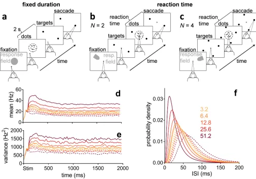
We tested our algorithm against behavioural and electrophysiological data recorded in sensori-motor cortex [3] and striatum [6], from monkeys performing 2- and 4-alternative reaction-time versions of the random dot motion task (Fig 1b and 1c). The decision evidence for the algorithm also simulates spike-trains from sensory cortex (the area that provides evidence to sensorimotor cortex), whose statistics we extracted from a third random-dot-task data set by [24]. In all forms of the task, the monkey observes the motion of dots and indicates the domi-nant direction of motion with a saccadic eye movement to a target in that direction. Task diffi-culty is controlled by the coherence of the motion: the percentage of dots moving in the target’s direction.

During the dot motion task, neurons in the middle-temporal visual area (MT) respond more vigorously to visual stimuli moving in their “preferred” direction than in the opposite “null” direction [24]. Both the mean (Fig 1d) and variance (Fig 1e) of their response are pro-portional to the coherence of the motion (see alsoS4 Fig). MT responses are thence assumed to be the uncertain evidence upon which a choice is made in this task [1,9].

www.conacyt.gob.mx) Fellowship (JAC), a Medical Research Council Senior non-Clinical Fellowship (MDH; MR/J008648/1;www.mrc.ac.uk), and a Wellcome Trust collaborative research award (JAC, MDH; 105610/Z/14/Z;www.wellcome.ac.uk). The funders had no role in study design, data collection and analysis, decision to publish, or preparation of the manuscript.

Recursive MSPRT

Normative algorithms are useful benchmarks to test how well the brain approximates an opti-mal probabilistic computation. The family of the multi-hypothesis sequential probability ratio test (MSPRT) [25] is an attractive normative framework for understanding decision-making. However, the MSPRT is a feedforward algorithm. It cannot account for the ubiquitous pres-ence of feedback in neural circuits and, as we show ahead, for slow dynamics in neural activity that result from this recurrence during decisions. To solve this, we introduce a novel recursive generalization, the rMSPRT, which uses a generalized, feedback form of the Bayes’ rule we deduced here from first principles (Eq 5).

We now conceptually review the MSPRT and introduce the rMSPRT (Fig 2), giving full mathematical definitions and deductions in theMaterials and methods. The (r)MSPRT decides which ofNparallel, competing alternatives (or hypotheses) is the best choice, based on

Csequentially sampled streams of evidence (or data). For modelling the dot-motion task, we haveN= 2 orN= 4 hypotheses—the possible saccades to available targets (Fig 1b and 1c)—

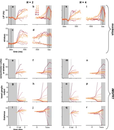
Fig 1. Random dot motion task and statistics of neural responses in sensory cortex (MT).(a) Fixed duration task for MT recordings [24]. (b, c) Reaction time task for sensorimotor cortex and striatum recordings,N= 2, 4 alternatives [3,6]. (d, e) Smoothed population moving mean and variance of the firing rate of MT during the fixed duration dot motion task (189–213 neurons), aligned at onset of the dot stimulus (Stim), for a variety of coherence percentages (colour-coded as in the legend in panel f). Solid lines are statistics when dots were moving in the preferred direction of the MT neuron. Dashed lines are statistics when dots were moving in the opposite, null direction. Data from [24], re-analysed. (f) Lognormal density functions for the inter-spike intervals (ISI) specified by the statistics over the approximately stationary segment of (d, e) before smoothing (parameter setOinTable 1). Preferred and null motion directions by line type as in (d, e).

and theCuncertainevidence streamsare assumed to be simultaneous spike-trains produced by visual-motion-sensitive MT neurons [1,9] (seeMethods). Every time new evidence arrives, the (r)MSPRT refreshes ‘on-line’ the likelihood of each hypothesis: the plausibility of the com-bined evidence streams assuming that hypothesis is true. The likelihood is then multiplied by the probability of that hypothesis based on past experience (the prior). This product for every hypothesis is then normalized by the sum of the products from allNhypotheses; normalisation is crucial for decision, as it provides the competition between hypotheses. The result is the probability of each hypothesis given current evidence (the posterior)—adecision variableper hypothesis. Finally, posteriors are compared to a threshold, whose position controls the speed-accuracy trade-off. A decision is then made to either choose the most probable hypothesis, if its posterior surpassed the threshold, or to continue sampling the evidence streams otherwise. Crucially, the (r)MSPRT allows us to use the same algorithm irrespective of the number of alternatives, and thus aim at a unified explanation of theN= 2 andN= 4 dot-motion task variants.

The MSPRT is a special case of the rMSPRT (in its general form in Eqs5and10) when pri-ors do not change or, equivalently, for an infinite recursion delay; that is,Δ! 1. Also, the previous recurrent extension of MSPRT [18,26] is a special case of the rMSPRT whenΔ= 1. Hence, our rMSPRT generalizes both in allowing the re-use of posteriors fromanygiven time in the past as priors for present inference. This uniquely allows us to map the rMSPRT onto neural circuits containing arbitrary feedback delays, in particular solving the problem of decomposing the decision-making algorithm into distributed components across multiple brain regions. We show below how this allows us to map the rMSPRT onto the cortico-basal-ganglia-thalamo-cortical loops.

Inference using recursive and non-recursive forms of Bayes’ rule gives the same results (e.g.

see [27]), and so MSPRT and rMSPRT perform identically. Thus, like MSPRT [17,25], for

N= 2 rMSPRT also collapses to the sequential probability ratio test of [28]; the rMSPRT is

Fig 2. The MSPRT and rMSPRT as a diagram.Circles joined by arrows are the Bayes’ rule. AllCevidence streams (data) are used to compute every one of theNlikelihood functions. The product of the likelihood and prior probability of every hypothesis is normalized by the sum (∑) of all products of likelihoods and priors, to produce the posterior probability of that hypothesis. All posteriors are then compared to a constant threshold. A decision is made every time with two possible outcomes: if a posterior reached the threshold, the hypothesis with the highest posterior is picked, otherwise, sampling from the evidence streams continues. The MSPRT as in [25] and [17] only requires what is shown in black. The general recursive MSPRT introduced here re-uses the posteriorsΔtime steps in the past for present inference, thus re-using itself; hence the rMSPRT is shown in black and blue. If we are to work with the negative-logarithm of the Bayes’ rule—as we do in this article—all relations between computations are preserved, but products of computations become additions of their logarithms and the divisions for normalization become their negative logarithm.Eq 9shows this for the rMSPRT. The rMSPRT itself is formalized byEq 10.

thereby optimal, not only in the oft-used sense of using all available information to do statisti-cal inference (e.g.using the Bayes’ rule), but also in the strict sense that it requires the smallest expected number of observations, thus the shortest time to decide, at any given error rate (which follows from [29]). This is to say that the (r)MSPRT is quasi-Bayesian in general: the physical limit of performance or ideal Bayesian observer for two-alternative decisions (N= 2), and an asymptotic approximation to it for decisions between more than two (N>2) (which follows from [17,25]).

Upper bounds of decision time predicted by the (r)MSPRT

The hypothesis that the brain approximates an exact inference algorithm during decision for-mation is so far untested. This requires showing how uncertain sensory spike-trains can be transformed into the experimentally recorded choices. We do so here for the first time by com-paring the predicted choice reaction times of the (r)MSPRT to those of monkeys performing the random dot motion task. We sought to account for the reaction time dependence on three factors: the coherence of the dot motion, the number of decision alternatives, and the trial’s outcome (error, correct). We use a particular instance of rMSPRT (Eqs9and10) to determine predicted normative bounds on the decision time in the dot motion task. We can then ask how well monkeys approximate such bounds. The bounds result from using a minimal amount of sensory information, by assuming as many evidence streams (spike-trains from MT neurons) as alternatives; that is,C=N. Thus, this rMSPRT instance gives the upper bound on optimal expected decision times (exact forN= 2 alternatives, approximate forN= 4) per con-dition(given combination of coherence andN). AssumingC>Nwould predict even shorter optimal expected decision times (see [20]).

We assume that during the random dot motion task (Fig 1a–1c), the evidence streams for every possible saccade come as simultaneous sequences of inter-spike intervals (ISI) produced in MT. On each time step, fresh evidence is drawn from the appropriate (null or preferred direction; seeMethods) ISI distributions extracted from MT data (Fig 1f). By repeating the simulations for thousands of trials per condition, we can compare algorithm and monkey performance.

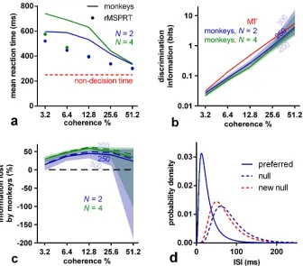
Using these data-determined MT statistics, the (r)MSPRT predicts that the mean decision time on the dot motion task is a decreasing function of coherence (Fig 3a). For comparison with monkey reaction times, the algorithm’s reaction times are the sum of its decision times and estimated non-decision time, encompassing sensory delays and motor execution. For macaques 200–300 ms of non-decision time is a plausible range [30,31]. Within this range, monkeys tend not to reach the predicted upper bound of reaction time (Fig 3a).

The monkey brain loses otherwise useful information from sensory

evidence

require to obtain the same reaction times on correct trials as the monkeys, per condition. We thus find, first, that the discrimination information available for decision is very similar across

N(Fig 3b), implying that monkeys use MT sensory information consistently. Second, and most important, we find that monkeys tended to use less discrimination information than that in ISI distributions in their MT when making the decision. In contrast, the (r)MSPRT uses the full discrimination information available. This implies that the decision-making mechanism in the monkey brain lost large proportions of MT discrimination information (Fig 3c). Since these (r)MSPRT decision times are upper bounds, this in turn means that this loss of discrimi-nation information in monkeys (Fig 3c) is the minimum.

Fig 3. (r)MSPRT predicts information loss during decision making.(a) Comparison of the mean reaction time of monkeys for 2 and 4 alternatives (lines) with that predicted by (r)MSPRT (markers), both for correct trials. Red line: assumed 250 ms of non-decision time. Simulation values are means over 100 Monte Carlo experiments each comprising 3200, 4800 total trials forN= 2, 4, correspondingly, under the parameter setO_{extracted from MT} recordings. (b) Discrimination information per ISI in MT statistics (red) compared to the (r)MSPRT’s predictions of the discrimination information available to the monkeys (blue, green). Central lines are for a non-decision time of 250 ms; the edges of the correspondingly-coloured shaded regions are for non-decision times of 300 and 200 ms. (c) As per panel (b), but expressed as a percentage of information lost by monkeys with respect to the information available in MT for the three assumed non-decision times (solid lines and shadings). The information lost if the reaction time match is further enhanced is shown as dashed lines (assuming 250 ms of non-decision time; seeMethods). (d) Example ISI density functions before (blue) and after (solid blue and dashed red) information depletion;N= 2, 51.2% coherence, and 250 ms of non-decision time. The null distribution was adjusted to become the ‘new null’ by changing its mean and standard deviation to make it more similar to the preferred distribution. Once done throughout and for a non-decision time of 250 ms, this procedure gives ISI distributions bearing a reduced amount of discrimination information (blue or green lines in panel b), rather than the full discrimination information actually produced by MT (red line). That is, after adjustment, the discrimination information between the preferred and ‘new null’ distributions matches that estimated from the monkeys’ performance.

(r)MSPRT with depleted information quantitatively reproduces monkey

performance

To verify if this information loss alone could account for the monkeys’ deviation from the (r)MSPRT upper bounds, we depleted the discrimination information of its input distributions to exactly match the estimated monkey loss inFig 3cper condition. We did so only by modify-ing the mean and standard deviation of the null direction ISI distribution, to make it more similar to the preferred distribution (exemplified inFig 3d).

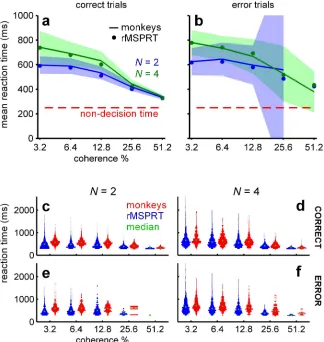
Using these information-depleted statistics, the mean reaction times predicted by the (r)MSPRT in correct trials closely match those of monkeys (Fig 4a). Importantly, this involved

noparameter fitting. Instead, we used the fact that for (r)MSPRT the mean total information for a decision is constant given error rate andN; this implies that longer decision times could only result from reducing the discrimination information in the evidence. Strikingly, although this information-depletion procedure is based only on data from correct trials, the (r)MSPRT

Fig 4. Monkey reaction times are consistent with (r)MSPRT using depleted discrimination information.(a, b) Mean reaction time of monkeys (lines) with 99% Chebyshev confidence intervals (shading) and (r)MSPRT predictions for correct (a;Eq 14) and error trials (b;Eq 15) when using information-depleted statistics (MT parameter setO_{d). (r)} MSPRT results are means of 100 simulations with 3200, 4800 total trials each forN= 2, 4, respectively. Confidence intervals become larger in error trials because monkeys made fewer mistakes for higher coherence levels. (c-f) ‘Violin’ plots of reaction time distributions (vertically plotted histograms reflected about the y-axis) from monkeys (red; 766– 785, 1170–1217 total trials forN= 2, 4, respectively) and (r)MSPRT when using information-depleted statistics (blue; single Monte Carlo simulation with 800, 1200 total trials forN= 2, 4).

now also matches closely the mean reaction times of monkeys from error trials (Fig 4b), which are consistently longer than those of correct trials (S1 Fig). Moreover, for both correct and error trials the (r)MSPRT accurately captures the relative scaling of mean reaction time by the number of alternatives (Fig 4a and 4b).

The reaction time distributions of the algorithm closely resemble those of monkeys in that they are positively skewed and exhibit shorter right tails for higher coherence levels (Fig 4c– 4f). These qualitative features are captured across both correct and error trials, and 2 and 4-alternative tasks. Together, these results support the hypothesis that the primate brain approximates an algorithm similar to the rMSPRT, ‘starved’ of sensory discrimination information.

rMSPRT maps onto cortico-subcortical circuitry

The above shows that the (r)MSPRT family of exact inference algorithms can account for the dependence of choice reaction times on task difficulty, trial outcome, and the number of alter-natives. But replicating behaviour alone does not tell us if the brain implements a similar com-putation during decisions. We thus asked whether the inner variables of the rMSPRT could account for the known dynamics of neural activity in cortex and striatum during the dot-motion task. To answer this, we must first map its components to a neural circuit. The rMSPRT is the first probabilistic model of decision able to handle recursion and arbitrary sig-nal delays, which means that in principle it could map to a range of feedback neural circuits. Because cortex [1–5], basal ganglia [6,32] and thalamus [33] have been implicated in decision-making, we sought a mapping that could account for their collective involvement.

In the visuo-motor system, MT projects to the lateral intra-parietal area (LIP) and frontal eye fields (FEF)—two ‘sensorimotor cortex’ areas. The basal ganglia receives topographically organized afferent projections [34] from virtually the whole cortex, including LIP and FEF [35–37]. In turn, the basal ganglia provide indirect feedback to the cortex through thalamus [38,39]. This arrangement motivated the feedback embodied in rMSPRT.

Multiple parallel recurrent loops connecting cortex, basal ganglia and thalamus can be traced anatomically [38,39]. Each loop in turn can be sub-divided into topographically orga-nised parallel loops [39,40]. Based on this, we conjecture the transient organization of these circuits intoNfunctional loops, for decision formation, to simultaneously evaluate the possible hypotheses.

Our mapping of computations within the rMSPRT to the cortico-basal-ganglia- thalamo-cortical loop is shown inFig 5, capturing the most prominent functional features of such cir-cuits. For instance, it has been demonstrated that the striato-nigral and the subthalamo-nigral pathways of the basal ganglia compete during decision formation [41]. The computations pre-dicted by rMSPRT to map on the striatum, subthalamic nucleus, and substantia nigra pars reti-culata (SNr; seeS3 Fig), provide a qualitative formalization of this phenomenon.

Also, negative log-posteriors will tend to decrease for the best supported hypothesis and increase otherwise. This is consistent with the idea of basal ganglia output nuclei (e.g.SNr) selectively removing inhibition from a chosen motor program while increasing inhibition of competing ones [17,32,42,43].

form part of the hypothesis-independent drive dubbed the “urgency signal” by [31], revealed after averaging LIP population responses across choices. All this is consistent with current views on the active modulation of information transmitted to the cortex by thalamus [45].

The mapping of rMSPRT to cortico-subcortical circuits produces key, testable predictions. First, that sensorimotor areas like LIP or FEF in the cortex evaluate the plausibility of all avail-able alternatives in parallel, based on the evidence produced by MT, and join this to any initial bias. Second, that as these signals traverse the basal ganglia, they compete, resulting in a deci-sion variable per alternative. Third, that the basal ganglia output nuclei use these to assess whether to make a final choice and what alternative to pick. Fourth, that decision variables are returned to sensorimotor cortex via thalamus, to become a fresh bias carrying all conclusions on the decision so far. The rMSPRT thus predicts that evidence accumulation happens unin-terruptedly in the overall, large-scale loop, rather than in a single site.

Electrophysiological comparison

With the mapping above, we can compare the dynamics of rMSPRT computations to those of recorded activity during decision-making in area LIP and striatum. We first consider the dynamics around decision initiation. During the dot motion task, the mean firing rate of LIP neurons deviates from baseline into a stereotypical dip soon after stimulus onset, possibly indi-cating the reset of a neural integrator [1,14]. LIP responses become choice- and coherence-modulated after the dip [1]. This also occurs when firing rates deviate from the initial baseline in striatum, where no dip is exhibited [6]. We therefore reasoned that LIP and striatal neurons engage in decision formation from the bottom of the dip or deviation from baseline (respec-tively) and model their mean firing rate from then on. After this, mean firing rates “ramp-up”

Fig 5. Mapping of rMSPRT computations to the cortico-basal-ganglia-thalamo-cortical loops.(a) Mapping of the negative logarithm of rMSPRT components fromFig 2. Sensory cortex (e.g.MT) produces fresh evidence for the decision, delivered to sensorimotor cortex inCparallel channels (e.g.MT spike trains). Sensorimotor cortex (e.g.LIP or FEF) computes in parallel the simplified likelihoods of all hypotheses given this evidence and adds priors—or fed-back log-posteriors after the delayΔhas elapsed. It also adds a hypothesis-independent baseline comprising a simulated constant background activity (e.g.from LIP before stimulus onset) and a time-increasing term from the interaction with the thalamus. The basal ganglia bring the computations of all hypotheses together into new negative log-posteriors (the output of the model basal ganglia; seeS3 Figfor details) that are then tested against a threshold. Finally, the thalamus conveys the updated log-posterior from basal ganglia output to be used as a log-prior by sensorimotor cortex. Thalamus’ baseline is given by its diffuse, hypothesis-independent feedback from sensorimotor cortex. (b) Corresponding formal mapping of rMSPRT’s computational components, showing howEq 9decomposes. All computations are delayed with respect to the basal ganglia via the integer latencies pq, fromptoq; wherep,q2{y,b,u},ystands for the sensorimotor cortex,bfor the basal ganglia, andufor the thalamus.Δ= yb+ bu+ uywith the requirementΔ1.

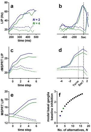
for*_{40 ms in LIP, then “fork”: they continue ramping-up if dots moved towards the response} (or movement) field of the neuron (inRF trials;Fig 6a, solid lines) or drop their slope if the dots were moving away from its response field (outRF trials; dashed lines) [1,3]. Striatal neu-rons exhibit an analogousramp-and-forkpattern of response (Fig 7c and 7d). The magnitude of LIP firing rate is inversely proportional to the number of available alternatives (Fig 6a and 6b) [3,46]; a phenomenon also recorded in other visuo-motor sites, notably in the superior colliculus [47] and FEF [48–50].

The model LIP (sensorimotor cortex) in rMSPRT captures each of these properties: activity ramps from the start of the accumulation, forks between putative in- and out-RF responses, and scales with the number of alternatives (Fig 6c). Under this model, inRF responses in LIP occur when the likelihood function represented by neurons was best matched by the uncertain MT evidence; correspondingly, outRF responses occur when the likelihood function was not well matched by the evidence.

The rMSPRT embodies a mechanistic explanation for the ramp-and-fork pattern in the two cases ofEq 9. Initial accumulation (steps 0–2 in our simulations; feedforward inference) occurs before the feedback has arrived at the model sensorimotor cortex, resulting in a ramp. The forking (step 3; start of feedback inference) is the point at which the posteriors from the output of the model basal ganglia first arrive at sensorimotor cortex to be re-used as priors. By con-trast, non-recursive MSPRT (without delayed feedback of posteriors) predicts well-separated neural signals throughout (Fig 6e). With recursion as the key difference, our framework sug-gests, first, that the ramp-and-fork pattern gives away the existence of an underpinning delayed inhibitory drive within a looped architecture—here from the model basal ganglia. Sec-ond, that the fork represents the time at which updated signals representing the competition between alternatives (posterior probabilities in the rMSPRT) are first made available to the sensorimotor cortex.

The rMSPRT further predicts that the scaling of activity in sensorimotor sites by the num-ber of alternatives is due to cortico-subcortical loops becoming transiently organized asN par-allel functional circuits, one per hypothesis. This would determine the baseline output of the basal ganglia. Until task related signals reach the model basal ganglia output, it codes the initial priors for the set ofNhypotheses. Their output is then an increasing function of the number of alternatives (Fig 6f). This increased inhibition of thalamus in turn reduces baseline cortical activity as a function ofN. The inverse proportionality of cortical activity toNin macaques during decisions (Fig 6a and 6b; [3,46,48,49]) and the direct proportionality of the firing rate toNin their SNr [42] lend support to this hypothesis.

The rMSPRT also captures key features of dynamics at decision termination. For inRF tri-als, the mean firing rate of LIP neurons peaks at or very close to the time of saccade onset (Fig 6b). By contrast, for outRF trials mean rates appear to fall just before saccade onset. The rMSPRT can capture both these features (Fig 6d) when we allow the algorithm to continue updating after the decision rule (Eq 10) is met. The decision rule is implemented at the output of the basal ganglia and the model sensorimotor cortex peaks just before the final posteriors have reached it. The rMSPRT thus predicts that the activity in LIP lags the actual decision.

Fig 6. Example LIP firing rate patterns and predictions of rMSPRT and MSPRTat 25.6% coherence.(a, b) Mean population firing rate of LIP neurons during correct trials on the reaction-time version of the dot motion task (19 neurons). By convention, inRF trials are those when recorded neurons had the motion-cued target inside their response field (solid lines); outRF trials are those when that target was outside the neuron’s response field (dashed lines). (a) Aligned at stimulus onset, starting at the stereotypical dip, illustrating the “ramp-and-fork” pattern between average inRF and outRF responses. (b) Aligned at saccade onset (vertical dashed line). (c, d) Mean time course of the model sensorimotor cortex in rMSPRT aligned at decision initiation (c;t= 1) and termination (d; Term; dotted line), for correct trials. Initiation and termination are with respect to the time of basal ganglia output. Note the suggested saccade time “Sac?”, close to the peak of inRF computations. Simulations are a single Monte Carlo experiment with 800, 1200 total trials forN= 2, 4, respectively, using parameter setO_{d. For simplicity the (r)MSPRT is simulated in} discrete time steps, but these have an interpretation in continous time (seeMethods). We include an additional step at

−1 determined only by initial priors and baseline, where no inference is carried out (yi(t+ yb) = 0 for alli; see Methods). Conventions as in (a). (e) Same as in (c), but for the standard, non-recursive MSPRT (Eq 10using only the first case of Eqs8and9). (f) Baseline output of the model basal ganglia increases as a function of the number of alternatives, thus increasing the initial inhibition of thalamus and cortex. For uniform priors, the rMSPRT predicts this function is:−logP(Hi) =−log (1/N). Coloured dots indicateN= 2 (blue) andN= 4 (green).

In the rMSPRT, the striatum relays the input from sensorimotor cortex as an inhibitory drive for downstream basal ganglia nuclei. The rMSPRT has three free parameters that shape the ramp-and-fork of its inner variables, but do not alter inference. We have set their value to show that mapped variables can match the pattern in sensorimotor cortical neural dynamics (seeMethods); below we show how these predictions depend on the parameter values.

Fig 7. Modulation of activity by coherence throughout the cortico-basal-ganglia-thalamo-cortical loops.(a-j) N= 2. (k-r)N= 4. Top row: mean population firing rate in LIP over time during the random dot motion task (19 neurons), aligned to stimulus onset (Stim; a, k) or saccade onset (Sac; b, l) (vertical dashed lines). (c, d) mean population firing rate in striatum during the dots task (48 neurons); same conventions as in top row. (e-j, m-r) mean rMSPRT computations as mapped inFig 5, aligned at decision initiation or termination (Init/Term; dotted lines); single Monte Carlo experiment with 800, 1200 total trials forN= 2, 4, respectively; simulation as inFig 6c–6e. (e, f, m, n) predicted time course of the model sensorimotor cortex (e.g.LIP) or striatum. (g, h, o, p) predicted simultaneous course of mean firing rate in SNr. (i, j, q, r) predicted course in thalamic relay nuclei. Solid: inRF. Dashed: outRF. Coherence % as in legend. Unshaded regions indicate approximate periods where a mechanism of decision formation should aim to reproduce the recordings.

Nonetheless, the rMSPRT with these parameters also captures the ramp-and-fork pattern of activity in the monkey striatum (compare panels c, d to e, f inFig 7).

LIP and striatal firing rates are also modulated by dot-motion coherence (Fig 7a–7d, 7k, 7l). Following stimulus onset, the response of these neurons tends to fork more widely for higher coherence levels (Fig 7a, 7c and 7k) [1,3,6]. The increase in activity before a saccade during inRF trials is steeper for higher coherence levels, reflecting the shorter average reac-tion times (Fig 7b, 7d and 7l) [1,3,6]. The sensorimotor cortex or striatum in the rMSPRT shows coherence modulation of both the forking pattern (Fig 7e and 7m) and slope of activity increase (Fig 7f and 7n). rMSPRT also predicts that the apparent convergence of peri-sac-cadic LIP activity to a common level during inRF trials (Fig 7b and 7l) is not required for inference and so may arise due to additional neural constraints. We take up this point in the Discussion.

Electrophysiological predictions

Our proposed mapping of the rMSPRT’s components (Fig 5) makes testable qualitative predic-tions for the mean responses in basal ganglia and thalamus during the dot motion task. For the basal ganglia output, likely from the oculomotor regions of the SNr, rMSPRT (like MSPRT) predicts a drop in the activity of output neurons during inRF trials and an increase in outRF ones. It also predicts that these changes are more pronounced for higher coherence levels (Fig 7g, 7h, 7o and 7p). These predictions are consistent with recordings from macaque SNr neu-rons showing that they suppress their inhibitory activity during visually- or memory-guided saccade tasks, in putative support of saccades towards a preferred region of the visual field [42,

51,52], and enhance it otherwise [52].

In detection tasks like visually- or memory-guided ones, the decision cues are extremely obvious. Hence, the accompanying recorded neural-activity transients may be argued to encode very short evidence-accumulations. After all, the accumulation of a single observation (e.g.an ISI) is the simplest, albeit degenerate case of evidence accumulation.

For visuo-motor thalamus, rMSPRT predicts that the time course of the mean firing rate will exhibit a ramp-and-fork pattern similar to that in LIP (Fig 7i, 7j, 7q and 7r). The separa-tion of in- and out-RF activity is consistent with the results of [33] who found that, during a memory-guided saccade task, neurons in the macaque medio-dorsal nucleus of the thalamus (interconnected with LIP and FEF), responded more vigorously when the saccade target was flashed within their response field than when it was flashed in the opposite location.

Predictions for neural activity features not crucial for inference

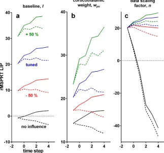
Understanding how a neural system implements an algorithm is complicated by the need to identify which features are core to executing the algorithm, and which are imposed by the con-straints of implementing computations using neural elements—for example, that neurons can-not have negative firing rates, so cancan-not straightforwardly represent negative numbers. The three free parameters in the rMSPRT allow us to propose which functional and anatomical properties of the cortico-basal-ganglia-thalamo-cortical loop are workarounds within these constraints, but do not affect inference.

The second free parameter,wyt, sets the strength of the spatially diffuse projection from

cor-tex to thalamus. Varying this weight changes the forking between inRF and outRF computations but does not affect inference (Fig 8b). The third free parameter,n, sets the overall, hypothesis-independent temporal scale at which sampled input ISIs are processed; changingnvaries the slope of sensorimotor computations, even allowing all-decreasing mean firing rates (Fig 8c). By definition, the log-likelihood of a sequence tends to be negative and decreases monotonically as the sequence lengthens. Introducingnis required to get positive simplified log-likelihoods, capable of matching the neural activity dynamics, without affecting inference. Hence,nmay capture a workaround of the decision-making circuitry to represent these whilst avoiding signal ‘underflow’, by means of scaling the input data.

Traditionally, evidence accumulation is exclusively associated with increasing firing rates during decision, and previous studies have questioned whether the often-observed decision-correlated yet non-increasing firing rates (e.g.in outRF conditions inFig 7a, 7c and 7kand [1–

3,5,53,54]) are consistent with accumulation [22,23]. The diversity of patterns predicted by rMSPRT in sensorimotor cortex (Fig 8) solves this by demonstrating that both increasing and non-increasing activity patterns can house evidence accumulation.

Fig 8. Effect of variations of free parameters on the time course of the model LIPin rMSPRT.Each solid and dashed set of lines is the mean of correct trials in a single Monte Carlo experiment, with 800 total trials, 25.6% coherence andN= 2; simulation as inFig 6c–6e. Computations aligned at decision initiation. Solid: inRF. Dashed: outRF. Blue: with parameters as tuned for this study. Green: increasing parameter value by 50%, keeping other parameters as tuned. Red: decreasing it by 50%, keeping others as tuned. Black: removing the effect of the tested parameter (l= 0,wyu= 0,n= 1), keeping others as tuned. (a) Varying the baseline,l. (b) Varying the cortico-thalamic weight,wyu. (c) Varying the data scaling factor,n.

Discussion

We tested the hypothesis that the brain approximates exact inference for decision making. We did so by showing that a novel recursive form of the MSPRT, the rMSPRT, uniquely accounts for both monkey choice behaviour and the corresponding neural dynamics in cortex and stria-tum, while its architecture matches that of the cortico-subcortical decision circuits.

Why implement a recursive procedure in the brain?

The recursive computation implied by the looped cortico-basal-ganglia-thalamo-cortical architecture has several advantages over local or feedforward computations. First, recursion makes trial-to-trial adaptation of decisions possible. Priors determined by previous stimulation (fed-back posteriors), can bias upcoming similar decisions towards the expected best choice, even before any new evidence is collected. This can shorten reaction times in future familiar settings without compromising accuracy. Second, recursion provides a robust memory. A pos-terior fed-back as a prior is a sufficient statistic of all past evidence observations. That is, it has taken ‘on-board’ all sensory information since the decision onset. In rMSPRT, the sensorimo-tor cortex only need keep track of observations in a moving time window of maximum width Δ—the delay around the cortico-subcortical loop— rather than keeping track of the entire sequence of observations. For a physical substrate subject to dynamics and leakage, like a neu-ron in LIP or FEF, this has obvious advantages: it would reduce the demand for keeping a per-fect record (e.g.likelihood) of all evidence, from the usual hundreds of milliseconds in decision times to the*_{30 ms of latency around the cortico-basal-ganglia-thalamo-cortical} loop (adding up estimates from [55–57]).

Lost information and perfect integration

The rMSPRT decides faster than monkeys in the same conditions because monkeys do not make full use of the discrimination information available in their MT (Fig 3b). However, this performance gap arises partially because rMSPRT is a generative model of the task. Thus, this assumes that knowledge of coherence is available by decision initiation, which in turn deter-mines appropriate likelihoods for the task at hand. Any deviation from this generative model will tend to degrade performance, whether it comes from one or more of: the coherence to likelihood mapping [58], the inherent leakiness of neurons, or correlations between spikes or between neurons (see [20]). In this respect, we must consider, first, that the activity dip*₁₇₀ ms after stimulus onset is assumed to indicate decision engagement at the LIP level. By then, MT neurons have been reliably modulated by motion coherence for about 120 ms (start-ing*_{50 ms after stimulus onset; seeS4 Figfor details), giving a sizeable window to adjust LIP} ‘likelihood functions’ to match the decision at hand. Whether this window is large enough or if trial-by-trial ‘likelihood adjustment’ occurs at all remain as interesting questions for future experimental explorations. Second, that LIP neurons change their coding during learning of the dot motion task and MT neurons do not [59], implying that learning the task requires mapping of MT to LIP populations by synaptic plasticity [60]. Consequently, even if the MT representation is perfect, the learnt mapping only need satisfice the task requirements, not optimally perform.

task, and further support the idea that the neural decision-making mechanism can perform perfect integration of uncertain evidence.

Neural response patterns during decision formation

Neurons in LIP, FEF [4], and striatum exhibit a ramp-and-fork pattern during the dot motion task. Analogous choice-modulated patterns have been recorded in the medial premotor cortex of the macaque during a vibro-tactile discrimination task [53] and in the posterior parietal cor-tex and frontal orienting fields of the rat during an auditory discrimination task [5]. The rMSPRT indicates that such slow dynamics emerge from decision circuits with a delayed, inhibitory drive within a looped architecture. This suggests that decision formation in mam-mals may use a common recursive computation.

A random dot stimulus pulse delivered earlier in a trial has a bigger impact on LIP firing rate than a later one [2]. This highlights the importance of capturing the initial, early-evidence ramping-up before the forking. However, multiple models omit it, focusing only on the fork-ing (e.g.[9,10,13]). Other, heuristic models account for LIP activity from the onset of the choice targets, through dots stimulation and up until saccade onset (e.g.[12,14–16]). Never-theless, their predicted firing rates rely on two fitted heuristic signals that shape both the post-stimulus dip and the ramp-and-fork pattern. In contrast, the ramp-and-fork dynamics emerge naturally from the delayed inhibitory feedback in rMSPRT during decision formation.

rMSPRT qualitatively replicates the ramp-and-fork pattern for individual coherence levels and given number of alternatives,N(Fig 6). However, the peak of the accumulated evidence in the model sensorimotor cortex of rMSPRT does not converge to a common value around deci-sion termination during inRF trials. Consequently, it predicts that the apparent convergence of LIP activity to a common value (Figs6band7b and 7l) is not part of the inference proce-dure, but reflects other constraints on neural activity.

One such constraint is that these brain regions engage in multiple other computations, some of which are likely orthogonal to solving the random dot motion task. The neural activity recorded during decision tasks may then be a transformation of inference computations, by mixing them with all other simultaneous computations. Consistent with this, the successful fit-ting of previous computational models to neural data [12,14–16] has been critically dependent on the addition of heuristic signals for unknown constraints. While beyond the scope of this study, which examined whether a normative mechanism could explain behaviour and electro-physiology during decisions, adding similar heuristic signals to the rMSPRT would likely allow a quantitative reproduction of the peri-saccadic convergence of LIP activity.

Emergent predictions

the firing rate in SNr and thalamic nuclei naturally emerge from the functional mapping of the algorithm onto the cortico-basal-ganglia-thalamo-cortical circuitry. These are already congru-ent with existing electrophysiological data; however, their full verification awaits recordings from these sites during the dot motion task. These and other emergent predictions are an encouraging indicator of the explanatory power of a systematic framework for understanding decision formation, embodied by the rMSPRT.

Relation of the rMSPRT to prior decision models

The rMSPRT contains all previous instances of the MSPRT [17,18,25,26,62] as special cases. It generalizes them by allowing the re-use of posteriors at any given time in the past as priors for present inference, via recursion. The (r)MSPRT also contains the sequential probability ratio test whenN= 2, and its continuous-time equivalent, the popular drift-diffusion model (e.g.[4,6,9,61,63–66]). While a valuable basic model of decision-making, the drift-diffusion model is restricted toN= 2 alternatives and does not address neural mechanisms. First, it assumes that evidence for decisions comes as a continuous Gaussian process whose presence in the brain is unproven. Since the decision times predicted by the model critically hinge on this process and its statistics (typically disconnected from the statistics of sensory neural activ-ity), this limitation also obscures the interpretation of the drift-diffusion model’s behavioural predictions. Second, its single decision variable must restrict itself to the half-plane closest to the choice threshold associated to one of its two hypotheses if such hypothesis is to be chosen; hence, the drift-diffusion model can account for forking dynamics, but not for the preceding ramping observed in experimental data. In contrast, the rMSPRT natively captures decisions among any number of alternatives (N2), can explain ramp-and-fork dynamics, and does so using neural evidence for decisions in its natural format: spike-trains with statistics extracted from MT recordings.

Biophysical models that directly address neural implementations of decision making are predominantly based on winner-take-all competition between neurons representing different hypotheses [8,11–14,16,67,68]. These provide valuable insights into potential mechanisms by which neural circuits can represent and compute decisions, but do not typically make con-tact with formal inference procedures (see [69]). The studies of [13,68] are possible exceptions, since they make the analogy between the predictions of their neural-network model and those of exact, Bayes-based inference. Conversely, the rMSPRT shows how a normative decision-making algorithm can account for cortical and subcortical activity. As such, the rMSPRT pro-vides target, exact-inference computations for future biophysical models.

Anatomical mapping, assumptions, and future directions

Mapping any formal algorithm to a neural substrate implies proposing assumed computa-tional contributions for the components of the substrate. In mapping the rMSPRT we made two broad classes of assumptions. First, as explained above, that individual substrates imple-ment multiple functions either simultaneously or under different stimulation scenarios (e.g.

avenue for future research is determining if, and how, the dynamics of the striatal micro-cir-cuit can act as a relay-like function during decision formation.

Our second class of assumptions is that the omitted connections into and within the basal ganglia may not contribute to the computations essential to inference with cortical inputs. Of note, we have omitted in our mapping the projections from thalamus to striatum [76] or to subthalamic nucleus [77], as well as the intrinsic connections from subthalamic nucleus or from globus pallidus pars externa (globus pallidus in non-primates) to striatum (e.g.see [77,

78]). Such omitted connections might offer a more robust implementation of inference com-putations, or may contribute to overcoming the limitations of implementing an algorithm with neurons.

Demonstrating the compatibility of anatomical pathways with the mapping of the (r)MSPRT is the subject of ongoing research. Success has been achieved in the expansion of the basal-ganglia mapping of the MSPRT to include the pathway from striatum to globus palli-dus pars externa and that from the latter to SNr, where the same inference could be done with-out those pathways [17]. It has also been recently shown that the pallido-striatal connection is compatible with the MSPRT mapping onto the basal ganglia [21], possibly giving a more robust neural implementation. Both results carry to the rMSPRT. In the same bracket is our inclusion of the cortico-thalamic projection here (Fig 5). Since this projection is assumed to be hypothesis-independent (Eq 12), it does not affect the inference done by the rMSPRT. Similar exercises may be able to account for projections from thalamus to striatum or to subthalamic nucleus, and from the latter to striatum, though these are beyond the scope of this study. The rMSPRT provides a starting point to explore all such extended mapping alternatives.

Conclusion

We sought to characterize the neural mechanism that underlies decisions using a normative algorithm—the rMSPRT—as a framework. We find it remarkable that, starting from data-con-strained spike-trains, our monolithic statistical test can simultaneously account for much of the anatomy, behaviour, and electrophysiology of decision-making. While it is not plausible that the brain implements exactly a specific algorithm, our results suggest that the essential composition of its underlying decision mechanism includes the following. First, that the mech-anism is probabilistic in nature—the brain utilizes the uncertainty in neural signals, rather than suffering from it. Second, that the mechanism works entirely ‘on-line’, continuously updating representations of hypotheses that can be queried at any time to make a decision. Third, that this processing is distributed, recursive, and parallel, producing a decision variable for each available hypothesis. And fourth, that this recursion allows the mechanism to adapt to the observed statistics of the environment in an unsupervised manner, as it can re-use updated probabilities about hypotheses as priors for upcoming decisions. With the currently available range of experimental studies giving us local snapshots of cortical and subcortical activity dur-ing decision-makdur-ing tasks, the rMSPRT shows us how, where, and when these snapshots fit into a complete inference procedure.

Materials and methods

Experimental paradigms

Behavioural and neural data was collected in three previous studies [3,6,24], during two ver-sions of the random dot motion task (Fig 1a–1c). Detailed experimental protocols can be found in each report. Below we briefly summarize them.

covering the response field of the MT neuron being recorded (grey patch); task difficulty was controlled per trial by the proportion of dots (coherence %) that moved in one of two direc-tions: that to which the MT neuron was tuned to—its preferred motion direction—or its oppo-site—null motion direction. After 2 s the fixation point and kinematogram vanished and two targets appeared in the possible motion directions. Monkeys received a liquid reward if they then saccaded to the target towards which the dots in the stimulus were predominantly moving [24].

Reaction time. Two macaques per study learned to fixate their gaze on a central fixation point (Fig 1b and 1c). Two (Fig 1b) or four (Fig 1c; only in the protocol of [3]) eccentric targets appeared, signalling the number of alternatives in the trial,N. One such target fell within the response (movement) field of the recorded neuron (grey patch). This is the region of the visual field towards which the neuron would best support a saccade. Later a random dot kinemato-gram appeared where a controlled proportion of dots moved towards one of the targets. The monkeys received a liquid reward for saccading to the indicated target when ready [3,6].

Data analysis

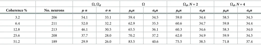
For comparability across databases, we only analysed data from trials with coherence levels of 3.2, 6.4, 12.8, 25.6, and 51.2%, unless otherwise stated. We used data from all neurons recorded in such trials. Our datasets contained between 189 and 213 visual-motion-sensitive MT neu-rons (seeTable 1; single-cell recordings from [24,79]), as well as 19 LIP neurons (data from [3]) and 48 striatal ones (from [6]) whose activity was previously determined to be choice- and coherence-modulated. The behavioural data analysed was that associated to LIP recordings. For MT, we analysed the neural activity between the onset and the vanishing of the stimulus. For LIP and striatum we focused on the period between 100 ms before stimulus onset and 100 ms after saccade onset.

To estimate moving statistics of neural activity we first computed the spike count over a 20 ms window sliding every 1 ms, per trial. The moving mean firing rate per neuron per condi-tion was then the mean spike count over the valid bins of all trials divided by the width of this window; the standard deviation was estimated analogously. LIP and striatal recordings were either aligned at the onset of the stimulus or of the saccade; after or before these (respectively), data was only valid for a period equal to the reaction time per trial. The population moving mean firing rate is the mean of single-neuron moving means over valid bins; analogously, the population moving variance of the firing rate is the mean of single neuron moving variances. For clarity, population statistics were then smoothed by convolving them with a Gaussian

Table 1. Population ISI statistics (ms) in MT per coherence (first column).

O,O_d O O_d,N= 2 O_d,N= 4

Coherence % No. neurons μn σn μ₀n σ₀n μ₀n σ₀n μ₀n σ₀n

3.2 206 54.1 33.1 59.4 34.5 59.0 34.4 58.5 34.3

6.4 211 52.0 32.2 62.9 35.3 60.6 34.7 59.8 34.4

12.8 213 46.1 30.5 65.5 36.1 60.3 34.6 58.3 34.0

25.6 208 37.7 28.0 70.2 37.2 62.0 34.9 59.9 34.3

51.2 189 29.9 26.0 83.5 40.6 75.5 38.5 71.8 37.4

Second column: number of neurons for which data was available per coherence.μ: mean.σ: standard deviation.n: data scaling factor. Statistics with subscriptdenote

that dots were moving towards the preferred motion direction of the MT neuron, whereas0denotes that they were moving in the opposite, null direction. The

parameter set,O_{(computed here from MT data) or}O_{d(after information depletion), to which each value corresponds is noted above them. Note that, due to the} information depletion required to produceO_d,μ0nandσ0ntake different values forN= 2, 4.

kernel with a 10 ms standard deviation. The resulting smoothed population moving statistics for MT are inFig 1d and 1e. LIP and striatal mean firing rates are plotted only up to the median reaction time plus 80 ms, per condition.

Analogous procedures were used to compute the moving mean of the computations within simulated algorithms, per time step, rather than over a moving window. These are shown up to the median of termination observations plus 3 time steps.

Definition of the recursive multi-hypothesis sequential probability ratio

test (rMSPRT)

Letx(t) = (x1(t),. . .,xC(t)) be a vector random variable composed of scalar observations, xj(t), made inCchannels at timet2{1, 2,. . .} (right-hand side ofFig 9). Let alsox(r:t) =

(x(r)/n,. . ._{,x(t)/n) be the sequence of vectorsx(t)/n, i.i.d. across time, fromrtot(r<t). Here}

n2 fR>0_{gis a constant data scaling factor. Ifn>1, it scales down incoming data,xj(t); this} will prove useful ahead when tuning the algorithm to reveal that the dynamics in rMSPRT computations match those of sensorimotor cortex. Note that scaling is only effective from the likelihood on and does not affect the time interpretation of the data. Crucially, sincenis hypothesis-independent, it does not affect inference.

There areN2{2, 3,. . ._{} alternatives or hypotheses about the uncertainevidence,x(1:t)—} say possible courses of action or perceptual interpretations of sensory data. The task of a deci-sion maker is to determine which hypothesisHi(i2{1,. . .,N}) is best supported by this

evi-dence as soon as possible, for a given level of accuracy. To do this, it requires to estimate the posterior probability of each hypothesis given the data,P(Hi|x(1:t)), as formalized by Bayes’

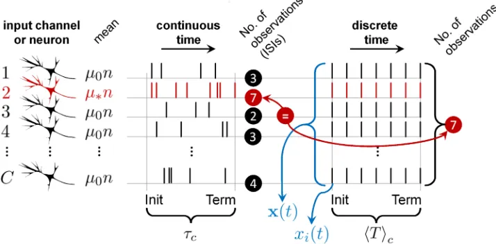
Fig 9. The mean number of ISIs to decision in continuous-time spike-trains is equivalent to the mean number observations to decision in discrete time.Csensory neurons (input channels; left) produce sequences of ISIs in continuous time with meanμn(red; best tuned to the stimulus) orμ₀n(black; otherwise). The average decision time—

between decision initiation (Init) and termination (Term)—isτcin correct trials, as in this diagram. In discrete time it takes an average ofhTicvector observations,x(t) (composed of scalar observationsxi(t), each time stept; blue), to make decisions. [20] showed that in the minimum input case (whenC=N), the mean number of ISIs in the most active channel (red) used by a general, continuous-time, spike-based instance of the MSPRT, approximately equal the mean number of observations,hTic, required by the simpler, discrete-time MSPRT (here 7 in both cases), which carries to our identically-performing rMSPRT; this is true under equal input channel statistics (μ,μ₀,σ,σ₀), data distributions

(e.g.all lognormal), number of alternatives,N, and error rate,. This all implies that, if we add 0.5—the expected number of ISIs from decision initiation to a first spike—tohTic, and multiply this by the minimum mean ISI,μn(of

fastest firing channel), this approximately equalsτc, henceEq 14; conversely, in error trials we useμ0andhTie, to getτe

(Eq 15).

rule. The mechanism we seek must be recursive to match the nature of the brain circuitry. For-mally,P(Hi|x(1:t)) will be initially computed upon starting priorsP(Hi) and likelihoodsP(x(1: t)|Hi); however, after some timeΔ2{1, 2,. . .}, it will re-use past posteriors,P(Hi|x(1:t−Δ)),Δ

time steps ago, as priors, along with the likelihood functionP(x(t−Δ+ 1:t)|Hi) of the segment

ofx(1:t) not yet accounted byP(Hi|x(1:t−Δ)). A mathematical induction proof of this form

of Bayes’ rule follows.

If sayΔ= 2, in the first time step,t= 1:

P Hð ijxð1Þ=nÞ ¼

Pðxð1_{Þ=njHiÞPðHiÞ}

Pðxð1_Þ=nÞ ð1Þ

Byt= 2:

P Hð ijxð2Þ=n;xð1Þ=nÞ ¼

Pðxð2_Þ=n;xð1_Þ=njH

iÞPðHiÞ Pðxð2_Þ=n;xð1_Þ=nÞ

Note that we are still using the initial fixed priorsP(Hi). Now, fort= 3:

P Hð ijxð3Þ=n;xð2Þ=n;xð1Þ=nÞ ¼

Pðxð3_Þ=n;xð2_Þ=n;xð1_Þ=njH

iÞPðHiÞ

Pðxð3_Þ=n;xð2_Þ=n;xð1_Þ=nÞ ð2Þ

According to the product rule, we can segment the probability of the sequencex(1:t) as:

Pðxð1 :tÞÞ ¼Pðxðt Dþ1 :tÞ;xð1 :t DÞÞ ¼

Pðxðt Dþ1 :tÞjxð1 :t DÞÞPðxð1 :t DÞÞ ð

3Þ

And, sincex(t) are i.i.d., the likelihood of the two segments is:

Pðxð1 :_{tÞjHiÞ ¼Pðxðt} D_þ1 :_{tÞjHiÞPðxð}1 :_t D_ÞjH

iÞ ð4Þ

If we substitute the likelihood inEq 2byEq 4, its normalization constant byEq 3and re-group, we get:

P Hð ijxð3Þ=n;xð2Þ=n;xð1Þ=nÞ ¼

Pðxð3_Þ=n;xð2_Þ=njHiÞ

Pðxð3_Þ=n;xð2_Þ=njxð1_Þ=nÞ

Pðxð1_{Þ=njHiÞPðHiÞ}

Pðxð1_Þ=nÞ

It is evident that the rightmost factor isP(Hi|x(1)/n) as inEq 1. Hence, in this example, by t= 3 we start using past posteriors as priors for present inference as:

P Hð ijxð3Þ=n;xð2Þ=n;xð1Þ=nÞ ¼

Pðxð3_Þ=n;xð2_{Þ=njHiÞPðHijxð}1_Þ=nÞ

Pðxð3_Þ=n;xð2_Þ=njxð1_Þ=nÞ

So, in general:

PðHijxð1 :tÞÞ ¼

Pðxð1 :_{tÞjHiÞPðHiÞ}

Pðxð1 :_tÞÞ for tD

Pðxðt D_þ1 :_tÞjH

iÞPðHijxð1 :t DÞÞ

Pðxðt D_þ1 :_tÞjxð1 :_t D_ÞÞ for t>D 8

> > > <

> > > :

where the normalization constants are

Pðxð1 :_{tÞÞ ¼}PN

j¼1Pðxð1 :tÞjHjÞPðHjÞ

Pðxðt D_þ1 :_tÞjxð1 :_t D_{ÞÞ ¼}PN

j¼1Pðxðt Dþ1 :tÞjHjÞPðHjjxð1 :t DÞÞ

Eq 5is a general recursive form of the Bayes’ rule, designed to accumulate evidence for inference in a recurrent, uninterrupted fashion. Byt>Δ, it uses posteriorsΔ1 time steps in the past as current priors, thereby generalizing a previous common recursive form of the Bayes’ rule that is limited toΔ= 1 (that ine.g.[18,26,68,80,81]). Priors updated in this man-ner are a sufficient statistic of all the evidence observed up tot−Δ. By this ability, and in the

general machine-learning sense, any decision algorithm harnessingEq 5adapts or learns. Since no labelled examples or teaching signals are required for such learning, the rMSPRT is thence said to be engaged in ongoingunsupervised learning.

Ahead we use three key results from [20] as part of our methods, with no overlap between their results and the results of the present study. First, a lognormal-based form of the likeli-hood function whose component operations they showed are neurally plausible and most con-sistent with the statistics of MT responses during the random dots task. Second, a crucial link between the statistics of ISIs in the spike-trains used as evidence for decision (e.g.those of MT during the dots task), and continuously-distributed MSPRT decision times. As discussed below, this link enabled us to use simpler, discrete-time algorithms and still interpret their behavioural predictions in continuous time. And third, the fundamental dependence of MSPRT decision times on: (a) the discrimination information available in the evidence and (b) a constant, fixed for given error rate andN. Since rMSPRT performs identically to MSPRT, all this carries to it.

It is apparent that the critical computations inEq 5are the likelihood functions. The forms that we consider ahead build upon the simplest shown by [20], where the number of evidence streams equals the number of hypotheses (C=N); for instance, a minimum ofC= 2 differ-ently-tuned neurons are assumed to provide evidence for aN= 2 choice decision. As discussed by them, more complex (C>N), biologically-plausible likelihood functions can be formulated if necessary; theC<Ncase would make no sense as it would imply the testing of redundant hypotheses. Although not essential, to simplify the notation whenC=N, from now on data in the channel conveying the most salient evidence for hypothesisHiwill bear its same indexi, as xi(j). WhentΔwe have:

Pðxð1 :_{tÞjHiÞ ¼aðtÞ}Y

t

j¼1

fðxiðjÞ=nÞ

f0ðx_iðjÞ=nÞ ð

6Þ

this is, the likelihood thatxi(j)/nwas drawn from a distribution,f, rather than fromf₀,

that is assumed to have originatedxk(j)/n(k6¼i) for the rest of the channels. InEq 6, aðtÞ ¼Qt

m¼1 QN

k¼1f0ðxkðmÞ=nÞis a hypothesis-independent factor that does not affectEq 5

and thus needs not to be considered further.

Whent>Δonly the observations in the time window [t−Δ+ 1,t] are used for the likeli-hood function because data before this window is already considered within the fed-back pos-terior,P(Hi|x(1:t−Δ)). Then, the likelihood function is:

Pðxðt D_þ1 :_{tÞjHiÞ ¼dðtÞ} Y

t

j¼t D_þ1

fðxiðjÞ=nÞ

f0ðx_iðjÞ=nÞ ð

7Þ

where againdðtÞ ¼Qt

m¼t D_þ1 QN

Now, for our likelihood functions to work upon a statistical structure like that produced by neurons in MT we need to be more specific. Inter-spike intervals (ISI) in MT during the ran-dom dot motion task are best described as lognormally distributed [20] and we assume that decisions are made upon the information conveyed by them. Thus, from now on we assume thatfandf₀are lognormal and that they are specified by meansμandμ₀, and standard devia-tionsσandσ₀, respectively. We can then put together the logarithm of Eqs6and7as the log-likelihood function,yi(t), substituting the lognormal-based form of it reported by [20]:

yiðtÞ ¼

g0Dþg1 Pt

j¼1½logðxiðjÞ=nފ 2

þg2 Pt

j¼1logðxiðjÞ=nÞ for tD g0Dþg1

Pt

j¼t D_þ1½logðxiðjÞ=nފ 2

þg2 Pt

j¼t D_þ1logðxiðjÞ=nÞ for t>D

8 <

:

ð8Þ

with

g0 ¼ k2

0 2Y2

0 k2

2Y2

þlog Y0

Y

g1 ¼ 1

2Y2₀ 1

2Y2

g2¼ k

Y2

k0

Y2₀

wherek¼ logðm2

= ffiffiffiffiffiffiffiffiffiffiffiffiffiffiffi

s2 þm2 p

ÞandΘ2_{= log(}

σ2/μ2+ 1) with appropriate subindices,₀.

The termsg0ΔinEq 8are hypothesis-independent, can be absorbed intoa(t) andd(t),

cor-respondingly, and thus will not be considered further. As a result of this, theyi(t) used from

now on is a “simplified” version of the log-likelihood.

We now take the logarithm ofEq 5, define−logPi(t)−logP(Hi|x(1:t)) and substitute the

simplified log-likelihood fromEq 8in the result, giving:

logPiðtÞ ¼

ziðtÞ logPðHiÞ þlog

XN

j¼1

expðzjðtÞ þlogPðHjÞÞ for tD

ziðtÞ logPiðt DÞ þlog

XN

j¼1

expðzjðtÞ þlogPjðt DÞÞ for t>D

8 > > > > > < > > > > > :

ð9Þ

Wherezi(t) =yi(t) +c(t) and the termc(t) models a hypothesis-independent baseline. Because

of its uniformity across all hypotheses,c(t) has no effect on inference. It is defined in detail below.

The rMSPRT itself takes the form:

DðtÞ ¼

Choose hypothesisi: _{if logPiðtÞ ¼ min}

j2f1;...;Ng logPjðtÞ y;at t¼T

Continue sampling: _{if min}

j2f1_;..._;Ng logPjðtÞ>y; 8

<

:

ð10Þ