Carreau fluid in a wall driven corner flow

Contents lists available atScienceDirect

Journal of Non-Newtonian Fluid Mechanics

journal homepage:www.elsevier.com/locate/jnnfm

Carreau

fl

uid in a wall driven corner

fl

ow

S.T. Cha

ffi

n

⁎

, J.M. Rees

School of Mathematics and Statistics, University of Sheffield, Hicks Building, Hounsfield Road, Sheffield S3 7RH, UK

A R T I C L E I N F O

Keywords: Carreaufluid Wall driven cornerflow Matched asymptotic

A B S T R A C T

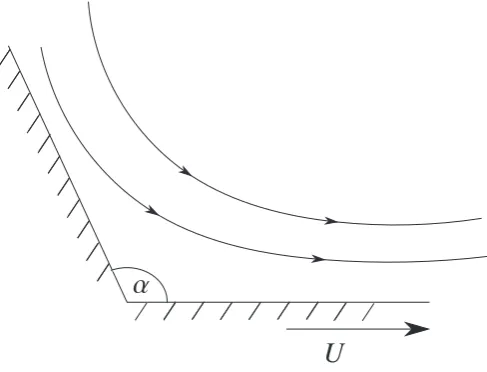
Taylor’s classical paint scraping problem provides a framework for analyzing wall-driven cornerflow induced by the movement of an oblique plane with afixed velocityU. A study of the dynamics of the inertialess limit of a Carreaufluid in such a system is presented. New perturbation results are obtained both close to, and far from, the corner. When the distance from the cornerris much larger thanUΓ, whereΓis the relaxation time, a loss of uniformity arises in the solution near the region, where the shear rate becomes zero due to the presence of the two walls. We derive a new boundary layer equation andfind two regions of widths_r−n_andr−2_{,whereris the} distance from the corner andnis the power-law index, where a change in behavior occurs. The shear rate is found to be proportional to the perpendicular distance from the line of zero shear. The point of zero shear moves in the layer of size_r−2_{. We alsofind that Carreau effects in the far-field are important for corner angles less than} 2.2 rad.

1. Introduction

Corner flows of both Newtonian and non-Newtonian fluids have been widely studied. Dean and Montagon[1]showed that for theflow of an inertialess Newtonianfluid, in plane polar coordinates (r,θ), the stream functionψ(r,θ) permits similarity solutions of the formrλf(θ). They identified the existence of a critical corner angle for whichλ be-comes complex. Later Moffatt[2]correctly asserted that these complex values would give rise to an infinite series of eddies of decreasing size. An experimental study by Taneda[3]revealed the existence of a series of decreasing eddies, thus confirming Moffatt’s theoretical predictions. Following Moffatt’s work, Proudman and Asadullah[4]considered the case of two inertialess immiscible Newtonian fluids of different viscosities with a planar contact line and found that the limit to a one phase system introduced an additional mode. Later, Henriksen and Hassager[5]studied power-lawfluids in a corner region, though due to physical constraints imposed on the power-law model, the results were limited to the parameter regime 0 <n< 2, wherenis the power-law exponent. Likewise, Keiller and Hinch[6]examined a system suspen-sion of rigid rods in a corner, but neglected the Brownian motion term of the constitutive equation in order to permit a similarity solution. They considered the aligned and unaligned orientations of the rods separately, but found that the solutions gave rise to unphysical eddies. In this study, we consider a two-dimensional incompressiblefluid that occupies the region between two semi-infinite planes (Fig. 1). One plane is moved with constant velocityUthat drives theflow. The other plane isfixed at an angleαrelative to the moving plane. In the vicinity

of the corner wall effects dominate, theflow and inertial terms become negligible so the creepingflow approximation can be used. This pro-blem wasfirst solved by Taylor[7]. Inertial effects were incorporated by Hancock et al. [8]by means of a perturbation expansion for the stream function. A study of the three-dimensional analogue of the paint scraping problem for a Newtonianfluid wasfirst presented by Hills and Moffatt [9], motivated by the fact that this mechanism is used throughout the chemical process industry to induce mixing. The un-derstanding of mixing in the chemical processing industry is of great importance as efficient mixing can improve consistency of products and reduce overall manufacturing costs[10,11]. As many industrialfluids exhibit non-Newtonian effects this motivates our further investigation into non-Newtonian fluids. The two-dimensional system has been analyzed for several types of non-Newtonian fluids. Riedler and Schneider[12]found an exact solution for a power-lawfluid in the creepingflow regime, and further considered the effects of leakage at the apex of the corner. Analysis of this geometry is not limited to power-lawfluids but can be applied to other constitutive relations[13]. The power-law model has the unphysical feature of having zero or infinite shear viscosity in regions where the shear rate tends to zero depending upon whethern is greater than or less than 1. Often an alternative model is needed to obtain correct physical behavior. The most com-monly used alternative is the Carreau model, where the kinematic viscosity,ν, is given by

= ∞+ − ∞ + − ν ν (ν0 ν )(1 Γ ˙ )2 2γ ,

n 1

2 ₍₁₎

whereγ˙ is the generalized shear rate,Γis the relaxation time andν∞

https://doi.org/10.1016/j.jnnfm.2018.01.002

Received 9 August 2017; Received in revised form 11 January 2018; Accepted 14 January 2018 ⁎_{Corresponding author.}

E-mail address:s.chaffin@sheffield.ac.uk(S.T. Chaffin).

0377-0257/ © 2018 The Authors. Published by Elsevier B.V. This is an open access article under the CC BY license (http://creativecommons.org/licenses/BY/4.0/).

andν0are the infinite shear and zero shear viscosities respectively. In the limit of low shear rates the viscosity approaches Newtonian beha-vior, thus overcoming the unphysical features of the power-law model. Throughout this article we will take ν∞=0, as this is a common as-sumption whenfitting experimental data to the Carreau model[14].

A Carreau fluid exhibits increased complexity in a wall-driven cornerflow in comparison to a power-lawfluid. This arises as it tran-sitions from exhibiting Newtonian behavior to power-law behavior in the geometry. The physics of this system does not permit a global self-similar solution, such as those that which can be found for the cases of purely Newtonian or purely power-law fluids. As no global solution exists, our approach will be to consider the solution in two different domains:firstly, in the region far from the corner apex, where the shear rates are low and the solution is approximately Newtonian with a small power-law correction, and secondly, in the vicinity of the corner apex, where the behavior is predominantly power-law coupled with a small Newtonian effect. It is worth noting that a global solution can be found for situations where the shear-rate has no radial dependence. This scenario occurs for the shear-driven problem and is discussed later in Section 7.

The structure of this article is as follows. The governing equations, boundary conditions and perturbation approach are discussed in Section 2.Section 3 presents the analysis of the system far from the corner, and the analysis near to the corner is described inSection 4. The matching process associated with the arising boundary layer system is analyzed in Section 5. The importance of eigen-modes and farfield conditions are discussed inSection 6. Conclusions and further discus-sion are given inSection 7.

2. Governing equations

The governing equations for the model are given by ∇ = −∇ + ∇τ

ρ( · )u u p · , (2)

∇·u=0, (3)

where τ is the viscous stress tensor given by τ=ρνγ˙ , where = ∇ + ∇

γ˙ u uT_{is the rate of deformation tensor,ρis the density andu} denotes the velocity field. The kinematic viscosity,ν, is given by(1) with the generalized shear rateγ˙2=1γ γ˙ : ˙

2 . Under the scalings

=U∼ r=U r p= ρνp τ= ρν

u u, Γ , τ

Γ , Γ ,

͠ 0͠ 0͠

(4) the system reduces to

∇ = ∇ + ∇ =

∼∼∼ ∼ ∼

Re( · )u u ·( )τ͠ p͠, τ͠ ν γ͠( ˙ ) ˙͠ γ͠ (5)

∇∼= ∼

u

· 0, (6)

where the scaled kinematic viscosity is given byν γ͠( ˙ )͠ =(1+γ˙ )͠2n−₂1

and the Reynolds number is given byRe=U2Γ/ν

0. Henceforth we assume

that the Reynolds number is sufficiently small that the inertial terms are negligible. Using the parameters fromTable 1and assuming that all of thefluids have density of approximately 103 kg m−3_{, we can obtain}

estimates forUfor which the inertial terms can be neglected. The most restrictive case (fluid A1) requires that for inertia to be negligible U≪0.1 m s−1_{. The least restrictive case (fluid A4) gives the condition}

U≪4 m s−1_{. Henceforth, we drop tilde notation for convenience.}

Mass conservation can be satisfied by the introduction of a stream-functionΩand the pressure can be eliminated by taking the curl of Eq. (5). Thus, the momentum equation can be expressed in terms of the stress tensorτ:

⎜ ⎟

⎛ ⎝

− ∂

∂ +

∂ ∂

∂

∂ +

∂

∂ ∂ −

⎞ ⎠ =

−

{

}

r r

τ

θ r r r r τ r r θ r τ τ

1 1

( ) 1 { ( )} 0,

rθ

rθ θθ rr

1 2

2

2 2

(7) where the components ofτare given in terms of the stream-function by

⎜ ⎟

= − = ∂

∂ ∂

∂ =

⎛ ⎝

∂

∂ −

∂ ∂

∂ ∂

⎞ ⎠

{ }

{ }

τ τ ν γ

r r θ τ ν γ r θ r r r r

2 ( ˙ ) 1 Ω , ( ˙ ) 1 Ω 1 Ω ,

rr θθ rθ ₂

2

2

(8)

⎜ ⎟ ⎜ ⎟

= ⎛ ⎝ ∂ ∂

∂ ∂

⎞ ⎠

+ ⎛ ⎝

∂

∂ −

∂ ∂

∂ ∂

⎞ ⎠

{ }

{ }

γ

r r θ r θ r r r r

˙2 4 1 Ω 1 Ω 1 Ω .

2

2 2

2

2

(9) Eq. (7)is subject to no-slip and moving wall boundary conditions on the fixed and moving planes, respectively,

= ∂

∂ = =

= ∂

∂ = =

r θ θ

θ θ α

Ω 0, 1 Ω 1, on 0,

Ω 0, Ω 0, on .

(10) From the form of the boundary condition(10), if a global similarity solution were to exist one would expectΩ=rf θ( ). The problem with such an ansatz is that the radial viscosity behavior_{ν γ( ˙ )}∼₍₁+_r−1₎n−₂1_,

and thus no similarity solution is permitted. We note that for largerthe Newtonian effects dominate and that for smallrshear-thinning effects dominate. At such scales the problem proves amenable to mathematical analysis. To distinguish between these regimes we will introduce a scaled radius_E−1_R=_{r,whereR=O(1),and a scaled stream function}

= −

ψ _E 1Ω,_{whereψ=O(1). This allows one to formally separate the} behavior in the far regimeE→0(seeSection 3) and the near regime

→ ∞

E (seeSection 4). It is helpful to express the momentum equation and boundary conditions in terms of the scaled variables:

∇ × ∇ ⎡· (1_⎣ +_E2 2γ˙ )n−₂1γ˙⎤_⎦=0,

(11)

= ∂

∂ = =

= ∂

∂ = =

ψ R

ψ

θ θ

ψ ψ

θ θ α

0, 1 1, on 0,

0, 0, on ,

[image:2.595.41.285.56.242.2]

(12) Fig. 1.Sketch of the driven cornerflow system.

Table 1

A collection of Carreau parameters for a range offluids. Fluids A1 and A2 are polystryrene solutions with mass fractions 0.45 and 0.3, respectively[14]. Fluids A3 and A4 are wood flour polypropylene mixtures[15], with woodflour volume fractions of 0 and0.28, re-spectively. The viscosityμ0is the dynamic viscosity which is related to the kinematic

viscosity byν0=μ ρ0/.

Fluid n Γ(s) μ0(Pa s)

A1 0.304 1.11 8.08

A2 0.305 0.03 135

A3 0.652 0.319 1.18 × 103

[image:2.595.306.557.114.175.2]

where the shear-rate and rate of strain tensor are now expressed in terms of ψandR. We will proceed byfirst analyzing the far corner region inSection 3.

3. The far corner approximationE≪1

We seek a solution in the form of a regular perturbation series

∼ + + + ⋯

ψ ψ₀ 2ψ ψ

1 4 2

E E (13)

in the limit asE→0. In this limit, the natural expansion of the viscosity is given by

+ ∼ + ⎛

⎝ −

⎞

⎠ + ⎛⎝ −

⎞ ⎠⎛⎝

− ⎞

⎠ +

−

γ n γ n n γ

[1 ˙ ] 1 1

2 ˙ 1 2

1 2

3

2 ˙ ( ).

2 2n 1 2 2 4 4 6

2

E E E O E

(14) Substituting the expansion for the viscosity into the momentumEq. (7) and imposing the boundary conditions(10)one can see that the zeroth order term reduces to the Newtonian system, which is given by the biharmonic equation. The solution is given[16]as

= − + +

ψ₀ R B( sin( )θ Cθcos( )θ Dθsin( )),θ (15) whereB, C, Dare constants given by

= −

− = − =

− −

B α

α α C

α

α α D

α α α

α α

sin ( ),

sin ( ) sin ( ),

sin( )cos( ) sin ( ) . 2

2 2

2

2 2 2 2

(16) Proceeding toO E( )the momentum equation can be written as ∇4ψ = ∇ × ∇κ ·( ˙ ˙ ),γ γ

1 0

2

0 (17)

whereκ1=n−₂1,γ˙0andγ˙0are the zeroth order terms of the shear rate

and rate of deformation tensor, given by

= − − = _{e e} +_{e e}

γ˙0 2R 2( sin( )C θ Dcos( )), ˙θ γ0 γ˙ (0 r θ θ r), where er, eθ are unit vectors in ther,θdirections.Eq. (17)can now be expressed as

∇ = ⎧

⎨ ⎩ ∂

∂ − − −

⎫ ⎬ ⎭ −

ψ κ R

θ C θ D θ C θ D θ

8 [( sin cos ) ] 3( sin cos ) .

4

1 1 5

2

2

3 3

(18) Forψ1to have consistent dimensions, we seek a solution in the form

= − ψ₁ R f θ1 ( )

1 . Thus(18)reduces to

+ ″ + = ⎧

⎨ ⎩ ∂

∂ −

− − ⎫

⎬ ⎭

f f f κ

θ C θ D θ

C θ D θ

10 9 8 [( sin cos ) ]

3( sin cos ) , iv

1 1 1 1

2

2

3

3

(19) subject to the boundary conditions f(0)= ′f (0)=f α( )= ′f α( )=0. Eq. (19)can be solved analytically forf1and leads to the expression

= + + + + +

+ +

−

ψ R A B θ θ C D θ θ E F θ θ G H θ θ

{( )cos(3 ) ( )sin 3 ( )cos

( )sin },

1 1 1 1 1 1 1 1

1 1

(20) where

= − = −

= + = +

B C CD κ D DC D κ

F C D C κ H D DC κ 1

2( 3 ) ,

1

2(3 ) ,

3

2( ) ,

3

2( ) .

1 3 2 1 1 2 3 1

1 3 2 1 1 3 2 1

(21) The constantsA1,C1,E1,G1are then derived from the boundary con-ditions. For simplicity, we give the result for the caseα=π/2,for which

= −

⎧ ⎨ ⎩

− −

+ − − −

− + + + − +

+ +

ψ κ

R π π π θ θ

π π π θ θ

π π θ θ π

π θ θ

( 4) (8 8(3 4) )cos(3 )

(2( 16) 4 ( 12) )sin(3 )

( 8 24( 4) )cos ( 2(3 16)

12( 4) )sin }. 1

1

2 3

3 2

4 2

3 2 4

2

(22)

Proceeding tofind the second order contribution leads to the partial differential equation

∇4ψ = ∇ × ∇·[κ γ˙ ˙γ +κ γ˙ ˙γ +κ γ˙ ˙ ],γ

2 1 120 1 02 1 2 04 0 (23)

whereκ2=(n−1)(n−3)/8,γ˙ ,1 andγ˙1are theO E( 2)terms of the shear

rate and rate of deformation tensor and can be expressed as

= ″ + ″ − = ⎛

⎝ ⎜

− ′ ″ −

″ − ′

⎞

⎠ ⎟

− −

γ R f f f f R f f f

f f f γ

˙ 2 ( )( 3 ), ˙ 4 3

3 4 ,

1

2 4

0 0 1 1 1 3

1 1 1

1 1 1 (24)

respectively. We seek a solution in the form_ψ =_{R f θ}− _{( ),}

2 32 and the

re-sulting ordinary differential equation (ODE) is

+ ″ + = ″ − − ″

fiv( )θ 34f 225f N 15N 8N,

2 2 2 1 1 2 (25)

where

= ″ + ″ − + ″ + = − ″ + ′

N1 3 (κ f0 f0) (2f1 3 )f1 κ f2(0 f0) ,5 N2 4 (κ f0 f0)2f1. (26) Eq. (25) could be solved analytically but as the solution is rather cumbersome we instead chose to solve it numerically to givef2(θ). The series(13)is not uniformly convergent throughout the entire domain. If one considers the ratio of thefirst two terms, 2_{ψ ψ/} ∼ _R−_,

1 0 2 2

E E it can be

seen that the assumption 2ψ ≪ψ

1 0

E fails whenR∼E (i.e.r∼O(1)). Physically, the loss of uniformity arises from the increase in shear rate as the apex of the corner is approached, thus the term_E2 2γ˙ _becomes

significant in the viscosity expansion(14). The solution is geometric in nature with_R−2_{acting analogous to a geometric ratio. Therefore, one}

might suspect that a rational fraction approximation might give a more uniform approximation. Applying Shanks transform, see[17]for fur-ther details, to thefirst three terms of the perturbation series and re-introducing the scaling forr,Ωwe obtain the following approximation of the stream function:

⎜ ⎟

= ⎛

⎝

− −

−

⎞

⎠ −

− r θ rf f f r f f f

f f r f f

ΩShank( , ) 0 ( ) .

0 1 2 2 0 1

2

0 1 22 0 (27)

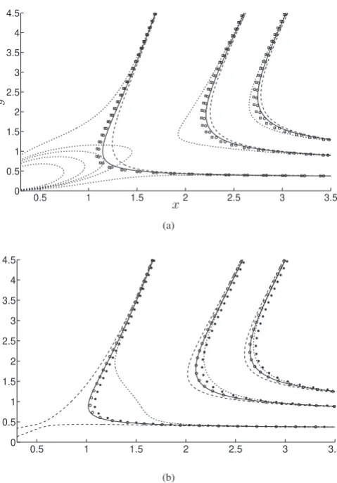
The streamlines are given inFig. 2(a) for the case of a shear thinning fluid andFig. 2(b) for a shear thickeningfluid. The Newtonian solution is plotted together with thefirst and second order perturbation terms and the Shanks transform. To prove the validity of the expansion, Eqs. (2)and(3)are solved numerically using thefinite element solver COMSOL Multiphysics. A Newtonian velocity field was imposed far from the corner with the moving and no-slip boundary conditions ap-plied along the walls. Note that thefirst and second order terms quickly become invalid as the corner is approached, and thus only provide an appropriate correction from the zeroth order solution far from the corner. The Shanks transform improves convergence remarkably well for the shear thickeningfluid even as the corner is approached, despite the underlying assumptions becoming invalid. However, for the shear thinningfluid, the Shanks transform does not perform as well. These results indicate that for shear thinning fluids the streamlines under-shoot those of the Newtonianfluid, and that for shear-thickeningfluids, the streamlines overshoot the Newtonian solution. A possible ex-planation for this is that as the viscosity of the system is reduced through shear thinning, the wall exerts a small shear stress on thefluid. Afluid element must be then closer to the moving wall before it can be dragged offhorizontally.

4. Near corner approximationE≫1

To further extend the domain in which analytic results can be found, we will now focus on the region closest to the corner where the shear rates are extremely large. We now consider the asymptotic series as

→ ∞

∼ + − + − + ⋯ ψ ψ₀ 2ψ ψ

1 4 2

E E (28)

and

+ − ∼ − − + − − + ⋯

γ γ κ γ

[1 2 2˙ ] n 1˙n 1 n ˙n .

1 3 3

n 1 2

E E E (29)

Comparing orders ofE,the momentum equation gives ∇ × ∇_{·{ ˙γ}n−_{γ˙ }}=_{0: at order (} n−_),

0 1

0 O E 1 (30)

∇ × ∇_·{(n−_{1) ˙ ˙γ γ}n− _γ˙ +_γ˙n− _γ˙ +_{κ γ˙}n−_{γ˙ }}=_{0: at order (} n−_).

1 0 2 0 0 1

1 1 0 3 0 O E 3

(31) The zeroth order solution,ψ0, was obtained previously by Riedlerand Schneider[12], whereψ₀=Rg θ₀( )andg0is given by the expression

⎜ ⎟

= ⎛ ⎝

− ⎞

⎠ + g θ K θ

K α θ K θ K α θ

( ) 1 ( )

( ) sin

( ) ( )cos , 0

1

1

2

1 (32)

where

∫

∫

= ′ ′ ′ = ′ ′ ′

K θ1( ) θ F θ( ) cos( )θ dθ, K θ( ) θ F θ( ) sin( )θ dθ,

0 2 0

n

n

1

1

(33) with

= ⎧

⎨ ⎪

⎩ ⎪

− − <

− =

− − >

∞

∞

∞ F θ

n n θ θ n

θ θ n

n n θ θ n

( )

sin( (2 ) ( )) for 2,

( ) for 2,

sinh( ( 2) ( )) for 2. ₍₃₄₎

The parameterθ∞is found by requiring thatK α2( )=0. The solution for

g0 can be obtained from analysis of the momentum equation which reduces to

− + ″ − + ″ = + ″ − + ″ ″

n n( 2)g g n (g g ) [g g n (g g )] ,

0 0 1 0 0 0 0 1 0 0 (35)

where ′ denotes differentiation with respect to θ. The solution for + ″

g₀ g₀ gives

+ ″ + ″ =

⎧

⎨ ⎪

⎩ ⎪

− − <

− =

− − >

∞

∞

∞ g g g g

A n n θ θ n

A θ θ n

A n n θ θ n

sgn( )

sin( (2 ) ( )) for 2,

( ) for 2,

sinh( ( 2) ( )) for 2, n

0 0 0 0

(36) where _A− =_{K α n n( ) (} −₂₎

1

n n

1 1

2 . Eqs. (32) and(33) can then be ob-tained by the method of variation of parameters and applying the constraintsg₀(0)=g α₀( )= ′g α₀( )=0andg₀′(0)=1. We will now focus on the perturbed partial differential equation (PDE)(31). On dimen-sional grounds we will seek a solution of the formψ₁=R g θ3 ( )

1 . One can

examine the region where the series is valid prior to the calculation of g1. If one assumesg1isO(1),and thatψ0andψ1increase asRandR3, respectively, then the first order solution loses its uniformity again when ₋ψ

ψ 0 2 1

E isO(1),i.e. whenRis

− ( 1)

O E . This corresponds to the same region as that where the Newtonian solution loses uniformity. In effect, we have sandwiched the region of non-uniformity from above and from below. The zeroth andfirst order terms for the shear rate and rate of strain tensors can be written as

= + ″ = ⎛

⎝ ⎜

+ ″

+ ″

⎞

⎠ ⎟

= ″ + ″ − = ⎛

⎝ ⎜

′ ″ −

″ − − ′

⎞

⎠ ⎟

− −

γ R g g R g g

g g

γ R g g g g R g g g

g g g

γ

γ

˙ , ˙ 0

0 ,

˙ ·sgn{( )}·( 3 ), ˙ 4 3

3 4 .

0 1 0 0 0 1

0 0

0 0

1 0 0 1 1 1

1 1 1

1 1 1 (37)

Substituting(37)into the 1st order momentumEq. (31)leads to the ODE

− + ″ ″ − + + ″

+ − + ″ ′

+ − − + ″ ″ − + + ″ =

− −

−

− −

d

dθ n g g g g κ g g n d

dθ g g g

n n n g g g g κ g g

{ ( 3 ) }

8( 3) { }

( 2)( 4){ ( 3 ) } 0,

n

p n

n

n

p n

2

2 0 0 1 1 1 0 0 2

0 0

1 1

0 0 1 1 1 0 0 2

(38) where

= ″ +

κp sgn{(g0 g0)} .κ (39)

g1is subject to the homogeneous conditions

= ′ = = ′ =

g₁(0) g₁(0) g α₁( ) g α₁( ) 0. ₍₄₀₎

Eq. (38)has a regular singular point wheng₀+ ″ =g₀ 0. FromEq. (36), it can be seen that this occurs whenθ=θ∞. We now shift the coordinate system so thatθ=θ∞maps toθ=0. One would expect difficulties to arise in the formulation asγ˙→0,as the expansion for the viscosity(29) will clearly fail. This problem is rectified inSection 5. As no exact closed form analytical solution to Eq. (38) can be found except for special parameter choices (seeAppendix A), we proceed by seeking the homogeneous solution to(38). Tofind the general solution we will seek a series in the form

̂

∑

= = ∞

+ g θ( ) g θ( ) ,

i

i i β

1

0 (41)

[image:4.595.43.283.50.394.2]

and use the series expansion Fig. 2.A plot of the streamlines for (a)n=0.5and (b)n=1.7,with a corner angle of

=

α π

2. Thefirst and second order perturbation solutions are given by the dashed and

+ ″ ∼ ⎡ ⎣ ⎢ + − − − − ⎤ ⎦ ⎥ +

(

+

)

≠

g g K α θ θ n θ n n θ

θ n

sgn( ( ) ) 1 ( 2) 6

( 2) (2 5) 360

for 2 , n

0 0 1 2

2 4 6 1 n 1 A O (42) which is obtained from Eq. (36) and we define

= _{K α( )}−_{n 2}−_n

1 1 n n

1 2

1 2

A . Substituting the series (41) and (42) into (38), it is seen that for a non-trivial series expansionβmust satisfy

− − + − + =

β β( 1)(nβ (n 1))(nβ (2n 1)) 0. (43) The roots of(43)allow one to construct the four linearly independent solutions which can be written for ∉

n 1 as ⎜ ⎟ ⎜ ⎟ ⎜ ⎟ ∼ + + − − +⋯ ∼ ⎛ ⎝ + − − − − + − + − − − + ⋯⎞_⎠ ∼ ⎛ ⎝ + − + + + + − − − + − + + + + + + + + ⋯⎞_⎠ ∼ ⎛ ⎝ − − + + + + + − − + − + + + + + + + + ⋯⎞_⎠ + +

k θ n

n θ

k θ n

n θ

n n n n

n n n θ

k θ n n n

n n θ

n n n n n n n

n n n n θ

k θ n n n

n n θ

n n n n n n

n n n n n θ

1 3

2

25 51

8(3 1) ,

1 1

6 (14 27)

(2 1)

128 2136 7258 8001 2025

120(2 1)(3 1)(4 1) ,

1 1

2

( 2)(2 33 25)

(2 1)(3 1)

( 2)(48 116 220 18095 11362 31171 8170)

360(2 1)(3 1)(4 1)(5 1) ,

1 6 53 65 42

6(3 1)(4 1)

336 716 6516 47975 93312 16385 11380

360(2 1)(3 1)(4 1)(5 1)(6 1) .

n

n

1 2 4

2 2

4 3 2

4

3 1

1 2

2

6 5 4 3 2

4

4 2

1 3 2

2

7 6 5 4 3 2

4

(44) The homogeneous solution is unphysical forθ< 0 as for certain values ofnthe solution may be complex, moreover, the functionsk3andk4are never smooth at the pointθ=0. The way to overcome this is by se-parating the solution into two domains forθ> 0 andθ< 0, and then matching the solution across the boundaryθ=0. The homogeneous equation, obtained by settingκp=0inEq. (38), is invariant under the

transformationθ→ −θ. We thus separate the solution into

= ⎧ ⎨ ⎩

+ + + >

− + − + − + − <

+ + + +

− − − −

g A k θ B k θ C k θ D k θ θ A k θ B k θ C k θ D k θ θ

( ) ( ) ( ) ( ) 0,

( ) ( ) ( ) ( ) 0.

homo

1 2 3 4

1 2 3 4 ₍₄₅₎

We later show that _A+=_A−_,B+= −_B−_,C+=_C− _andD+_{= −D}−_{. The} inhomogeneous solution can again be found by seeking a Frobenius series solution given by

⎜ ⎟ = ⎛ ⎝ − − − − + − + − − − − − + ⋯⎞_⎠ − −

k θ θ n

n

n n n n n n

n n n n θ

sgn( )

2(2 1)

(12 60 187 81 2) ( 2)

12(4 1)(3 1)(3 2)(2 1) .

p 1 2 n

1

4 3 2

2 A

(46) Note that the singularity atn=2 arises as a result of the change of behavior of the zeroth order solution and must be considered sepa-rately. The singularities atn=1

2in thefirst term andn= , , 1 4

1 3

3 2in the

second term can be resolved using by the introduction of logarithmic terms [18].Eq. (46)gives the complete outer-solution, however, for matching across the boundary we need only consider the limit asθ→0. The leading order behavior could be found more directly without the need to obtain the full solution (seeAppendix B). Evaluation of either method results in the expression

∼ ⎧ ⎨ ⎪ ⎪ ⎪ ⎩ ⎪ ⎪ ⎪ − − − + → − − − + → − − + − − −

(

)

(

)

ψ n

n K α n n R θ θ

n

n K α n n R θ θ

2(2 1) ( ) ( 2)

homogeneous terms

as 0 ,

2(2 1) ( ) ( 2) ( )

homogeneous terms

as 0 . 1 1 1 3 2 1 1 3 2

n n n

n n n

1

2 21

1

1

2 21 1

(47) The asymptotic behavior ofg0asθ→0 can be found by solving (42) and keeping the first term on the left hand side of the series. The equation can be integrated to give a solution which can be written in terms of hyper-geometric functions. However, for the case of ∉,

n

1

if

we take the leading order term in the Taylor series wefind

∼ + + ± + ⋯ → ±

±

∞ ±

(

+

)

g sin(θ θ ) C ( θ) n , as θ 0,

0 0 2

1

(48) where the first term, which arises from the homogeneous term in Eq. (36), does not contribute to the shear rate and_C±

0 is given by

= ±

+ +

±

C n K α

n n sgn( ( )) (2 1)( 1). 0

2 1 A

(49) We can see that the stream functionψbehaves asO(1)where thefirst order term has fractional powers of_θ1+n1_,θ2−n1_{. The stream function is}

uniformly valid ifθ→0 for2− >0 n

1

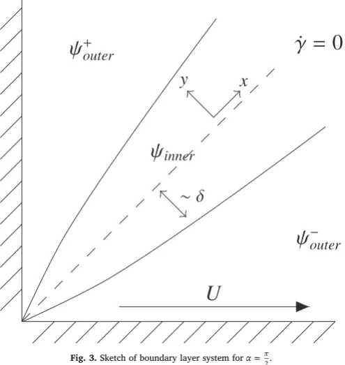
. However, the shear rate and thus the stress tensor, are not uniformly valid for anyn> 0. It is clear that the solution breaks down along the lineθ=0 due to the shift from power law to Newtonian behavior. To analyze this change in physical behavior we assume that a boundary layer of unknown thickness exists aroundθ=0. We adopt Cartesian variables as polar coordinates offer no advantage, and we use the approach proposed by Renardy[19]. We chose our Cartesian system such thatx, yare parallel and perpendicular to the lineθ=0 respectively (Fig. 3).1 Let us now suppose that the boundary layer has thicknessδwhich leads to the introduction of the scalings y=δY x, =X. Note that the polar coordinates are related to the Cartesian coordinates byR∼X,θ∼δY/X, which will be used later in the matching process. In the inner boundary layer, the scaling of the stream function remains unknown, and we adopt an arbitrary scaling

= + + ′

ψ_inner Δ Ψ0 g(0)X δg(0) ,Y (50)

whereX, YandΨareO(1) and the orders ofδandΔ0remain to be determined. The last two terms inEq. (50)are included to account for the homogeneous term inEq. (48). Physically these terms represent a constant velocityflowing into the boundary layer, but have no effect on the momentum equation. Under these scalings it useful to note that the velocity gradients are given by

= − = − − = = − −

ux vy Δ0δ1Ψ ,XY vx Δ Ψ ,0 XX uy Δ0δ 2Ψ .YY (51) Physically theXderivatives should be small compared to theY deri-vatives as no change in the velocity gradients occurs in the outer so-lution in this direction. In Cartesian variables, the momentumEq. (7) can be written as

⎜ ⎟ ⎛ ⎝ ∂ ∂ − ∂ ∂ ⎞ ⎠ + ∂ ∂ ∂ − =

x y τxy x y(τyy τxx) 0.

2 2 2 2 2 (52) Substituting(50)into(7)and keeping the lowest order terms, onefinds ∇ × ∇_{· (1}

{

+ _Δδ−_{Ψ )}− _Δδ−_{Ψ e e}

}

=_0.

YY YY x y

2 0 2 4 2

0 2 n 1

2

E ₍₅₃₎

We now argue that within this layer there must be a transition between Newtonian and non-Newtonian behavior. In the power-law region, the shear-dependent term _E2 2γ˙ _{dominates the +1 term in the viscous}

Eq. (1), and likewise in the Newtonian case the+1term dominates over the shear term, thus for a transition to occur we require that they are both of the same order. Hence _Δδ−

0 2

E must beO(1), giving thefirst condition,_Δ = −_δ

0 E 1 2. Substituting forYand keeping the leading order

terms gives ⎡

⎣ + ⎤⎦ =

−

(1 Ψ )YY ΨYY 0, YY

2 n21

(54) which we will refer to throughout as“the boundary layer equation”. We can readily see that this PDE permits similarity solutions of the form

=_{X ϕ X}

(

− _Y

)

Ψ b b₂ .

(55) The constantbis determined by requiring that the inner solution must match up to the outer solution _ψ=_Rθ2+n1∼_δ2+n1_X−

(

1+1n

)

_Y2+n1_{. This}

requires thatb−b

(

2+_n

)

= −

(

1+_n

)

, 2

1 1

which leads tob=2+2n. The boundary layer equation subsequently becomes

= ⎡

⎣ + ″ ″⎤⎦ ″

=

+ −

X ϕ χ ϕ ϕ

Ψ 2 2n ( ), (1 2)n21 0,

(56) where′denotes differentiation with respect toχ, with _χ=_X− +(1 n)_Y.

This matching condition is satisfied if_ϕ∼_χ2+n1 _asχ→∞. Integrating

twice and setting the constant term to be zero we obtain the non-linear second order ODE

+ ″ϕ − ϕ″ =A χ

[1 2] b .

n 1

2 ₍₅₇₎

Though no general closed form solution toEq. (57)can be found, the asymptotic behavior can be readily seen. First let us consider the case as χ→∞, whereby the left-hand side of (57) must become large. This requiresϕ′′to become large and thus the+1term becomes negligible, hence [1+ ″ϕ2] − ϕ″ ≈(ϕ″)n

n 1

2 _{. Thus ϕ″ ∼χn}1 _{as χ→∞ and hence} ∼ +

ϕ χ_n1 2,_{which is the correct matching condition. For the inner} solu-tion as χ→0 the left-hand side of Eq. (57)must be small and thus ϕ′′≪1. Hence + ″ ″ ≈ ″

− ϕ ϕ ϕ

[1 2]n21 _{. Thus, the inner behavior is as} ϕ∼χ3_{. We can see the change in behavior by solving the boundary} layer equation(1+ ″ϕ2) −ϕ″ =χ

n 1

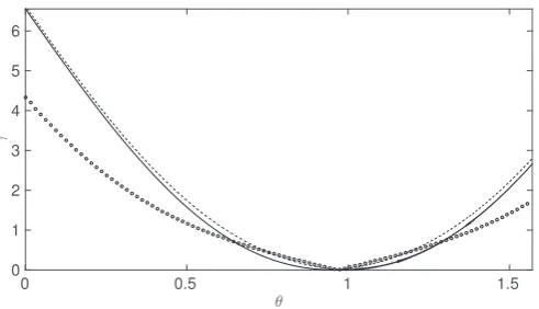
2 _{numerically. This was achieved by} integrating ϕ″ =Z x( ) using a second orderfinite difference scheme, whereZ(x) is the inverse function ofP x( )=(1+x2)(n−₂1)x,_{which was} found using the Newton Raphson method. The solution is shown in Fig. 4, along with the inner and outer approximations. This permits us to examine the boundary layer behavior as the Newtonian limit is ap-proached. If thefluid is everywhere Newtonian, there is no change in behavior and thus there must be no boundary layer. One might have expected that the size of the layer would tend to zero, however, wefind its size in fact tends to_E−1_{. In the Newtonian limit, we actuallyfind the}

inner behaviorχ3_{, and the outer behavior χ}2+n1_{,coincide and thus no}

change in behavior occurs.

We can now see that behavior of the inner solution far from the boundary can be written in terms of the outer variablesx, yas

∼ −

(

+

)

+ = − + − + + ψ_inner Δ0X 1 n Y n Δδ nx n y n.

1 2 1

0 (2 1 ) (1 1 ) 2 1 (58)

Thus, for the orders to match, we require that _Δ =_δ

(

+

)

0 2 n

1 . By

combining this with thefirst condition,_Δ = −_δ,

0 E 1 2 we get the explicit

scaling of the boundary layer_δ=_E−n_{andΔ =} − n+

0 E (2 1). Physically, we

see that this new scaling is applicable when_E∼_γ˙−1_{as to be expected.}

This scaling could alternatively have been deduced from looking at the form of the behavior of the outer solution. The behavior of the zeroth order term it is as_rθ2+n1 _{and for the} fi_{rst order term it is as}

−2 3 2_{R θ}−n1

E forn< 2. By considering the ratio of these terms we see that the solution loses its uniformity when

= =

+

− −

− Rθ

R θ ( R θ) (1). n n

2

2 3 2 n n

n

1

1

2

E E O (59)

As we considerRto beO(1) this gives the required scaling for θas −

( n)

O E . The scaling forψbecomes apparent whilst expressing thefirst term in the outer series in terms of the scaledθ, i.e. if_θ=_E−n_Θ,then

= − + +

ψ R n Θ

0 (2 1) 2 n

1

E . Likewise, one can see that the similarity variable appears as the ratio of the power-law and viscous correction terms. In Section 5, we will formally match the boundary layer equation to the outer solution.

The boundary layer occurs when_Y∼_E−n_{. The scaling suggests that} asngrows large this boundary layer region becomes infinitely small, with the inner stream function scaling also becoming smaller, though we laterfind that for asymmetricflows an additional layer of width_E−2

occurs which dominates forn> 2 . This is discussed inSection 5.3. However, as mostfluids exhibit shear thinning properties, oftenn< 1 and consequently this layer would be much smaller than the_E−n_layer.

5. Matching

5.1. Leading order

As two of the boundary conditions are applied in the regionθ> 0, and the other two in the regionθ< 0, to get a complete solution we must match the solutions over the boundary layer. Wefirst consider the case ofn< 2. The case ofn> 2 is considered inSection 5.3. The free parameters of the outer solution(47)can be matched to the inner so-lution to obtain a soso-lution defined across the whole domain. As the inner scaling can be derived from consideration of where the outer shear rate loses its uniformity, this suggests that the zeroth andfirst order terms in the outer series match to the lowest order in the inner series. We now formally match the leading order inner solution to the outer solutions. Considering the expansion for the outer solution(57) and using the series approximation for largeϕ′′, we obtain

″ ″ + − ″ ″ + ⋯=

−

−

ϕ ϕ n 1 ϕ ϕ A χ

2 .

n

n

p

1

3

[image:6.595.309.557.55.208.2]

(60) We can construct the inverse series, by means of iteration, tofind Fig. 3.Sketch of boundary layer system forα=π

2.

Fig. 4.Solution for + ″ ″ =

−

ϕ ϕ χ

(1 )

n

2 21 _{given by the solid line with the inner,χ}3_{, and}

outer,_χ2+_n1_{,behaviors given by the dotted and dashed lines, respectively, for the case of}

=

n 3

[image:6.595.40.288.59.321.2]

∑

″ = ∼ ∼ − −

+ = ∞

− −

−

{

}

( )

ϕ f χ β χ A χ A χ n

n A χ

χ

( ) sgn( ) ( ) 1

2 ( )

, m

m n m

n _{p p p} n

n

0

1 2 1

3

n

1

O ₍₆₁₎

which integrates to give

∫ ∫

= + + ″ ″ ′ ∼ + + + +

′

ϕ A Bχ χ χ f χ( )dχ dχ (A Int) (B Int χ)

0 0 1 2

(62)

+ + − −

+ ⋯ → ∞

+

− − χ n

n n A A χ

χ n

n A A χ

χ sgn( )

( 1)(2 1)sgn( )

sgn( )

2(2 1)sgn( )

as ,

p p n p p

n n

2

2 1

1

2 1 n

1

(63) where Int1, Int2 are the order 1 contributions which arise from the contribution to the integral forχ not large. These are calculated nu-merically by

∫

= ∞

(

′ − ′ ′

)

′

Int2 f χ( ) sgn(A χp )(A χp ) dχ , 0

n1

(64)

∫

∫

∑

= ⎛

⎝ ⎜

⎜ ″ ″ − _{+ −}

− ⎞

⎠ ⎟ ⎟ ′

∞ ′

= + − <

+ −

(

)

Int f χ dχ β χ

Int dχ ( )

1

. χ

m n nm

m

n m n

n nm

1

0 0

0 1 1 2 0

1 2

1 1 2

2

(65) Via Van Dyke’s matching rule [20] if A= −Int B1, = −Int2 and

= − −

A A K α n n

sgn( p) pn1 1( )1 21n( 2) ,21n or equivalently Ap= −

− K α K α n n sgn( ( )) ( )n ( 2 ) ,

1 1

1

2 12 and assgn( )θ =sgn( ),χ then the outer limit ofϕis given by

= −

+ +

−

− − + ⋯

−

+

− −

(

)

ϕ n θ K α n n

n n χ

θ n

n K α n n χ

sgn( ) ( ) ( 2) ( 1)(2 1) sgn( )

2(2 1) ( ) ( 2) ,

n

n

2

1 1 2 1

1

1 2 1

n n

n n

1

2 21

1

2 21

(66) which matches exactly with the inner behavior of the inhomogeneous terms in the outer solution obtained previously(47)and(48). Reverting back to polar coordinates and introducing the scaling forr,Ωallows one to incorporate the Newtonian effects to leading order from use of the composite approximation to zeroth order with the expression

=_{r g θ}

(

−_C+_θ + _θ

)

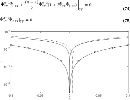
+_r+ _{ϕ r}−_θ Ω_{comp 0}( ) ₀ 2 n1sgn( ) 2 2n ( n ).

(67) The composite expansion gives an expression that is uniformly valid over the troublesome zero shear layer (Fig. 5), though it is important to note that it does not resolve the loss of uniformity due to the radial decrease in shear rate. The composite streamlines are plotted inFig. 6 along with the power-law solution and complete numerical solution for a Carreaufluid as withFig. 2. One can see that thefirst order solution correctly captures the behavior of the Carreau fluid for small r, al-though the lost of uniformity is apparent as the radial distance grows.

5.2. Matching homogeneous terms: second internal boundary layer

To correctly apply the boundary conditions the constants + + + +

A ,B ,C ,D must be matched to the corresponding terms in the lower domain, _A−_,B−_,C−_,D−_{. Using the aforementioned scaling leads} one to look for an inner solution of the form

= + +

+ + + +

∞ − ∞ − + +

− − + − + − +

ψ sin(θ )X cos(θ )Y X ϕ

Ψ Ψ Ψ Ψ ,

inner n n n

A n B n C n D

(2 1) 2 2

2 ( 2) ( 3) (2 3)

E E

E E E E (68)

whereΨA,ΨB,ΨC,ΨDmap tok1,k2,k3,k4, respectively. The details are

given in[18]. After matching to the outer solutions the inner shear-rate is found to have inner behavior

= + +

+ + +

− + − + − + + −

− + + −

A X Y n

n C X D n n

n X Y

Ψ ( 3)

( 1)(2 1) .

YY n b n n n

n _n

(2 1) (1 ) ( 3)

2

2 1

(2 3)

2

1 1

E E

E

The leading order shear rate behaves as_E−(2n+1)_{Y,whereas the}

homo-geneous terms give rise to a shear rate_E−(n+3)_{. This results in a loss of}

uniformity when_Y∼_En−2_{which arises because the point of zero shear}

no longer occurs whenY=0as predicted by the pure power-law so-lution. Instead, the point of zero shear has been shifted due to the presence of the anti-symmetricflow term. Physically this is to be ex-pected as one would not anticipate a Carreaufluid to have exactly the same point of zero shear as a pure power-lawfluid.

This leads us to propose a second inner scaling whereby_Y=_En−2_Y,

which can be written as_y=_{E Y}−2 _{in terms of the outer coordinates.}

This scaling describes purely Newtonian behavior and does not change so one can simply express(68)in terms of this scaling. The solution can therefore be written as

= + + +

+ ⎛

⎝ +

+ ⎞

⎠

+ + +

∞ − + ∞ − +

− + − +

− − +

ψ θ X A X θ B X

n

n C X X

n n

n X D

sin( ) ( cos( ) )

1 2

( 1)(2 1)

6 ,

n _n n

n _n

inner 2 3 4 2

7 2 1 2 2 2 3

9 2

1 1 3

E Y E Y

E Y Y

E Y

(69) which leads to a uniformly valid shear-rate. By considering the limit as

→ −

[image:7.595.312.558.53.194.2]

Y 0 in conjunction with symmetry arguments leads to the matching constraints_A+=_A−_,B+= −_B−_,C+=_C−_andD+_{= −D}−_{. We now have} a smooth uniform approximation, which completes the matching. Fig. 5.The shear rate along the contourr=1forn=0.45,α=π

2is plotted. The outer

[image:7.595.311.555.576.709.2]

power-law solution (solid line), the inner boundary solution (circular markers) and the composite curve (dashed lines) are shown.

The effect of the inner boundary layers is shown inFig. 7, where the shear rate is plotted forfixedr. The effect of the second inner layer of shifting the point of zero shear can be observed.

5.3. Strong shear thickeningfluids.

In the case ofn> 2, the previous matching is no longer valid. This can be explained by considering the expression for the shear rate taking thefirst order terms in the outer series,

= + ⎛

⎝ −

−

+ ⎞

⎠

− + − + −

γ C Rθ R C θ n n θ

˙ 1

2 (1) .

n n

outer 0 2 3 1

1 1

n

1

E O

(70) Thefirst term in the brackets arises fromk3in the homogeneous solu-tion(44), with the constant_C+_{derived from the boundary conditions,} and the second from the inhomogeneous term. Forn> 2, as_θ→_{0 ,}+ _we see that the contribution from the homogeneous term is larger than that of the inhomogeneous term and the solution loses its uniformity before

∼ −

y _E n_{. From analysis of the ratio of the two terms we propose an} inner scaling of the form _y=_E−2_Y,ψ∼E− −4 n2_Ψ_{. This new scaling is}

required as the innermost boundary layer (of thickness_E−2_{) is now}

larger than the previous outer layer (of thickness_E−n_{). Upon using this} scaling and keeping only thefirst order terms, the momentum equation reduces to

= ((Ψ ) )YY 0.

n YY

 ₍₇₁₎

IntegratingEq. (71)gives

= + ∼⎧

⎨ ⎩

+ → ∞

+ →

− − −

− − C Y D

C Y n D C Y Y

D n D C Y Y

Ψ ( )

as ,

as 0,

YY pn p

p p p n

p p pn

1 1 1

1 1 n

n n

n n

1

1 1

1 1



(72) whereCPandDpcan be functions ofX. We can immediately see that the zero shear rate no longer occurs at Y=0. We now set

= − − −

(

+

)

Cp K α1( ) 1n21n(n 2)21nX 1 n

1

and_D =_nC−_{C X}+ − p pn 1 2 n

1

and match the other homogeneous solutions and the inhomogeneous term. Thus, we seek a solution of the form

= + + + +

+ +

∞ − ∞ − − − −

− − − +

ψ sin(θ )X cos(θ )Y Ψ Ψ Ψ

Ψ Ψ ,

n _{A B}

n D n I

inner 2 4

2 _{2 4}

6 2 6 2

E E E E

E E

  

  ₍₇₃₎

whereΨ , Ψ , A B andΨDmatch tok1,k2andk4. We again setΨA=A X+ 3 and_Ψ =_{B X Y}+

B 2

 _{and note thatΨ}_{C is excluded ask3has already been} matched in (72). The introduction of ΨI is required to match to the inhomogeneous term. The equations forΨDandΨIare given by ⎡

⎣

+ − + ⎤

⎦ =

− n −

Ψ Ψ ( 1)

2 Ψ (1 2Ψ Ψ ) 0,

YY n

I YY YY

n

YY I YY YY

1 2

    

(74)

= −

[ΨYY Ψ ] 0. n

D YY YY

1

  ₍₇₅₎

The additional+1term forΨIresults from expanding the term in the constitutive equation for viscosity,1+ 2 2γ˙ ≈1+ 2(ψ _YY)

inner 2

E E . ForΨI

the cross term isO(1),hence the inclusion of the+1term in(74). If we again consider the limit asY→∞, ΨYY∼C Yp n,

1

andEq. (74)can be written as

⎡

⎣ ⎤⎦ = ⎡_⎣⎢−

− _⎤

⎦ ⎥

− −

Y n

nC Y

Ψ ( 1)

2 .

n _{I YY}

YY p

n

YY

1 1 1 2

(76) The inhomogeneous term gives rise to a particular solution

= −

− −

− −

(

+

)

−

n

n K n n X Y

Ψ

(2 1) ( 2) ,

I ₁ 21n n n n

1

2 1

1 2 1



(77) which correctly maps to the outer solution. To obtain the inner solution behavior of(74), we note thatΨYY∼Dpn

1

 _{asY→0, and thus}

= ⎡ ⎣

− − ⎤

⎦ n

n D

[Ψ ] ( 1)

2 ,

I YY YY p

YY

n

1 

(78) hence the inner behavior ofΨI∼ − − D Y

n n p

1 4

2 n1

 _{. The analysis forΨ}_D fol-lows in a similar manner. Thus we obtain the inner solution

= + + +

+ − −

+ + +

∞ − + ∞ − +

− − − +

− − − +

ψ θ X A X θ Y B X

D Y n

n D Y

n n

n X D Y

sin( ) ( cos( ) )

1 2

1 4 ( 1)(2 1)

6 .

inner

n p n p

n n

2 3 4 3

4 2 2 6 2 2

6 2

2

1 1 3

n1 n1

E E Y

E E

E

(79) The above expression is uniformly valid, and the same matching con-ditions as before for_A+_,A−_,⋯_,D−_{still apply. So what has happened to} the layer of order _E−n_{? In fact, it has been shifted to where}

+ =

C Ypn Dp 0. The breakdown can be seen to occur here asΨYY∼Yn1,

and_Ψ ∼_Y−

I n

1

whereY =Y+D Cp/ pn. This breakdown can befixed in the same way as before.

6. Decaying effects

6.1. Newtonian case

In the far-field approximation, we found that the Carreau effects decayed like_r−1_{,(asr→∞) but a key question is whether or not this}

will be the dominant correction? The problem can be seen by noting that expression(15)is not the only solution to the biharmonic equation that satisfies the boundary conditions. In fact, there are infinitely many solutions that can be written in the formψ∼ψ + ∑_λr f θλ ( ),

0 whereλis

an eigen-value which, for a corner of angleα, satisfies

− ± − =

λ α λ α

sin(( 1) ) ( 1)sin( ) 0, (80)

where ± is positive for an even mode and negative for an odd mode [2]. As we requirefinite behavior in the farfield we have the condition

ℜ(λ) < 0. These extra degrees of freedom come from the fact that the behavior near to the corner is not specified.

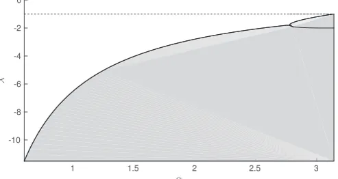
The eigen-modes decay slower than the leading order Carreau ef-fects ifR( )λ < −1. We canfind the eigen-values by numerically solving (80). The leading order negative eigen-value is shown inFigs. 8and9. Thus, the farfield Carreau analysis is applicable for α< 2.2 rad and further deviation shown inFig. 2(a) cannot be explained by the ex-citation of a slowly decaying eigen-mode.

6.2. Non-Newtonian case

For the near-corner power-law system, it is also important to in-vestigate whether Carreaufluid effects would be masked by the decay of farfield disturbances. We thus search for a stream-function in the form

= + + + …

ψ rg θ( ) r gλ ( )θ r g ( )θ ,

λ λ λ

[image:8.595.40.287.520.711.2]

0 1 1 2 2 (81)

where1<λ1<λ2< …andg0is the solution toEq. (32). The additional terms are the modes that are excited from behavior far from the corner region. As we are only interested in the slowest decaying modeλ1, for ease of notation we letλ=λ1,and as shear thinningfluids are much

more prevalently found in nature, we present the eigen-value problem only for n< 1. Substituting (81)into(7)and(8)and taking leading order inrasr→0 gives rise to the eigen-value problem

⎧ ⎨ ⎩

−∂

∂ + + − − −

⎫ ⎬ ⎭

⎛

⎝ − − ″ − −

⎞ ⎠

− − − ⎡

⎣ − −

′⎤ ⎦ ′

= ∞

−

∞ −

θ λ n λ n

n n n θ θ g λ λ g

λ n λ n n θ θ g

( 1 )( 1 )

sin( (2 ) ( )) ( ( 2) )

4( )( 1) sin( (2 ) ( )) 0.

n

λ λ

n λ

2

2

1 1

1 1

(82) Classically such eigen-value problems are solved numerically by using a shooting method. However, one can see that locally, aroundθ=θ∞,the non-differentiable functions cause difficulties with ODE solvers. We thus decided to solve the problem using a Frobenius series approach. To simplify the problem we assumed thatsin( n(2−n) (θ−θ∞))is well approximated by n(2−n) (θ−θ∞). Under this assumption the gen-eral solutions can be found analytically with the eigen-value problem being expressed as a root-solving problem. The root-solving is per-formed using a Newton–Raphson method and the initial value is found by iterating from the Newtonian solution. The effect ofnon the New-tonian even and odd modes is shown in Fig.10, although it should be noted that forn≠1 the eigen-functions are no-longer strictly even or odd. This is to be expected as, due to non-linearity, the eigen-functions couple to the leading order behavior, which does not have such a symmetry. One can see fromFig. 10that forn< 0.76,ℜ(λ) < 3.

7. Conclusions and discussion

Wefind that for a Carreaufluid in a wall driven corner the radial scale determines the dominant physics of the problem, therefore we introduce the scaling thatris_{O E(} −1_{). Far from the corner (E→0) the}

solution can be readily calculated and that the result correctly predicts the overshoot and undershoot of streamlines for shear thinning/thick-ening behaviors, respectively, though the solution is no longer valid for small r. However, the far from wall approximation will eventually breakdown due to the inertia terms becoming appreciably large. In the limit of largeE,that is highly shear dependent behavior, we found that the system can be modeled as a pure power-law solution in part of the domain. However, this solution breaks down along the line of zero shear and a novel boundary layer equation is required to overcome this problem. The thickness of the region in which the solution breaks down is found to be of the order_E−n_{,with another change in behavior atE}−2_.

This suggests that the stresses of shear thinningfluids with small power-law indexnnear a region of low shear rates could vary greatly from those predicted by a pure power-lawfluid. The need to separate into different length scales arises in the driven cornerflow problem due to the fact that the moving wall boundary condition forces the stream function to behave asr, which precludes a self-similar solution as the shear rate is radially dependent. However, if one considers theflow caused by constant shear stress (Fig. 11), as performed by Moffatt[2]in the Newtonian case, there is no radial dependence on the shear rate and a global self-similar solution can be found. We seek a solution of the form_ψ∼_{τ μ}−_{r f θ( )}

0 ₀1 2 whereby the stress tensor components reduce to

= ′ = − = ″

τrr 2μf τθθ, τrθ μf , (83) with the shear rate as given byEq. (9),

= − ″ + ′

γ˙ τ μ0 0 (f 4f ) ,

1 2 2 12

[image:9.595.313.555.56.191.2]

(84) Fig. 8.Newtonian eigen-values plotted againstαfor an odd eigen-function (symmetric

[image:9.595.42.289.59.190.2]

flow) excitation. The shaded region indicates where the Carreau correction is applicable.

Fig. 9.Newtonian eigen-values plotted againstαfor an even eigen-function (anti-symmetric flow) excitation. The shaded region indicates where the Carreau correction is applicable.

Fig. 10.The real part of the eigen-value for the non-Newtonian problem (Eq. (82)) at an angle ofα=π

[image:9.595.41.336.577.733.2]

whence the viscosity simplifies to

= + − ″ + ′ −

μ μ₀(1 (Γτ μ0 ₀1 2) (f 2 4f 2)) . n 1

2

(85) The momentumEq. (7), after introducing a similar scaling approach as used in(4)to remove intertia, reduces to the non-linear ODE

+ ″ + ′ − ″ + + ″ + ′ − ′ =

{

}

{

}

d

dθ f f f

d

dθ f f f

(1 ( 4 )) 4 (1 ( 4 )) 0.

2

2

2 2 n21 2 2 n

1 2

(86) WhenEq. (86)is solved subject to a constant shear stress being applied at some angleαand a no-slip condition on the bottom wall it gives the constraints

= = ′ = + ″ + ′ − ″ =

f(0) f α( ) f (0) 0, (1 (f ( )α2 4 ( ) ))f α2 n₂1f ( )α 1. (87) As no analytic solution could be found we solved (87) using the shooting method in conjunction with a Runge–Kutta 4 solver. The

results are presented inFig. 12. One might have considered applying a similar matching approach to that used for the driven corner problem to this system. However, one can see fromEq. (84)that zero shear can only occur when there is no curvature and gradient inf. From the graph inFig. 12, we can see that this scenario never occurs, thus no break-down will occur.

The regions of applicability for both the near-field and far-field analysis were found. The far-field Carreau correction is found to be of greater importance than the eigen-modes for angles less than ≈2.2 rad. However, for larger angles, the decay from the near corner effects are more prevalent. A similar study was performed for the near-region. We concluded that, other than for weakly shear-thinningfluids, the far field eigen-modes are more important except for in the boundary layer region.

Acknowledgment

This work was supported by funding from the EPSRC grant EP/ I019790/1.

Appendix A. Exact solution for power-law correction.

For the parameter choicen=3the general solution for the correction to the power-lawEq. (38)can be found in terms of tabulated functions. For =

n 3,the governing equation simplifies to

⎜ ⎟

⎛ ⎝

+ ⎞ ⎠

+ ″ ″ − + + ″ =

d

dθ 1 {3(g g ) (g 3 )g κ gp g } 0.

2

2 0 0 2 1 1 0 0

(A.1) This can be solved by the same means asEq. (35)which leads to the exact solution

= − ∞ + − ∞ + +

g₁ Asinh( 3 (θ θ )) Bcosh( 3 (θ θ )) CI θ1( ) DI θ2( ). (A.2)

The functionsI1andI2are given by:

∫

∫

= − −

− − −

− −

∞ ∞

− −

∞ ∞

I θ e e θ θ θ θ dθ

e e θ θ θ θ dθ

( ) sinh ( 3 ( ))sin( )

sinh ( 3 ( ))sin( ) ,

θ θ

θ θ

1 3 3

2 3

3 3 2₃

(A.3)

∫

∫

= − −

− − −

− −

∞ ∞

− −

∞ ∞

I θ e e θ θ θ θ dθ

e e θ θ θ θ dθ

( ) sinh ( 3 ( ))cos( )

sinh ( 3 ( ))cos( ) .

θ θ

θ θ

2 3 3

2 3

3 3 2₃

(A.4)

Appendix B. Inner behavior of the outer solution

[image:10.595.311.556.52.199.2]

The solution toEq. (38)was obtained by use of Frobenius series, and is required to give the additional terms needed to describe the behavior far fromθ=0. However, the leading order terms could be computed in a more direct manner, and as the equation appears later in the matching process we include it. If one considers the case whereθis small, then the second order derivatives dominateEq. (38). Keeping the highest order derivatives for the homogeneous and inhomogeneous parts onefinds that

Fig. 11.Sketch of the shear drivenflow problem.

[image:10.595.49.288.54.234.2]