A Study of the Sulfide Stress Corrosion Cracking in a Supermartensitic Stainless Steel by Using EIS

Int. J. Electrochem. Sci., 10 (2015) 5249 - 5263

International Journal of

ELECTROCHEMICAL

SCIENCE

A Study of the Sulfide Stress Corrosion Cracking in a

Supermartensitic Stainless Steel by Using EIS

C.J. Ortiz-Alonso1, J.G. Gonzalez-Rodriguez1,*, J. Uruchurtu-Chavarin1,J.G. Chacon-Nava2

1

Universidad Autonoma del Estado de Morelos-CIICAP, Av. Universidad 1001, Col. Chamilpa, 62209-Cuernavaca, Mor., México

2

Centro de Inv. En Materiales Avanzados, Miguel de Cervantes 108, Chihuahua, Chih., Mexico

*

E-mail: ggonzalez@uaem.mx

Received: 10 March 2015 / Accepted: 4 May 2015 / Published: 27 May 2015

In this work, an attempt for using electrochemical impedance spectroscopy (EIS) to study the development of sulfide stress corrosion cracking (SSCC) in a UNS S41425 supermartensitic stainless steel has been done. Slow strain rate tests have been used to achieve this goal. It was found that when the steel is susceptible to SSCC, both the Bode modulus and phase angle decreased as straining increased between 0.1 and 10 Hz. Electric circuit was used to simulate the EIS data and it was found that both the diffusion layer resistance inside and the crack charge transfer resistance decreased after the yielding point.

Keywords: Corrosion cracking, stainless steel, electrochemical impedance spectroscopy.

1. INTRODUCTION

application [7,8]. Generally they are used in several corrosion conditions and when economical aspects are a critical issue, since they offer better mechanical and corrosion properties than carbon steels [9-12].

Electrochemical techniques such as electrochemical noise (EN), which is a non-destructive technique, has been extensively used to detect stress corrosion cracking susceptibility of metallic alloys in different environments [13-23], obtaining current or potential fluctuations and were related with the nucleation and propagation of stress corrosion cracks. However, the use of Electrochemical Impedance Spectroscopy (EIS) measurements in the study of SCC has been more limited. For instance, Oskuie [24] used EIS to study the susceptibility to SCC of a X-70 pipeline steels with the aid of a widely used techniuwe called Slow strain rate testing (SSRT) in a solution containinh high pH bicarbonate. EIS tests at a fixed potential were conducted simultaneously at regular peidods of time in order to elucidate the changes associated with the SCC. Both type of Bode for cracks were calculated. They found the range of a suitable frequency were the detection of cracks. Bosh [25] applied the EIS technique in the monitoring SCC in a stainless steel sample exposed to a high temperature aqueous environment. The impedance of a cracked surface was described with a model which could distinguish between a flat electrode surface and an electrode surface with cracks. They used three types of experiments: (1) Sensitized Type 304 SS by using sSlow strain rate tests on in a 5 N H2SO4 + 0.1 M

NaCl solution, (2) 304 type stainless steel by using the constant load tests in a boiling (±110 0C) acidified sodium chloride solution, and (3) 304 typs stainless steel with the aid of the slow strain rate tests in an oxygen containing solution of 0.01 M Na2SO4 at 300 0C. the phase shift between the two

samples could be related to the stress corrosion cracking process. Lou [26] usied slow strain rate tests applied EIS measurements in order to study the susceptibility of carbon steel to SCC in simulated fuel-grade ethanol (SFGE) . They found that the Phase angle decreased during an active crack growth. When the steel was susceptible to SCC, the frequency at maximum phase angle increased around 1 Hz. Thus, the goal of this paper is to use EIS measurements to detect SSCC of a supermartensitic stainless steel in an H2S-containing environment.

2. EXPERIMENTAL PROCEDURE

Table 1. Chemical composition of tested steel. (wt. %).

C Mn Si Cr Ni Mo S P Cu N Fe

0.02 0.75 0.3 13.5 4.7 1.7 0.0003 0.016 0.07 0.07 Bal.

testing at a strain rate of 1.00 x 10-6 s-1. Testing solution includes a heated, de-aerated 3% NaCl solution, whereas H2S was produced by reacting 3.53 mg L-1 Sodium Sulfide (Na2S) with 1.7 mg L-1

Acetic acid at 25, 40, 60 and 80 0C. SCC tests were carried out at the free corrosion potential value. The susceptibility to SCC was measured by the loss in ductility in terms of the percentage reduction in area (%R.A) with the aid of following equation:

100 .

.

% x

A A A A R

i f

i 

 [1]

where Ai and Af are the initial and final area respectively. A susceptibility index to SCC (ISCC)

was calculated as follows:

air NACE air

SCC

A R

A R A

R I

. . %

. . % . .

% 

 [2]

where %RAair and %RANACE are the percentage reduction in area values in air and in the

NACE solution respectively. A value of ISCC close to 0 means immunity towards SCC, whereas a value

close to 1 indicates a high susceptibility. Tensile-fractured specimens were examined by a JEOL scanning electron microscope (SEM). EIS tests were carried out at the Ecorr value during the straining

by using a signal with amplitude of 10 mVSCE and a frequency interval of 0.1 Hz-30 kHz by using a

PC4 300 Gamry potentiostat. Measurements were obtained during straining by using a graphite rod as auxiliary electrode, a saturated calomel electrode (SCE) reference electrode with a Luggin capillary bridge. Polarization curves were performed in a potentiodynamic way at a sweep rate of 1 mV s-1 in an AC Gill potentiostat once the free corrosion potential value (Ecorr) was stable. A saturated calomel

reference electrode (SCE) was used as reference electrode wereas a graphite rode was the auxiliary electrode. Cylindrical specimens were encapsulated in commercial epoxic resin with a total exposed area of 1.0 cm2. Potentiodynamic polarization curves were performed. Corrosion current values, Icorr,

were calculated by using Tafel extrapolation method.

3. RESULTS AND DISCUSSION

The effect of the temperature in the polarization curves is shown in Fig. 1, where it can be seen that at room temperature, i.e. 25 0C, the steel displayed an active-passive behaviour with an Ecorr value

around -755 mVSCE and an Icorr value close to 0.002 mA cm-2. The passive zone started around -700

mVSCE and ended at a pitting potential value close to -200 mVSCE after which a transpassive zone could

be found. When the temperature increases up to 60 or 80 0C, the Ecorr values increased up to 590 and

-550 mVSCE respectively whereas the Icorr was very similar for both temperatures, close to 0.1 mA cm-2,

but the steel still displayed an active-passive behaviour. The passive zone was narrower than that found at 25 0C, but the pitting potential remained the same at the three different temperatures. It has been reported that in H2S-containing solutions, the corrosion process of iron and steel is generally

make these films more protective than those found on iron or steels. The addition of Mo improves the pitting resistance and enhances passivity.

Figure 1. Effect of the temperature in the polarization curves for UNS S41425 supermartensitic stainless steel in H2S-containing 3.5 % NaCl solution.

Figure 2. Effect of the temperature in Iscc value for UNS S41425 supermartensitic stainless steel in

H2S-containing 3.5 % NaCl solution.

This is so for several factors which produce a passive film more resistant, making easier the transition from an active-to-passiver behavior by reducing the anodic peak, and slowing down the

1E-5 1E-4 1E-3 0.01 0.1 1 10 100

-1600 -1400 -1200 -1000 -800 -600 -400 -200 0 200 400 600

E

(

mV

)

Current density (mA cm-2)

250C

600C

800C

400C

20 30 40 50 60 70 80 90

0.4 0.5 0.6 0.7 0.8 0.9 1.0

Iscc

dissolution rate for the naked substrate making it more difficult to sustain the local chemistry necessary for localized corrosion. By combining Mo with Ni, the outer layers of the passive film has been shown [31] to be enriched whereas the inner passive layer is made of Cr. Additionally, Mo is considered to form MoS giving protectiveness in presence of H2S. This stops the access of H2S to the under-layer,

consisting of solely chromium oxide. The formed films become more porous and less protective with an increase in the temperature and thus, it will occur an increase in the corrosion rate.

Figure 3. Micrographs of specimens fractured in a H2S-containing 3.5 % NaCl solution at a) 25, b)60

and 800C.

The susceptibility towards SCC for the a supermartensitic stainless steel in the H2S-containing

NaCl solution is given in Fig. 2, where it can be seen that the steel is practically immune to SCC at 25

0

Figure 4. Nyquist curve for UNS S41425 supermartensitic stainless steel in H2S-containing 3.5 %

NaCl solution at 25 0C during the SSRT.

Figure 5. Bode plot in the Impedance-frequency format for UNS S41425 supermartensitic stainless steel in H2S-containing 3.5 % NaCl solution at 25 0C during the SSRT.

Nyquist diagram for specimen fractured at 25 0C, which was immune to SCC, is shown in Fig. 4, where it can be seen that, before applying any stress, data displayed two semicircles: one at high and intermediate frequency values, and another one at lower frequencies, indicating a corrosion process controlled by the charge transfer reaction. As stated above, in H2S-containing solutions, the corrosion

process of iron and steel is generally accompanied by the formation of iron sulfide film. Thus, one of the observed loops in Fig. 4 corresponds to the formed sulfide film, whereas the second loop

0 200 400 600 800 1000 1200

0 200 400 600 800 1000 1200

0 200 400 600 800 1000 1200 1400 1600 0 200 400 600 800 1000 1200 1400 1600 Zim ( Oh m cm 2)

Z_re (Ohm cm2)

Before straining Z im ( Oh m c m 2 )

Z_re (Ohm cm2)

25 0C

Before yielding point

Yielding point

UTS

Final fracture

0.1 1 10 100 1000 10000

200 400 600 800 1000 1200 1400 1600 1800 Imp e d a n c e ( Oh m c m 2 ) Frequency (Hz) Before straining Before yielding point

Yielding point

UTS

Final fracture

corresponds to the double electrochemical layer. As soon as the straining started, the two observed semicircles remained throughout the tests, but their diameters decreased as compared to the unstrained specimen. During the first hours of testing and before reaching the yielding point, the semicircles diameter increased due to film growth due to corrosion activity. After the yielding point, the semicircles diameter decreased until the final fracture, due to the deterioration of the film. Bode plot in the Modulus format, Fig. 5, showed that the modulus was higher for the unstressed condition, and it decreased when the straining begun, diminishing as the strained continued throughout the test, confirmed by the Nyquist results, indicating that the growth of the external formed sulfide film is affected by the straining.

Figure 6. Evolution of the impedance modulus with time at different frequency values for UNS S41425 supermartensitic stainless steel in H2S-containing 3.5 % NaCl solution at 25 0C during

the SSRT.

The evolution of the impedance modulus with time at different frequency values (0.1, 1 and 100 Hz) is shown in Fig. 6, where it can be seen that, generally speaking, the impedance value increased as the frequency decreased and, at the same frequency value, it remained more or less constant as time increased. On the other hand, Fig. 7 shows that before applying any stress, the phase angle increased as the frequency decreased, remaining more or less constant between 100 and 0.1 Hz, where it started to decrease with a further decrease in the frequency.

0 10 20 30 40 50 60 70

10 100 1000 10000

Imp

e

d

a

n

c

e

mo

d

u

lus

(

Oh

m c

m

2 )

Time (h)

1 Hz

100 Hz 0.1 Hz

Figure 7. Bode curve in the Phase angle-frequency format for UNS S41425 supermartensitic stainless steel in H2S-containing 3.5 % NaCl solution at 25 0C during the SSRT.

Figure 8. Evolution of the phase angle with time at different frequency values for UNS S41425 supermartensitic stainless steel in H2S-containing 3.5 % NaCl solution at 25 0C during the

SSRT.

As the straining started, the phase angle was lower than that for the unstressed condition at frequency values higher than 1 Hz; below this frequency, the phase angle values were higher than those in the unstressed condition. For the stressed condition, the phase angle values were virtually the

0.1 1 10 100 1000 10000

-60 0 60

P

h

a

s

e

a

n

g

le

(

0 )

Frequency (Hz)

25 0C

Before straining Before

yielding point

Yielding point UTS

Final fracture

0 10 20 30 40 50 60 70

10 20 30 40 50 60 70

P

h

a

s

e

a

n

g

le

(

0 )

Time (h)

1 Hz

100 Hz

same regardless of the deformation of the steel. This is confirmed in Fig. 8, which shows the evolution of the phase angle with time at different frequency values. This figure shows that at the same frequency, although there is a decrease in the phase angle during the first hours of straining, it remained more or less constant as time elapsed until the specimen reached its final fracture.

Figure 9. Nyquist curve for UNS S41425 supermartensitic stainless steel in H2S-containing 3.5 %

NaCl solution at 80 0C during the SSRT.

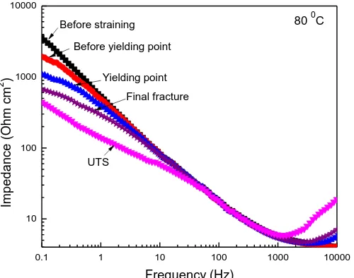
Figure 10. Bode plot in the Impedance-frequency format for UNS S41425 supermartensitic stainless steel in H2S-containing 3.5 % NaCl solution at 80 0C during the SSRT.

0 500 1000 1500 2000

0 500 1000 1500 2000

0 500 1000 1500 2000 2500 3000 3500 4000

0 500 1000 1500 2000 2500 3000 3500 4000 Zim ( O h m c m 2)

Zre (Ohm cm2) before straining

0 5001000150020002500300035004000

0 500 1000 1500 2000 2500 3000 3500 4000 Zim ( O hm cm 2)

Zre (Ohm cm

2 ) 0 Zim ( Oh m c m 2 )

Z_re (Ohm cm2)

80 0C

Yielding point

Final fracture

UTS

Before yielding point

0.1 1 10 100 1000 10000

10 100 1000 10000 Imp e d a n c e ( Oh m c m 2 ) Frequency (Hz) Before straining

Before yielding point

Final fracture

UTS

80 0C

Figure 11. Evolution of the impedance modulus with time at different frequencies for UNS S41425 supermartensitic stainless steel in H2S-containing 3.5 % NaCl solution at 800C during the

SSRT.

Specimen fractured at 80 0C increased its susceptibility towards SCC, as indicated data from Fig. 2. Nyquist diagram for unstressed specimen, Fig. 9, displayed, what looks like un unfinished semicircle with its centre at the real axis; as soon as the specimen was strained, data displayed a semicircle at high and intermediate frequencies, together with a second loop at lower frequency values. One of the observed loops in Fig. 9 corresponds to the formed sulfide film, whereas the second loop corresponds to the double electrochemical layer. It can be seen that as the specimen was strained and time elapsed, the semicircle diameter decreased except at the final fractured, where the semicircle diameter increased again. Additionally, as time elapsed, data displayed only one semicircle, which might be due to the crack opening and growth and the degradation of the external sulfide film due to the applied stress. This is reflected in the Bode-modulus plot, Fig. 10, the total impedance at the lowest frequency increased as time elapsed, indicating the external sulfide film degradation and crack growth. The change in the impedance modulus with time at different frequency values is plotted in Fig. 11, where it can be seen that at 100 Hz, this parameter remained practically constant as time elapsed. However, at lower frequency values, i.e. 1 and 0.1 Hz, the impedance modulus decreased as the applied stress increased, just as reported by Oskuie and Bosch [24,25] and related this fact to an increase in the crack size and/or in the number of secondary cracks.

The Bode-phase angle plot, practically remained constant with time in a frequency window of 10-1000 Hz or so, Fig. 12; for frequency values lower than 10 Hz, the phase angle decreased as the specimen was strained, except when it reached the final rupture, where the angle phase increased again. Thus, Fig. 13 shows that at 100 and 1000 Hz, the phase angle remained more or less constant during the straining, but at 1 Hz, the phase angle decreased as the specimen was strained. In all cases

0 10 20 30 40

10 100 1000 10000

Imp

e

d

a

n

c

e

mo

d

u

lus

(

Oh

m c

m

2 )

Time (h) 0.1 Hz

1 Hz

100 Hz

the phase angle increased once the specimen was ruptured, which might be due to repassivation and film growth on the crack corroded surface [25]. Such a decrease in phase angle can be correlated to the corrosion cracking process, as reported elsewhere [24, 26, 34, 35] for instance, for the SCC of carbon steel in fuel-grade ethanol.

Figure 12. Bode curve in the Phase angle-frequency format for UNS S41425 supermartensitic stainless steel in H2S-containing 3.5 % NaCl solution at 80 0C during the SSRT.

In Fig. 13 it can be seen that at higher frequencies than 1000 Hz, the phase angle remained constant as time elapsed, but at 100 and specially 1 Hz, the phase angle decreased after 10 hours, as the steel was strained. It can be seen from Figs. 5 and 10 that at 0.1 Hz, the decrease in both the impedance modulus and the angle phase changes in slope after 20 hours more or less, once necking has started [32] which can be an indicator of passive layer deterioration in the necking area on the gauge of the tensile specimen.This effect has been related by Oskuie, Bosch and Lou [24-26] to an increase in the crack size. Here, once again, these results are consistent with the reported results by other researchers [24, 25] who have reported that cracks can only be detected at frequencies lower than 10 Hz, which the authors proposed as the suitable frequency range for detection of the cracks.

In order to interpret its EIS response during a stress corrosion crack, many factors can be involved such as crack tip behavior, crack wall behavior, solution chemistry in the crack, and crack propagation path. For the interpreatation of the EIS data, it is a common practice to use Randles circuit (Fig. 14) where Rsol, Rw, Rct and Cdl are the solution resistance, the resistance of a Warburg´s element,

charge transfer resistance and double layer capacitance respectively. However, in our experiments,

0.1 1 10 100 1000 10000

-90 -60 -30 0 30 60 90

P

h

a

s

e

a

n

g

le

(

0 )

Frequency (Hz)

Before straining

Yielding point

Final fracture UTS

80 0C

SCC is a dynamic process which involves changes in both crack geometry and electrochemical activity.These changes are contributed by crack growth, crack tip activity, crack wall activity including secondary cracks growth, and crack chemistry inside a single crack. Inside the crack, Rw represents the

resistance of the Warburg element or a diffusion layer.

Figure 13. Evolution of the phase angle with time at different frequencies for UNS S41425 supermartensitic stainless steel in H2S-containing 3.5 % NaCl solution at 80 0C during the

SSRT.

Figure 14. Electric circuit used to simulate EIS data at 80 0C.

Since stress corrosion cracking is a dynamic process, this should be reflected within the interval of used frequencies during the EIS experiments. The response from a higher frequency perturbation represents a faster electrochemical process, which is more close to a non-Faradaic process. The presence of a diffusional Warburg impedance in the EIS should be associated to surface concentration of an electrochemical active species changes during the AC cycle, and reflects in for example, the impedance of the cathodic reaction. At high frequencies the real and imaginary parts of the impedance

0 10 20 30 40 50

-20 -10 0 10 20 30 40 50 60 70 80

P

h

a

s

e

a

n

g

le

(

0 )

Time (h)

1 Hz

100 Hz

1000 Hz

are equal for semi-infinite diffusion. Thus, our results show that there is a frequency lower than 1Hz where the electrochemical behavior after the maximum stress is very clear. The frequency interval between 1 and 0.1 Hz represents at the best the cracking behavior in a reasonable way.

Table 2. Parameters used to simulate the EIS data at 60 0C using circuit in Fig. 17

Point Rsol

(Ohm cm2) Rw

(Ohm cm2)

Cdl

(F cm-2)

n Rct

(Ohm cm2)

Before straining 4.42 3685 15.8 0.73 70

Before yielding point

3.94 8610 24.8 0.81 435

Yielding point 3.71 12735 15 0.86 631

UTS 3.78 501 95 0.76 450

After rupture 4.45 3053 14.7 0.86 10

The changes in the shape of the Warburg impedance can be associated to the form of the pore or crack which affects the AC signal penetration within the crack [41]. Table 2 shows the parameters used to simulate the obtained EIS data for test performed at 80 0C. It can be seen that both the resistance of the diffusion layer inside the crack, Rw and the charge transfer resistance, Rct, are the

parameters which are greatly modified during the straining. Thus, It can be seen that, generally speaking, both Rw and Rct increased with time, reaching its highest value at the yielding point,

decreased at the UTS, and increased once again at the final rupture. This means that the aggressive species diffuse more easily through this layer after the yielding point; at final rupture the Rw value

increased once again, maybe because the crack walls are repassivated making more difficult the access of the aggressive species. However, the Rw values were higher than those for Rct, indicating a

diffusion-controlled process. In the literature, there are studies of the effect of H2S on iron and steel

[37-40]. These results showed that both the anodic iron dissolution and the cathodic hydrogen evolution are accelerated by H2S. Sulfide-induced SCC is a process enhanced by an anodic dissolution

process, where the access of the aggressive species including hydrogen cathodic discharge is necessary for corrosion to occur, which is in agreement with the results found in this study.

4. CONCLUSIONS

References

1. A. John Sedriks, “Corrosion of Stainless Steels”, John Wiley and Sons, Inc., Princeton, NJ, 1979. 2. T. Taira, K. Tsukada, Y. Kobayashi, H. Inagaki and T. Watanabe, Corrosion 37 (1981) 5.

3. H. Pircher and G. Sussek, Corros. Sci. 27 (1987) 1183.

4. G. Domizzi, G. Anteri and J. Ovejero-Garcĺa, Corros. Sci. 43 (2001) 325.

5. L.W. Tsay, M.Y. Chi, H.R. Chen and C. Chen, Mater. Sci. Eng. 416 A(2006) 155.

6. The Institute of Materials, Corrosion Resistant Alloys for Oil and Gas Production: Guidance on General Requirements and Test Methods for H2S Service, Maney publishing, (2002) p. 9.

7. H. Marchebois, J. Leyer, B. Orlans-Joliet, Proceedings from the NACE Corrosion conference (2007), Paper 07090 2007 CP, Houston, TX, NACE International.

8. X. Li, T. Bell, Corros. Sci. 48 (2006) 2036.

9. M.D. Pereda, C.A. Gervasi, C.L. Llorente and P.D. Bilmes, Corros. Sci. 53 (2011) 3934. 10.H. Van-der-Winden, P. Toussaint and L. Coudreuse, Proceedings, Past, Present and Future of

Weldable Supermartensitic Alloys, Supermartensitic Stainless Steel, Brussels, Belgium, 2002. 11.T.G. Gooch, P. Woollin and A.G. Haynes, Proceedings, Welding Metallurgy of Low Carbon 13%

Chromium Martensitic Steels, Supermartensitic Stainless Steel, Brussels, Belgium, 1999. 12.D. Carrouge, Proceedings, Transformations in supermartensitic stainless steels”, Ph.D. thesis,

University of Cambridge, Department of Materials Science and Metallurgy, England, 2002. 13.S. Ritter and H. P. Seifert, Materials and Corrosion 64 (2013) 683.

14.R.C. Rathod, S.G. Sapate, R. Raman and W.S. Rathod, J. Mat. Eng. and Perf. 22 (2013) 3801.

15. Mathias Breimesser, Stefan Ritter, Hans-Peter Seifert, Thomas Suter, and Sannakaisa Virtanen, Corr. Sci. 63 (2012) 129.

16.C.J. Ortiz Alonso, M.A. Lucio–Garcia, I.A. Hermoso-Diaz, J.G. Chacon-Nava, A.

MArtinezVillafañe and J.G. Gonzalez-Rodriguez, Int. J. Electrochem. Sci., 9 (2014) 6717. 17. Li Jian, Kong Weikang, Shi Jiangbo, Wang Ke, Wang Weikui, Zhao Weipu and Zeng Zhoumo,

Int. J. Electrochem. Sci., 8 (2013) 2365.

18.G.L. Edgemon, M.J. Danielson and G.E.C. Bell, J. Nuclear Materials 245 (1997) 201. 19.J. Hickling, D.F. Taylor and P.L. Andresen, Materials and Corrosion 49 (1998) 651. 20.J. Kovac, M. Leban and A. Legat, Electrochim. Acta 52 (2007) 7607.

21.T. Anita, M.G. Pujar, H. Shaikh, R.K. Dayal and H.S. Khatak, Corros. Sci. 48 (2006) 2689. 22.G. Du, J. Li, W.K. Wang, C. Jiang and S.Z. Song, Corros. Sci. 53 (2011) 2918.

23.S.W. Kim and H.P.Kim, Corros. Sci. 51 (2009) 191.

24.A.A. Oskuie, T. Shahrabi, A. Shahriari and E. Saebnoori, Corros. Sci. 61 (2012) 111. 25.Rik-Wouter Bosch, Corros. Sci. 47 (2005) 125.

26.Xiaoyuan Lou and Preet M. Singh,Electrochim. Acta 56 (2011) 1835.

27.S. Arzola, J. Mendoza-Florez, R. Duran-Romero and J. Genesca, J. Solid. State. Electrochem. 7(2003) 283.

28.T.A. Ramanarayanan and S.N. Smith, Corrosion 46 (1990) 66.

29.H. Vedage, T.A. Ramanarayanan, J. D. Mumford and S.N. Smith, Corrosion 49 (1993) 114. 30.Pengpeng Bai, Shuqi Zheng, Hui Zhao, Yu Ding, Jian Wu and Changfeng Chen, Corros. Sci. 87

(2014) 397.

31.H. Amaya, K. Kondo, H. Hirata, M. Ueda and T. Mori, Proceedings from the NACE Corrosion conference 1998, Paper 98113, 1998,CP, Houston, TX, NACE International.

32.M. Salazar, M. A. Espinosa-Medina, P. Hernández and A. Contreras, Corros. Eng. Sci. and Tech. 46 (2011) 464.

33.H. Keiser, K.D. Beccu and M.A. Gutjahr, Electrochim. Acta 21 (1976) 539. 34.R.W. Bosch, F. Moons, J.H. Zheng and W.F. Bogaerts, Corrosion 57 (2001) 532. 35.M.C. Petit, M. Cid, M. Puiggali and Z. Amor, Corros. Sci. 31 (1990) 491.

37.H.Y. Ma, X.L. Cheng, S.H. Chen, C. Wang, J.P. Zhang and H.Q. Yang, J. Electroanal. Chem. 451 (1998) 11.

38.M.A. Veloz and I. González, Electrochim. Acta, 48 (2002) 135.

39.18. H.H. Huang, J.T. Lee and W.T. Tsai, Mater. Chem. Phys. 58 (1999) 177. 40.S. Arzola and J. Genesca, J. Solid State Electrochem. 8 (2005) 197.

41.D. D. Macdonald, Electrochim. Acta. 51 (2006) 1376.