Principal Geodesic Analysis in the Space of Discrete Shells

This is a repository copy of Principal Geodesic Analysis in the Space of Discrete Shells.

White Rose Research Online URL for this paper:

http://eprints.whiterose.ac.uk/132588/

Version: Accepted Version

Article:

Heeren, Behrend, Zhang, Chao, Rumpf, Martin et al. (1 more author) (2018) Principal

Geodesic Analysis in the Space of Discrete Shells. Computer graphics forum. pp. 173-184.

ISSN 0167-7055

https://doi.org/10.1111/cgf13500

[email protected]

https://eprints.whiterose.ac.uk/

Reuse

Items deposited in White Rose Research Online are protected by copyright, with all rights reserved unless

indicated otherwise. They may be downloaded and/or printed for private study, or other acts as permitted by

national copyright laws. The publisher or other rights holders may allow further reproduction and re-use of

the full text version. This is indicated by the licence information on the White Rose Research Online record

for the item.

Takedown

If you consider content in White Rose Research Online to be in breach of UK law, please notify us by

Principal Geodesic Analysis in the Space of Discrete Shells

B. Heeren1∗_{, C. Zhang}2∗_{, M. Rumpf}1_{, and W. Smith}2

1_{University of Bonn, Institute for Numerical Simulation, Germany} 2_{University of York, Department of Computer Science, United Kingdom}

[image:2.595.53.556.234.417.2]

1 3 5 7 9 11 13

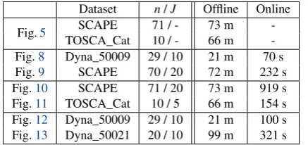
Figure 1:We show how to learn nonlinear, physically plausible modes of shape variation (bottom right) from a set of highly varying training shapes, which can be used for projection onto a low dimensional submanifold and thus sparse representation by a small set of weights. This model can be used to solve problems such as reconstruction of dense body shapes from motion capture markers (top) providing compressed animations for the reconstructed shapes via time sequences of the weights (bottom left) even when the captured data is sparse, noisy and comes from a different body shape. (Training data: 50 meshes of Dyna [PMRMB15]; Key parameters: K=4, J=10).

Abstract

Important sources of shape variability, such as articulated motion of body models or soft tissue dynamics, are highly nonlinear and are usually superposed on top of rigid body motion which must be factored out. We propose a novel, nonlinear, rigid body motion invariant Principal Geodesic Analysis (PGA) that allows us to analyse this variability, compress large variations based on statistical shape analysis and fit a model to measurements. For given input shape data sets we show how to compute a low dimensional approximating submanifold on the space of discrete shells, making our approach a hybrid between a physical and statistical model. General discrete shells can be projected onto the submanifold and sparsely represented by a small set of coefficients. We demonstrate two specific applications: model-constrained mesh editing and reconstruction of a dense animated mesh from sparse motion capture markers using the statistical knowledge as a prior.

Categories and Subject Descriptors(according to ACM CCS): I.3.5 [Computer Graphics]: Computational Geometry and Object Modeling—Physically based modeling

1. Introduction

Compact models of the shape variability of a class of 3D objects are useful in a wide range of analysis and synthesis applications across graphics and vision. Such statistical models learnt from data

provide constraint for analysis problems, compress high dimen-sional data to a low dimendimen-sional space and ensure plausibility of

synthesised results. Specifically, they can be used for non-rigid reg-istration, reconstruction from incomplete, noisy or 2D data, mesh editing, performance-driven animation and deformation transfer. To meet these applications, we address in this paper a number of important challenges:

⊲

First, many important sources of shape variability are highly nonlinear. For example, nonrigid deformation (such as articula-tion, bending, and stretching) and nonlinear shape changes (such as weight variation or shape differences between individuals).

⊲

Second, models should be physically plausible so that unrealis-tic shapes are avoided and to enable meaningful interpolation be-tween and extrapolation beyond the training samples.

⊲

Third, deformations must be modelled independently of rigid body motion. Methods that rely on factoring out rigid body motion by alignment require a choice of alignment metric, the choice of which influences the final model. Moreover, for nonrigid deforma-tions a meaningful rigid alignment may not exist.

The natural concept to deal with these requirements is a Rie-mannian shape manifold. The key ingredient for our model is a discrete geodesic (i.e. a geodesic path discretised in time) in the space of discrete shells (a triangle mesh-based approximation of the thin shell physical model). From this starting point, we propose time-discrete statistics on manifolds and make the following key contributions (summarised in the flowchart):

Input data

(I) Fréchet mean via opti-mising a sum of squared distances

(II) Gram’s matrix based on shell objects and polar formula

1

2

3

MJ

(IV) Projection operator P:

1 scaling

2

local projection 3

rescaling (III)J

princi-pal variations as weighted shell averages spanning sub-manifoldMJ

Applications: mesh editing (left) and model fitting (right)

(I) Starting from a set of input shells, we define in Section4a dis-crete geodesic average (i.e. Fréchet mean) as the minimiser of the sum of squared discrete geodesic distances to the input shapes. (II) Then, we use the polar formula for scalar products to introduce an approximate Gram matrix defined directly on discrete shapes and not as usual on infinitesimal shape variations. (III) Given the eigen-vectors, principal variations are defined as weighted shell averages

[ ]

=

{ }

[image:3.595.52.290.352.636.2]

(a) (b)

Figure 2:Key properties of the discrete shell model: equivalence classes of discrete shells[s]incorporating rigid body motion in-variance (a), with a physically sound bending (left) and membrane (right) energy density (b).

on the manifold. They are the nonlinear counterpart of (infinitesi-mal) principal components and span a finite dimensional subman-ifold (cf. Section5). (IV) Arbitrary shells can be projected onto this submanifold to provide low dimensional representations. This projection can be used to constrain the admissible set of shapes in different shape optimisation applications. In Sections6and7we exemplarily use the model for mesh editing and dense reconstruc-tion from moreconstruc-tion capture data (cf. Fig.1). The model ensures that the results exhibit physically realistic deformations while remain-ing statistically plausible.

We work directly with meshes and do not require problem-specific articulated skeletons yet our approach is able to handle many different kinds of nonlinear deformation. The discrete shell model (see Fig.2b) provides highly plausible interpolations and extrapolations within the nonlinear shape manifold, meaning that we can build rich models from very sparse training samples. The shell space in which we work is a space of equivalence classes of shapes that differ by rigid body motions (see Fig.2a) and we take special care to transfer this invariance to our time-discrete statistics. Therefore, our whole framework is rigid body motion invariant and does not require a choice of alignment metric or a preprocessing alignment step.

2. Related work

a linear space of vertex displacements and so is not rigid body mo-tion invariant and does not have an underlying Riemannian model.

Articulated models. The natural representation for deformations due to articulation is a skeleton model comprised of joint loca-tions and relative orientaloca-tions. Heap and Hogg [HH96] extended classical 2D landmark-based statistical modelling into the artic-ulated domain by building linear models over joint angles rather than vertex positions. For 3D shapes, skeletons are used to deform dense surface models (usually meshes) via a process known as skin-ning [LCF00]. In their Shape Completion and Animation of People (SCAPE) framework, Anguelov et al. [ASK∗_{05] learn a combined}

pose and deformation model and a model of the variability in body shape. A skeleton is used to drive mesh deformation using a method based on deformation transfer [SP04] and variations in body shape are learnt using a linear model of bodies in a standard pose. The Dyna model [PMRMB15] is built on top of SCAPE and adds a linear dynamics model whose coefficients depend upon the skele-ton pose. The SMPL model [LMR∗_{15] shows that pose-dependent}

blend shapes can depend linearly on the rotation matrices of the skeleton joints yet still achieve high realism of pose dependent shape and dynamics. A drawback of all of these approaches is that articulated models must be handcrafted for a specific object class and cannot capture general deformations.

Triangle deformation models. A popular approach is to build models based on the statistics of triangle deformations [ACPH06, HLRB12,CLZ13]. Instead of being trained to reproduce the input meshes directly, they are trained to reproduce the local deforma-tions that produced those meshes. Unlike elastic models, these are not physically-motivated. Sumner and Popovi´c [SP04] express deformation in terms of affine transdeformation and a displacement -the same as -the deformation model used in SCAPE. Sumner et al. [SZGP05] used deformation gradients for mesh-based inverse kinematics. Hasler et al. [HSS∗_{09] use a nonlinear representation of}

triangle deformations with 15 DoF which captures the relationship between pose and shape. Freifeld and Black [FB12] derive a 6D Lie group representation of triangle deformations with no redun-dant degrees of freedom. None of these approaches are rigid body motion invariant. Fröhlich and Botsch [FB11] additionally intro-duce a bending term, expressing deformations in terms of changes to geometric quantities (triangle edge lengths and the dihedral an-gle between adjacent trianan-gles). Gao et al. [GLL∗16] introduce a rotation-invariant mesh difference representation in which plausi-ble deformations often form a near linear subspace. The deforma-tions produced by all of these approaches will not in general be real-isable by a connected triangle mesh. Hence, these models require a further step to solve for the mesh that best fits the desired deforma-tions, which might be unsatisfactory from a theoretical standpoint.

Riemannian shape modeling. There have been numerous at-tempts to cast shape modelling or statistical shape analysis in a Riemannian setting; e.g. [FLPJ04,Pen06,KMP07]. Kilian et al. [KMP07] showed how to compute geodesic paths between tri-angle meshes using a metric that measures changes in tritri-angle edge lengths. Frequently, the underlying metric is based on mea-suring the lack of isometry, e.g. via a (linearised) elastic energy acting on the Cauchy-Green strain tensor of an associated

infinites-imal mesh deformation [SP04,ASK∗_{05,ACPH06,HSS}∗_09,FB12,

HLRB12,CLZ13,PMRMB15]. To avoid irregular, isometric shape deformations an additional regularisation is required. Heeren et al. [HRWW12] take a similar approach but use the discrete shell model which includes a bending term and leads to time-discrete geodesic paths with physical meaning (they minimise the dissipa-tion of thin shell elastic energy). The resulting shell space was sub-sequently further explored [HRS∗_{14] by introducing time-discrete}

versions of Riemannian concepts such as the exponential and loga-rithmic maps and parallel transport.

Shape collection analysis. The classicalstatistical shape mod-ellingapproach deals with objects represented by a configuration of landmark points. A point in Kendall’s shape space [Ken84] cor-responds to a configuration of landmarks in which rigid body mo-tion has been “factored out”. Linear Principal Components Anal-ysis (PCA) in this space is used to extract the important modes of shape variation. PCA has been extended to manifold valued data in the form of Principal Geodesic Analysis (PGA) [FLPJ04]. PGA models are now widely used. Fletcher et al. [FLPJ04] originally proposed the approach for modelling medially-defined anatomical objects. Freifeld and Black [FB12] used PGA to build statistical models on their Lie group representation of triangle deformations. Tournier et al. [TWC∗_{09] used PGA to build a statistical}

skele-ton model. Tycowicz et al. [vTAMZ18] presented a non-Euclidean statistical analysis of triangle meshes (represented by means of de-formation gradients, cf. [SP04]) and consider medical applications such as shape-based classification of morphological disorders. Be-sides modelling shape variation, PGA has also been applied to dis-tributions of probability measures using an optimal transport met-ric [SC15]. Whereas all these approaches model variability using only distances between objects, Rustamov et al. [ROA∗_{13] began}

a line of work which uses shape maps to more richly characterise differences between shapes and differences between differences. Boscaini et al. [BEKB15] showed how to reconstruct shapes from these shape difference operators, enabling shape analogy synthe-sis and style transfer. While the original shape differences opera-tor captures only intrinsic disopera-tortion, Cormen et al. [CSBC∗17] use offset surfaces to capture extrinsic distortion.

3. Preliminaries

One can consider the space of shapes, e.g. triangle meshes, as a Rie-mannian manifoldMwith a metricg. Then, for a paths:[0,1]→

Mthepath energyis given by

E[s] =

Z 1

0 gs(t)(˙

s(t),s˙(t))dt, (1)

where the velocity ˙s(_t)at time_tis an infinitesimal variation ofs(_t).

Given two pointssA,sB∈ Ma pathsminimising (1) among all

paths withs(0) =s_Aands(1) =s_Bis called a (shortest)geodesic

connectingsAandsBand we have

dist2(sA,sB) = min s(0)=s_A,s(1)=s_B

E[s]. (2)

Note that minimizers of (1) also minimize the length functional

L[s] =R₀1p_gs(˙s,s˙)dt. In contrast toL, the path energy isnot

con-stant absolute velocity, i.e. for allt∈[0,1]we have

gs_(t)(˙s(t),s˙(t)) =gs₍0₎(˙s(0),s˙(0)) =dist

2₍

s(0),s(1)). (3)

The geometric logarithm log_sAsB is defined as the initial velocity v=s˙(0)and for fixeds_A∈ Mthere is a 1-to-1 correspondence betweenvandsB (forsB close tosA). The corresponding inverse

mapping is denoted as exponential map, i.e. exp_sA(v) =sB.

Principal geodesic analysis. Let us briefly recall classical Prin-cipal Components Analysis (PCA) onRNbefore we consider Rie-mannian manifolds. For data pointss1, . . . ,sn∈RN the arithmetic average is given by

¯

s=arg min

s∈RN n

∑

i=1

ks−sik2_RN= 1_n

∑

i=1,...,n

si. (4)

Then Gram’s matrix is defined by G= 1_nDDT ∈ Rn,n, where

D∈Rn,N represents the data matrixwhose ith row is given by (si−s¯)T_∈

R1,N. In particular, the entries ofGdepend on the un-derlying (Euclidean) scalar product asGi j = 1nhs

i_−¯

s,sj−s¯i_RN.

SinceGis a symmetric and positive semi-definitive matrix we ob-tain non-negative eigenvalues{λj}j and corresponding

orthonor-mal eigenvectors{wj}j, i.e.Gwj=λjwjforj=1, . . . ,n. Finally,

the principal modes of variation of the data set{s1−s¯, . . . ,sn−s¯} are obtained viavj=λ−j1/2D

T_w

j∈RNforj=1, . . . ,n.

PCA in Euclidean space easily translates to Riemannian man-ifolds [FLPJ04]. To this end, one considers data pointss1, . . . ,sn

on the manifoldMand performs a classical PCA for the loga-rithms logs_¯sj of the input shapessj with respect to their Fréchet

average ¯s– the Riemannian counterpart of the arithmetic average. Thereby, the tangent vectoruj=log_s¯sj represents the geometric variation ofsj relative to the average ¯sin an infinitesimal sense. Here, the metricgs¯is taken into account as the scalar product on these infinitesimal shape variations. Thus, Gram’s matrix is de-fined byGi j= 1_ngs¯(ui,uj)and—as before—its spectral decompo-sition leads to the pairing(vj,λj)j=1,...,nwhich is called Principal

Geodesic Analysis (PGA).

Discrete Riemannian calculus on the space of shells. Rumpf and Wirth [RW15] introduced a discrete Riemannian calculus on Hilbert manifolds. Using (2) on consecutive pairs of interpolated shapessk=s(k/K)fork=0, . . . ,Kand the Cauchy-Schwarz

in-equality one obtains

E[s]≥_K

K

∑

k=1

dist2(sk−1,sk). (5)

Note that (5) becomes an equality iffsis already a geodesic path.

Now, the key ingredient of the discrete calculus is a functionalW: M × M →Rwhichlocallyapproximates the squared Riemannian distance, i.e.

W[s,s˜] =dist2(s,s˜) +Odist3(s,s˜) (6)

and replacing dist2byWin (5) leads to the definition of adiscrete path energy

E[s]:=K

K

∑

k=1

W[sk−1,sk], (7)

wheresdenotes a polygonal path with verticess_k=s(k/K) for k=0, . . . ,K. A minimiser of (7) for fixed endpoints is referred to asdiscrete K-geodesic, where the minimisation of (7) is with re-spect to theK−1 inner vertices{s1, . . . ,sK−1} ⊂ M. It is shown in [RW15] that under suitable assumptions discrete K-geodesics converge to continuous geodesics forK→ ∞.

Here, we pick up the discrete calculus on the space of discrete shells [HRWW12,HRS∗_{14]. For a fixed mesh topology a discrete}

shell can be identified with the vector of vertex positions inR3M, whereM is the number of vertices. The space of discrete shells M ⊂R3Mis then equipped with a metric which measures the en-ergy dissipation caused by infinitesimal membrane distortion and normal bending (cf. Fig.2b). The definition of the metric is based on an elastic deformation energyW[s,s˜]for thin shells needed to deforms∈ Minto ˜s∈ M. To account for the physical proper-ties of thin elastic shells,Wsplits into a membrane and a bending distortion energy (cf. Fig.2b), i.e.

W[s,s˜] =Wmem[s,s˜] +Wbend[s,s˜]. (8)

Thereby, the bending energy is taken from [GHDS03]. The dis-crete shell model is physically valid for thin shell materials. More generally, it proves useful for modelling a much wider class of ob-jects by capturing two important modes of deformation: bending and stretching. Concretely, the membrane and bending energies are defined as follows (Here, quantities with a tilde always refer to the deformed configuration):

Wmem[s,s˜] =δ

_∑

t∈T(s)

atW(Gt),Wbend[s,s˜] =δ3

∑

e∈E(s)

(θe−θ˜e)2 ae

le2,

whereT(s)andE(s)denote the set of triangles resp. edges ofs,

δ>0 is the physical thickness andW:R2,2→Ris the hyperelas-tic energy density given by Eq. (8) in [HRWW12]. Furthermore, Gt∈R2,2is a two-dimensional representation of the Cauchy Green

strain tensor of the deformation of the trianglet,at is the triangle

volume oft,leis the edge length ofe,θeis the dihedral angle at eandae=1₃(at+at′)is an area weight associated withe=t∩t′. In detail, ife0,e1,e2∈R3are edges of a trianglet, a discrete first fundamental form ontis given bygt= [e2| −e1]T[e2| −e1]∈R2,2, which yields the representationGt=g−t 1g˜t.

In order to retrieve the underlying metric one can apply Rayleigh’s paradigm by replacing strains by strain rates for a sec-ond order approximation of this energy. Indeed, due to [HRS∗_14,

Thm 1] the Hessian of (8) actually induces a Riemannian metric on the space of discrete shells modulo rigid body motions. In particu-lar, the deformation energyWrepresents a consistent approxima-tion of the induced (squared) Riemannian distance as in (6).

4. Discrete principal geodesic analysis

Based on these preliminaries we now derive a principal geodesic analysis on the space of discrete shells. The central building blocks are a discrete geodesic average, an approximation of Gram’s ma-trix, and the computation of principal modes of variation.

A critical observation of the discrete shell space introduced by Heeren et al. [HRWW12] is its rigid body motion invariance incor-porated in (8), i.e.

forR∈SO(3)(the space of rotation matrices inR3) andb∈R3. Indeed, a discrete shell is no longer a single triangular meshsbut an equivalence class of shells[s] =SO(3)s+R3, cf. the sketch in Fig. 2a. As a consequence the shape manifold Mis a space of such equivalence classes. For simplicity we stick to the notations

instead of[s]. Then tangent vectors – as they appear in the classical principal geodesic analysis – are equivalence classes as well, where the associated Lie algebraso(3)has to be taken into account. This renders the computational treatment of the shell manifold’s tangent bundle very cumbersome. In what follows, we will derive a rigid body motion invariant, discrete principal geodesic calculus based on elastic energyW. Thus, in all components of our algorithm we will solely treat discrete shells and avoid any direct tangent vector computation.

Discrete geodesic average. Lets1, . . . ,snbe discrete input shells in M. The Riemannian average on the manifold M – called Fréchet mean – is obtained by using in (4) the Riemannian dis-tance (2) in place of the Euclidean disdis-tance. Further replacingEby the discrete path energy (7) in (2) yields the definition of adiscrete geodesic average

¯

s=arg min

s∈M n

∑

i=1

min

si(0)=s, si(1)=si

E[si], (10)

where the interior minimisation is over a polygonal spider consist-ing of all polygonal pathssiconnecting the averagesi(0) =s¯and

the input shapessi(1) =_sifor_i=1, . . . ,_nas shown in Fig.4.

Ob-viously, ¯sis invariant with respect to rigid body motions due to (9).

Approximation of Gram’s matrix. Next, we substitute metric evaluations on tangent vectors in the definition of Gram’s matrix by evaluations of the squared distance directly on discrete shells, and then in a second step by the corresponding local approximation (6) as follows. Due to property (3) of geodesic paths we obtain

g(uj,uj) =dist2s¯,sj=σ−2dist2s¯,sj(σ)

≈σ−2Whs¯,sj(σ)

i

for the tangent vectorsuj=log_s¯(sj)in the standard PGA. Here,

σ>0 is some generic scaling factor andsj:[0,1]→ Mis the

geodesic connecting ¯sandsj. Note that we have used the shortcut notationg=gs¯(here and in the following). For the off-diagonal entries of Gram’s matrix we take into account the polar formula

g(uj,ui) =1 2

g(uj,uj) +g(ui,ui)−g(uj−ui,uj−ui)

and an analogous, now also in the first replacement approximate, identity

g(uj−ui,uj−ui)≈σ−2dist2(sj(σ),si(σ))≈σ−2W[sj(σ),si(σ)],

to replace evaluations of the metric with (approximative) squared distances onM. Finally, we replacesj(σ)bys₁j=I(s¯,sj,σ), where

Idenotes the discrete geodesic interpolation operator, as described in Section8, andσ=σ(K) =_K1 is a suitable choice, which retrieves the first node along the discreteK-geodesic from ¯stosj. Altogether we define the entries of an approximative Gram’s matrixG(which

1 2 4 8

10−2

10−1

100

Time discretisation (K)

RMS

relati

ve

error

Gram matrix Eigenvalues Eigenvectors

Figure 3:Convergence of the discrete Gram matrix and its eigen-vectors and eigenvalues as K→ ∞for the SCAPE dataset shown in Fig.5. We show RMS relative error, using Kmax=16as pseudo ground truth. Second order convergence is illustrated by the green triangle.

actually depends onK) as

Gi j=

W[¯s,si₁] +W[¯s,s₁j]−1₂ W[si₁,s₁j] +W[s₁j,si₁]

2nσ2 (11)

fori,j=1, . . . ,n. The additional symmetrisation in the last terms ensures symmetry ofG. Again, due to the rigid body motion

in-variance (9) the resultingGdoes not depend on the chosen rep-resentation of the equivalence classes of discrete shells. As be-fore we obtain approximate eigenvalues{λj}j and

correspond-ing (orthonormal) eigenvectors{wj}j⊂RnwithGwj=λjwjfor j=1, . . . ,n. Applying the convergence theory for the discrete cal-culus developed in [RW15] one obtains that ¯s converges to the Fréchet mean andGconverges to the original Riemannian Gram matrix1_ng(uj,ui)

i j forK→ ∞. We demonstrate this

conver-gence empirically in Fig.3.

Principal variations instead of principal components. Next, we replace the principal component (eigenmode)vjin the tangent

space at the Fréchet mean by a (nonlinear) discrete principal vari-ation on the shape manifoldM. Let us start with a straightfor-ward observation. For someα∈Rnwith∑i=1,...,nαi=1, we

con-sider the linear combinationu[α] =∑i=1,...,nαiuiof tangent vectors ui=log_s¯si. Thenu[α]can be characterized as the minimizer of the quadratic functionalu7→∑i=1,...,nαig(u−ui,u−ui). Using Taylor

expansion inσfor a givenα∈Rnthis implies that for

pσ[α]:=arg min

p∈M_i=

∑

_1,...,nαidist

2

(si(σ),p), (12)

the rescaled logarithm _σ1logs_¯pσ[α]converges tou[α]forσ→0.

Hence,pσ[α]∈ Mcan be considered as anonlinearvariation of the Fréchet mean corresponding to thelinearinfinitesimal variation

u[α]in the tangent space at the Fréchet mean.

Again, we replace dist2in (12) by its local approximationWas well assi(σ)by the discrete geodesic interpolations₁j=I(s¯,sj,σ)

withσ=1/Kand obtain

p[α]:=arg min

p∈M_i=

∑

_1,...,nαiW[s i

1,p] (13)

[image:6.595.360.510.86.179.2]

M

MJ

sm

sn sn1

sl

sl1

p−j pj

pi

¯

s

[image:7.595.77.268.82.173.2]

∂CJ

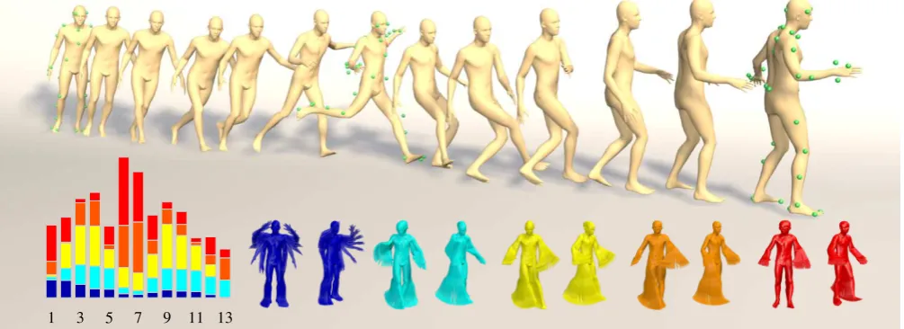
Figure 4:Submanifold MJ _{(yellow) and polyhedronC}J_{⊂ M}J (with red boundary) spanned by nonlinear combinations of prin-cipal variations{pj}j. Note that the input shapes{sk}k⊂ Mdo not lie onMJin general. The polygonal spider connecting input shapes and Fréchet mean is drawn in grey.

Figure 5: Time-discrete PGA models built on TOSCA cats [BBK08] and SCAPE [ASK∗05]. Input training shapes (yellow), mean shape (orange) and first five principal variations (green).

with special care in particular for entries ofαthat might be nega-tive. Ifαi<0 for someiwe replaceαiby|αi|andsi1=I(s¯,si,σ) by its discrete geometric reflection at ¯sinvolving extrapolation via a discrete exponential map (see Section8), i.e.I(s¯,si,−σ). This is necessary becauseWis no longer quadratic and there is no a priori control of the growth ofWfor general coefficientsαi∈R.

Thus, without this modification existence of minimisers in (13) are not guaranteed. Finally, we definediscrete principal variationsby choosingαto be the eigenvectorswj= (wj,i)i=1,...,nof the

approx-imate Gram’s matrixG, i.e.

pj:=arg min

p∈M_i=

∑

_1,...,n|wj,i| W

h

Is¯,si,sgn(wj,i)/K

,p

i

(14)

for j=1, . . . ,J, where we have rescaledwj∈Rnsuch that its

en-tries sum to 1 (which does not affect the minimiser).

Due to the convergence of the discrete Fréchet mean and the dis-crete Gram matrix we expect that for an eigenvalue of multiplicity 1 forK→ ∞the eigenvaluesλjconverge to their continuous

coun-terparts andKlogs_¯pjconverges (up to scaling) to a representative

of the corresponding principal componentvj.

Evaluation. In Fig.5we show two time-discrete PGA models (average and first five principal variations forK=4). We visualise

1 2 3 4 5 6 7 8 9 10 0

0.2 0.4 0.6 0.8 1

TOSCA Cats

0 10 20 30 40 50 60 70 SCAPE

0 10 20 30 40 50

[image:7.595.323.551.84.148.2]

Dyna

Figure 6:Model compactness with respect toWfor models shown in Fig.5(left and centre) and Fig.1(right). Number of model di-mensions on x axis, proportion of variance captured on y axis.

thejth principal variation by using the geodesic interpolation oper-atort7→I(s¯,pj,±t)to sample along the one dimensional principal

geodesic and overlay the resulting shapes. Note that they clearly correspond to nonlinear motions present in the training data. In Fig.6we show model compactness as a function of the number of retained modes for these two models and the one used in Fig.8 and Fig.12. Note that, in all three cases, we are able to compress a significant proportion of the variance into a small number of modes.

5. Submanifold projection

In this section we define a local submanifold “spanned” by the prin-cipal variations defined in (14) as illustrated in Fig.4. This is the nonlinear counterpart of the linear subspace spanned by the princi-pal components in classical PCA or standard PGA. The projection onto this submanifold returns a discrete shell which is uniquely determined by a small set of weights and approximates the input shape on the basis provided by our Riemannian statistical analysis.

Defining the submanifold. We consider (14) for the J domi-nant principal variations and also their associated reflectionsp−j=

I(s¯,pj,−1)(the sign of a principal component is arbitrary so our

submanifold includes variations in both directions). At first we de-fine the convex Riemannian polyhedron induced by the vertices {pj|j=−J, . . . ,−1,1, . . . ,J}. Discrete shells on the polyhedron

are obtained by computing “variational Riemannian” combinations of thepjfor weightsα= (α−J, . . . ,α−1,α1, . . . ,αJ)∈R2Jsubject

to∑j=−J,...,Jαj=1 andαj≥0, i.e.

CJ=

(

arg min

p∈M J

∑

j=−J

αjW[pj,p]

J

∑

j=−J

αj=1,αj≥0

)

(15)

with the notational conventionα0=0 and p0staying undefined. Note that in particular ¯s∈ CJ, e.g. forαj=α−j= 1₂ and αi=

α−i=0 ifi6= jfor an arbitrary j∈ {1, . . . ,J}as an example that

different choices ofαmight represent the same shell onCJ.

Now, the actual submanifoldMJis defined via discrete geodesic extrapolation of the convex polyhedronCJ_{using the interpolationI}

for a discrete shellp∈ CJand timest>0 (cf. Fig.4):

MJ:=nI(s¯,p,t)|p∈ CJ,t>0o. (16) We might allow for non vanishingα0andp0:=s¯, which does not alter the definition ofCJ_{. Note that (15) can also be constructed}

[image:7.595.58.287.262.402.2]

M γ=0

γ=∞

x= (xℓ)ℓ

R3L

Ploc[sloc]

P[s] sloc

s

[image:8.595.54.279.82.201.2]

MJ s∗

Figure 7:Right: Projection of an unseen shape s onto the model spaceMJ: scale s to sloc, project sloclocally toPloc[sloc]∈ CJ, and finally rescale to getP[s]∈ MJ. Left: Model fitting of s∗driven by sparse landmarks X∈R3Ldepending on fitting parameterγ>0.

The tangent space toMJat ¯sis spanned by the logs_¯pj(which

converge tovjforK→ ∞). Altogether, we get that

Klog_s¯MJ→span({v1, . . . ,vJ}) for K→ ∞.

That both principal variationspj and their reflectionsp−jare

in-dispensable to our submanifold construction reflects the fact that the infinitesimal counterpart, the principal componentsvj, generate

one dimensional geodesic subspaces and not just geodesic rays.

Defining a projection onto the submanifold. In what follows, we will derive a suitable projection of a given discrete shells∈ M on the (approximate) submanifold MJ as defined in (16). The classical Riemannian projection or projection onto the submani-fold defined as exponential map of the subspace of the tangent space spanned by the dominantJprincipal componentsv1, . . . ,vJ

would work as follows: First compute an infinitesimal representa-tionv=logs_¯sofsin the tangent space at the Fréchet mean, then

projectv(locally) onto the subspace span{v1, . . . ,vJ}via the

for-mulavJ=∑j=1,...,Jgs¯(v,vj)vjand finally compute the actual

pro-jectionP[s] =exp_s¯vJ. Note that this closed-form projection iden-tity forvJonly holds if{v1, . . . ,vJ}is an orthonormal system.

Once more the incorporation of rigid body motion invariance is a very delicate undertaking. Just replacing the metricgs¯(·,·)by the approximation used in the definition of the discrete Gram matrix in (11) does not lead to a satisfactory solution. Indeed, the expected orthogonality relationgs¯(vi,vj) =δi jholds only approximately and

that deteriorates the Gram-Schmidt orthogonalisation procedure to compute thelinearprojectionvJ (see paragraph above). Instead, we propose to perform a nonlinear projection on the approximating manifoldMJconsisting of three elementary steps:scaling,local projection, andrescaling. These steps are illustrated in Fig.7and defined in detail as follows.

[Scaling] Firstly, we scale the given shapesin order to make sure that it can be locally projected onto the polyhedronCJ(i.e. we en-sureαi≥0). This is done by means of the discrete geodesic

inter-polation (see Section8), i.e we definesloc=I(s¯,s,ρ)where

ρ:=κminjdist(s¯,pj)

dist(s¯,s) (17)

for sufficiently smallκ>0. The resulting scaling factorρis in gen-eral not a multiple of _K1. Hence, a discrete geodesic interpolation

I(·,·,t)for generalt∈Ris needed (see also Section8).

[Local projection] Secondly, we aim at computing a local projec-tion as the best approximaprojec-tion ofsloconCJ. Let us first review the

projection onto a convex setC={∑jαjqj|∑jαj=1,αj≥0}in

Euclidean space for a given set of pointsq1, . . . ,qJ∈RN. For some

arbitrary pointp∈RNthe projection can be written as

PEucl[p] =arg min q∈Cdist

2₍

p,q),

where dist2(·,·)is the squared Euclidean distance. Note that the projection coincides with the usualorthogonalprojection onto the linear space span(q1, . . . ,qJ)⊃ CifPEucl[p]is an interior point in

C(in the relative topology ofC). This formulation translates one-to-one to the local projection of a shellsloc∈ MontoCJ⊂ MJ

for smallκ, again by replacing dist2by the local approximationW. We define

Ploc[sloc] =arg min

q∈CJW[sloc,q], (18)

where the constraintq∈ CJis equivalent to

q∈narg min

p∈M J

∑

j=−J

αjW[pj,p]

J

∑

j=−J

αj=1,αj≥0

o

. (19)

In our applicationsκ= 1₂ in (17) already implies thatPloc[sloc]is

an interior point inCJ_.

[Rescaling] Finally, we rescale the local projection to define the desired projection

P[s] =I(s¯,Ploc[sloc],1/ρ). (20)

By means of this nonlinear projection method we are able to rep-resent an arbitrary shapesin terms of 2J+1 scalar variables, i.e.

α∈[0,1]2J_{to representP}

loc[sloc]∈ CJandρ>0 as in (17), which

allows for a substantial compression rate. For example, we visu-aliseαforJ=5 in Fig.1(bottom, left).

Let us emphasise that the constrained optimisation problem in-corporated in the projectionPloc does not require any treatment

of tangent vectors and is built on the rigid body motion invariant energy functionalW.

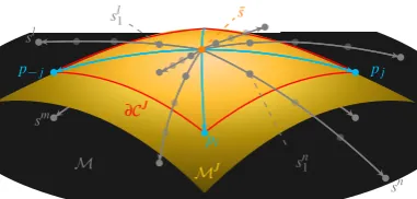
Evaluation. We show a qualitative example of submanifold pro-jection in Fig.8. The input shape (gray) is projected onto the sub-manifold obtained by building a discrete PGA model (withK=4) using the Dyna dataset (model shown in Fig. 1). We vary the model dimensionality overJ=5,11,17 and show the approximated shape in yellow. The subtleties of the shape are correctly recon-structed asJincreases, yielding a smooth residual energy. We eval-uate the generalisation ability of our model in Fig.9. We compare against [FB12] with 60 dimensions retained, the data-driven ap-proach of [GLL∗_{16] using all training shapes and the Shell PCA}

[image:9.595.57.290.88.162.2]

Figure 8:Qualitative visualisation of input shape (gray) projected onto model in Fig.1with (cols 2-4) J=5,11,17dimensions. Col 5 shows residual energy of projection with J=17.

0 0.02 0.04 0.06 0.08 0.1 0.12 0.14 0.16 0.18

0 20 40 60 80 100

Per-vertex RMS Error

%

with

error

<

x

Freifeld and Black 2012 Gao et al. 2016 Zhang et al. 2015

[image:9.595.316.551.91.261.2]

Ours

Figure 9:Leave-one-out evaluation of generalisation error on the SCAPE data set compared to [GLL∗16] (using all shapes), [FB12] (60 dimensions) and [ZHRS15]

.

6. Mesh editing via hard constraints

Our method can be used for model-based mesh editing. Assume we are given a discrete PGA model and a set ofhandle vertex posi-tions. Now, one positions (a subset of) the handle vertices manually and asks for a shell obeying the new handle positions while being a physically plausibly deformation of a shell lying on the statisti-cal submanifold. Using the submanifold projection introduced in Section5we define this shell as the minimisersof the energy

W[s,P[s]] (21)

subject to the constraint positions of the deformed handle vertices. Thus, we ask for the “closest” (in terms of the elastic energy func-tionalW) discrete shellsto the nonlinear submanifold associated with the dominantJprincipal variations of our training data. Note

that (21) is again an approximation to the actual (squared) distance.

Depending on the application one can either regards orP[s] as a solution. Indeed,sexactly obeys the prescribed handle ver-tex positions buts∈ M/ J_{in general, whereasP[s]∈ M}J_{and can}

be represented by the 2Jweightsαjbut the constraint of the

pre-scribed handle vertex positions is usually fulfilled only approxi-mately. Note that this mesh editing tool comes with a selection of a particular representativesfrom its equivalence class[s], which is determined by the handle vertex positions (as long as there are at least 3 handle vertices not lying on a line).

Fig.10 shows mesh editing results for five comparison meth-ods and our proposed approach. [SA07] and [SSP07] are classical mesh editing approaches that use only a single reference mesh. The

a b c d e

f g h i

Figure 10:Comparison of mesh editing results. (a) initial pose, (b) [SA07], (c) [SSP07], (d) [SZGP05], (e) [FB11], (f-g) [GLL∗16], (h-i) Ours (with K=4, J=20).

a b c d

Figure 11:Mesh editing with five (a-b) vs. six (c-d) handle posi-tions to be fitted, where the handle at the tail is shifted.

challenging configuration of handles causes these methods to fail dramatically. [SZGP05], [FB11] and [GLL∗_{16] are data-driven and}

use the same set of training shapes as we use to build our model. These provide more natural results but [SZGP05] and [FB11] pro-duce significant distortions and self-intersections while even the state of the art [GLL∗16] loses details, causes the arms to thin and the back to curve and deforms the head. Our result preserves de-tails and retains plausible arms and head and a straight back. Note though that the thickening of the left foot is an artefact. This is a result of the training data not including examples with such severe bending at the hip. To fit the handle on top of the foot, the solution deforms the foot rather than further bending the upper leg.

To obtain the desired result of the edit, it might be necessary to take into account sufficiently many handles as indicated in Fig.11. Here, we consider the cat model (cf.Fig.5) first with five handles and fit to modified handle positions in which the tail tip is moved. To minimise in particular the bending energy our method signif-icantly bends the whole object. This can easily be prevented by adding a sixth handle on the back of the cat (cf. Fig.11, c and d).

7. Model fitting via soft constraints

[image:9.595.89.252.216.337.2] [image:9.595.318.551.315.357.2]

[image:10.595.55.291.83.222.2]

Figure 12: Qualitative results of fitting to motion capture data. Frames from original sequence (top) shown with corresponding re-construction (bottom, using the same model as Fig.8with K=4, J=10).

on the meshs. Knowing these correspondences, we measure the mismatch of some discrete shells∈ Mand the given landmarks byFx[s] =∑L_ℓ=1kXℓ(s)−xℓk2_R3. Now, we considerW[s,P[s]]as a

prior for the identification of a reconstructed discrete shell. Hence, we seek a minimizersof the model fitting energy given by

Fx[s] +γW[s,P[s]] (22)

for some weightγ>0, which controls the proximity ofswith re-spect to our submanifold MJ for given training data, cf. Fig. 7 (left). Again this ansatz comes with a selection of a particular rep-resentativesfrom its equivalence class[s], which is driven by the data term. For the numerical solution of this problem, we make use of the following alternating scheme (based on the initial guess P[s] =s¯): First, we minimize (22) insfor fixedP[s]. If necessary, we re-computeP[s](see Sec.5) and go back to the first step. In our application this scheme quickly converges and only very few iterations already give very satisfactory fitting results. In practice, we use two iterations for the results shown.

In Figures12and13we show qualitative results of fitting to 41 markers in sequences from the CMU mocap dataset and 89 markers from MPI MoSh dataset [LMB14] respectively. Fig.12shows a result in which the learnt body model has quite different geometry to that of the performer. Note that the video frames are just shown for comparison - we use only the 3D marker data as input. Our fitted model is still able to capture the dynamic poses of the performance.

In Fig.13we compare against [LMB14]. It should be noted that this method uses a model of substantially higher complexity than ours. It is trained on 3,803 body scans in neutral pose and 1,832 body scans in dynamic poses and uses a 19 parameter skeleton model and retains up to 300 dimensions of the statistical defor-mation model (10 used in Fig.13). Our result is obtained using a model trained on 20 scans of a single person (chosen to match the body shape of the performer), is entirely mesh-based (we have no articulation model) and we also retain only 10 principal variations. Nevertheless, our results are qualitatively very similar.

Figure 13:Comparison of reconstruction from motion capture data with the MoSh model [LMB14]. Although MoSh (top) is trained on more than 5,000 scans and uses an additional skeleton model, our method with K=4(bottom) obtains similar results using 10 principal variations only, trained on a subset of 20 shapes from Dyna.

8. Computational tools

Here, we collect all algorithmic ingredients of the presented ap-proach and discuss their computational complexity.

Discrete geodesic interpolation. A discreteK-geodesic is de-fined as the minimisers of the discrete path energy (7). Thus, the unknownss1, . . . ,sK−1determining the polygonal pathssolve the

system of Euler–Lagrange equations

W,2[sk−1,sk] +W,1[sk,sk+1] =0 (23)

for k = 1, . . . ,K−1 with s0 = sA ∈ M and sK = sB ∈ M

being fixed. Here, W,i denotes the variation with respect to

the ith argument. For t = k/K for some 0≤k ≤K we set

I(sA,sB,k/K) =sk. Fort=m/Kwith arbitrarym∈Zwe define

a discrete extrapolation by an iterative scheme based on the fol-lowing induction: Assumek≥K, such thatsk−1 and sk are

al-ready known, then we compute sk+1 to be the solution of (23). Likewise, fork≤0, such thatsk and sk+1 are already known, we definesk−1 to be the solution of (23). With these extrapo-lated discrete shells at hand we define I(sA,sB,t) for arbitrary

s−1s0

sK

sA

sB t s⌊tK⌋s⌊tK⌋+1

multiplest of _K1. Finally, for general t∈Rwe de-note t(K) = tK− ⌊tK⌋ (where the floor function ⌊·⌋returns the largest inte-ger less than or equal to the argument) and defineI(sA,sB,t)as the midpointsof a discrete

3-geodesic(s⌊tK⌋,s,s⌊tK⌋+1)minimising

(1−t(K))W[s⌊tK⌋,s] +t(K)W[s,s⌊tK⌋+1], (24)

where sm= I(sA,sB,m/K) for m∈Z, as described above. In

particular,I(sA,sB,−1)defines a discrete Riemannian reflection of sB aboutsA. Computationally, we use Newton’s method to solve

[image:10.595.314.553.85.242.2]

the evaluation ofI(·,·,t)fort=k/Kwith 1≤k≤K−1. A single step of extrapolation requires to solve (23) which is obtained by solving a nonlinear system with 3Mvariables.

Discrete Fréchet mean. The most costly task is the computation of the discrete Fréchet mean ¯sdefined in (10). The degrees of free-dom (dofs) are the shells defining thenpolygonal pathssi(with

3n(K−1)Mdofs) connecting the input shellssiand ¯s(with its 3M

dofs). Each arc of the polygonal spider has to solve the system of Euler–Lagrange equations for a single discreteK-geodesic (i.e (23) for 0<k<K) and the coupling at the center is described by the Euler–Lagrange equation

0=

n

∑

i=1

βiW,2[si(1/K),s¯] (25)

with βi=1/n and si(1/K) is the first discrete shell along the

discrete path from ¯sto theith input shapesi. This coupled problem is again solved by Newton’s method.

Gram’s matrix and spectral analysis. The evaluation of the approximate Gram’s matrix (11) only consists of scaling based on the discrete geodesic interpolation and of evaluations ofW. The spectral decomposition ofG∈Rn,ncan easily be solved.

Principal variations. The computation of principal variations

pj via (14) again involves a discrete geodesic scaling as well

as computing a local weighted average similar to (25) but with non-constant weightsβi=|wj,i|.

Submanifold projection. We solve the constrained optimisation problem (18) using a Quasi Newton method. To this end, we define the objective functionalJ[α] =W[sloc,q[α]]forα∈R2Jandq= q[α]∈R3Mas the (locally unique) minimiser of

q7→ A[α,q] =

_∑

j=−J,...,J

αjW[pj,q] (26)

for fixedα0=0. To apply a Quasi Newton scheme we have to evaluate the partial derivatives ofJ with respect toαi. Forα∈R2J

the constraint on q=q[α]is given byG[α,q]:=∂qA[α,q] =0.

The solution of (18) is linked to a saddle point of L[q,α;µ]:= W[sloc,q] +G[α,q]·µ, whereµis the vector of Lagrange

multi-pliers. This leads to the nonlinear system 0=D_(q,α,µ)L[q,α;µ], i.e.

0=DqL[q,α;µ] =W,2[sloc,q] +

∑

j=−J,...,J

αjW,22[pj,q]·µ, (27)

0=DαjL[q,α;µ] =W,2[pj,q]·µ, j=1, . . . ,J, (28)

0=DµL[q,α;µ] =

∑

j=−J,...,J

αjW,2[pj,q], (29)

whereW,22denotes the Hessian with respect to the second argu-ment. By a classical result of constrained optimisation the right hand side of (28) returns the derivatives of the cost functionalJ with respect toαj. Thus, to evaluate∂αjJ we first solve the

non-linear equation (29) forqvia Newton’s method, the linear equation (27) forµvia the conjugate gradient method and then apply (28) to obtain∂αjJ[α] =W,2[|pj,q]·µ.

Multilevel algorithms. Solving a nonlinear system inO(3MnK) variables directly is inefficient at least for largerM,n, andK. For

this reason, we use a multi-resolution approach for all nonlinear optimisation problems above. First, we coarsen all of the input shapes simultaneously by applying an iterative edge collapse ap-proach based on the minimisation the quadric error metric [GH97] and computed groupwise, as in [MG03], to preserve the dense cor-respondence between input shapes. We then solve the nonlinear optimisation problem on resulting meshes with reduced resolution with<1000 vertices. Afterwards, the coarse solution is then pro-longated to the original resolution, using the prolongation scheme from [FB11]. Then a fine scale optimisation can optionally be per-formed using the prolongated result as initialisation. For a discus-sion of the accuracy of this approach we refer to [FB11, Table 2].

Furthermore, for the computation of the discrete Fréchet mean we make use of an alternating relaxation and a cascadic approach along the discrete curves of the “spider”. For the alternating scheme we first relax the average by solving (25). Secondly, we relax the

ngeodesic paths (while fixing the average) by solving (23) fork= 1, . . . ,K−1. For the cascadic approach in time, we begin withK= 1 such that (25) is solved forsi(1/K) =si. Then, at each refinement,

we subdivide the geodesic paths such thatK←2K. In detail, we set

s2k=skfork=K, . . . ,0 and initialise the new intermediate shapes s2k+1as the discrete geodesic average ofs2kands2k+2fork<K.

Timings. The components of our approach, projection onto the model or fitting the model to data could not be performed in real-time based on the current implementation. For proof of concept, the results in this paper were prepared using a prototype imple-mentation in MATLAB. We make this impleimple-mentation available as open source to aid reproducibility and to enable others to build and fit their own Shell PGA models (https://github.com/ cazhang/shellGCA). In Table1, timings of all experiments are

shown to give some idea of computational cost using MATLAB. Model building is performed on a linux machine with 12 cores (In-tel Xeon CPU E5-2680 2.4GHz ) for parallel computing geodesic paths. All other results are computed on a single CPU (Intel Core i7-6700 3.4GHz). Timings of both offline model building (i.e. com-puting the discrete Fréchet mean and the principal variations) as well as the online model fitting or editing are shown. For model fitting as shown in Fig.12and Fig.13, averages over all frames are reported. To give some idea of computational speed-up, we have re-computed some experiments in C++ (on a Dell Intel Core i7-2600 3.4GHz). For example, the results shown in Fig.8can be obtained in roughly 2 minutes offline and 30s online cost.

9. Conclusions

We have shown how to perform principal geodesic analysis in the space of discrete shells. In so doing, we derived an alternate formu-lation of PGA that avoids performing any operations in the tangent space and works directly with objects lying on the manifold. The whole approach is based on an elastic energy functional measuring membrane and bending distortion. The result is a physically-guided statistical shape model, that is able to generalise across datasets containing large nonlinear articulations and deformations. The cen-tral tool - the projection onto a submanifold of discrete shells - is well suited as the key ingredient in mesh editing or model fitting.

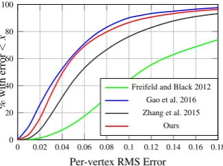
pro-Dataset n/J Offline Online

Fig.5 SCAPE 71 / - 73 m

-TOSCA_Cat 10 / - 66 m

-Fig.8 Dyna_50009 29 / 10 21 m 70 s

Fig.9 SCAPE 70 / 20 72 m 232 s

Fig.10 SCAPE 71 / 20 73 m 919 s

Fig.11 TOSCA_Cat 10 / 5 66 m 154 s Fig.12 Dyna_50009 29 / 10 21 m 100 s Fig.13 Dyna_50021 20 / 10 99 m 321 s

Table 1:Timings obtained with our prototype MATLAB implemen-tation for fixed K=4, but different numbers of training shapes n and principal variations J.

vides a representation of volumetric objects and their deformations which retains physical plausibility. In particular, Fig.13shows that our results are comparable to MoSh [LMB14] which models bones and muscles explicitly. If the training data set contains large bend-ing distortions at joint locations (see e.g. the armpits in Fig.2b), this will be picked up by the first few principal variations since they account for a lot of the variance in the Gram matrix (see Fig.1 and Fig.5). For example, one can see in Fig.10that joints are fairly easy to bend while showing realistic muscle deformation.

In comparison to the original PGA model [FLPJ04], which deals with a low dimensional medial axis description, we consider high dimensional shape manifolds. Furthermore, we extend PGA to the time-discrete setting and introduce a rigid body motion invariant distance measure. This invariance is a substantial advantage over the Shell PCA model [ZHRS15], which is based on vertex displace-ments and hence alignment-dependent. To this end, the Shell PCA model [ZHRS15] only allows for small deformations, i.e. mesh editing and model fitting applications are out of reach of this purely elastic PCA approach.

There are many avenues for future work. It would be interesting to translate the concept of the Mahalanobis distance to our sub-manifold so that we have a notion of the likelihood of a recon-structed shape. Although we have used the space of discrete shells as our motivating example, our proposed time-discrete PGA may have other applications in machine learning with a modified energy functionalWapproximating an alternate measure of squared dis-tance with a potentially different invariance principle. In terms of efficiency, the model reduction technique proposed in [vRESH16] would be ideal for speeding up our method. Since our submanifold works with convex combinations of principal variation shapes, a subspace of deformations trained on samples from the submanifold would dramatically reduce the computational cost and probably al-low for real-time performance.

Acknowledgments

The authors are grateful to Mirela Ben-Chen, Michael Black, Klaus Hildebrandt, Peter Schröder and Max Wardetzky for their detailed and valuable feedback at different stages of this project, as well as to Josua Sassen for proofreading and helping with coding acceler-ations. The data in Fig.10as well as all results shown for compar-ison were kindly provided by Jie Yang. B. Heeren and M. Rumpf

acknowledge support by the FWF in Austria under the grant S117 (NFN) and by the Hausdorff Center.

[image:12.595.63.282.81.184.2]

References

[ACPH06] ALLEN B., CURLESS B., POPOVI ´C Z., HERTZMANN

A.: Learning a correlated model of identity and pose-dependent body shape variation for real-time synthesis. In Proc. ACM SIG-GRAPH/Eurographics Symposium on Computer Animation (2006), pp. 147–156.3

[ASK∗_{05] ANGUELOV D., SRINIVASANP., KOLLERD., THRUN S.,}

[image:12.595.313.558.119.724.2]

RODGERSJ., DAVISJ.: SCAPE: shape completion and animation of people. InACM Trans. Graph.(2005), vol. 24, pp. 408–416.3,6

[BBK08] BRONSTEINA. M., BRONSTEINM. M., KIMMELR.: Numer-ical geometry of non-rigid shapes. Springer Science & Business Media, 2008.6

[BEKB15] BOSCAINID., EYNARDD., KOUROUNISD., BRONSTEIN

M. M.: Shape-from-operator: Recovering shapes from intrinsic opera-tors.Comput. Graph. Forum 34, 2 (2015), 265–274.3

[CLZ13] CHENY., LIUZ., ZHANGZ.: Tensor-based human body mod-eling. InProc. CVPR(2013), pp. 105–112.3

[CSBC∗_{17] CORMANE., SOLOMONJ., BEN-CHENM., GUIBASL.,}

OVSJANIKOVM.: Functional characterization of intrinsic and extrinsic geometry.ACM Trans. Graph. 36, 2 (2017), 14.3

[FB11] FRÖHLICHS., BOTSCHM.: Example-driven deformations based on discrete shells. InComput. Graph. Forum(2011), vol. 30, pp. 2246– 2257.3,8,10

[FB12] FREIFELDO., BLACKM.: Lie bodies: A manifold representation of 3d human shape. InProc. ECCV(2012).3,7,8

[FLPJ04] FLETCHERP. T., LUC., PIZERS. M., JOSHIS.: Principal geodesic analysis for the study of nonlinear statistics of shape. IEEE Trans. Med. Imaging 23, 8 (2004), 995–1005.3,4,11

[GH97] GARLANDM., HECKBERTP. S.: Surface simplification using quadric error metrics. InProc. SIGGRAPH(1997), pp. 209–216.10

[GHDS03] GRINSPUNE., HIRANIA. N., DESBRUNM., SCHRÖDER

P.: Discrete shells. InProc. ACM SIGGRAPH/Eurographics Symposium on Computer Animation(2003), pp. 62–67.2,4

[GLL∗_{16] GAOL., LAIY.-K., LIANGD., CHENS.-Y., XIAS.:}

Ef-ficient and flexible deformation representation for data-driven surface modeling.ACM Trans. Graph. 35, 5 (2016), 158.3,7,8

[HH96] HEAPT., HOGGD.: Extending the point distribution model us-ing polar coordinates.Image Vis. Comput. 14, 8 (1996), 589 – 599.3

[HLRB12] HIRSHBERG D., LOPER M., RACHLIN E., BLACK M.: Coregistration: Simultaneous alignment and modeling of articulated 3d shape. InProc. ECCV(2012), pp. 242–255.3

[HRS∗_{14] HEERENB., RUMPFM., SCHRÖDERP., WARDETZKYM.,}

WIRTHB.: Exploring the geometry of the space of shells. InComput. Graph. Forum(2014), vol. 33, pp. 247–256.3,4

[HRWW12] HEEREN B., RUMPFM., WARDETZKYM., WIRTHB.: Time-discrete geodesics in the space of shells. InComput. Graph. Forum (2012), vol. 31, pp. 1755–1764.3,4

[HSS∗_{09] HASLERN., STOLLC., SUNKELM., ROSENHAHNB., SEI} -DELH.-P.: A statistical model of human pose and body shape. In Com-put. Graph. Forum(2009), vol. 28, pp. 337–346.3

[Ken84] KENDALLD. G.: Shape manifolds, Procrustean metrics, and complex projective spaces. Bull. London Math. Soc. 16, 2 (1984), 81– 121.3

[KMP07] KILIANM., MITRAN. J., POTTMANNH.: Geometric model-ing in shape space. InACM Trans. Graph.(2007), vol. 26, p. 64.3

[LMB14] LOPERM., MAHMOODN., BLACKM. J.: MoSh: Motion and shape capture from sparse markers. ACM Trans. Graph. 33, 6 (2014), 220.9,11

[LMR∗_{15] LOPERM., MAHMOODN., ROMEROJ., PONS-MOLLG.,}

BLACKM. J.: SMPL: A skinned multi-person linear model.ACM Trans. Graph. 34, 6 (2015), 248:1–248:16.3

[MG03] MOHRA., GLEICHERM.: Deformation Sensitive Decimation. Tech. rep., University of Wisconsin, 2003.10

[Pen06] PENNECX.: Intrinsic statistics on Riemannian manifolds: Basic tools for geometric measurements. J. Math. Imaging Vis. 25, 1 (2006), 127–154.3

[PMRMB15] PONS-MOLL G., ROMEROJ., MAHMOOD N., BLACK

M. J.: Dyna: A model of dynamic human shape in motion.ACM Trans. Graph. 34, 4 (2015), 120:1–120:14.1,3

[ROA∗_{13] RUSTAMOVR. M., OVSJANIKOVM., AZENCOTO., BEN}

-CHENM., CHAZALF., GUIBASL.: Map-based exploration of intrinsic shape differences and variability.ACM Trans. Graph. 32, 4 (2013), 72.

3

[RW15] RUMPF M., WIRTH B.: Variational time discretization of geodesic calculus. IMA J. Numer. Anal. 35, 3 (2015), 1011–1046. 4,

5

[SA07] SORKINEO., ALEXAM.: As-rigid-as-possible surface model-ing. InProc. Eurographics Symposium on Geometry Processing(2007), pp. 109–116.2,8

[SC15] SEGUYV., CUTURIM.: Principal geodesic analysis for probabil-ity measures under the optimal transport metric. InAdvances in Neural Information Processing Systems(2015), pp. 3312–3320.3

[SP04] SUMNERR. W., POPOVI ´CJ.: Deformation transfer for triangle meshes.ACM Trans. Graph. 23, 3 (2004), 399–405.3

[SSP07] SUMNERR. W., SCHMIDJ., PAULYM.: Embedded deforma-tion for shape manipuladeforma-tion.ACM Trans. Graph. 26, 3 (2007), 80.8

[SZGP05] SUMNERR. W., ZWICKERM., GOTSMANC., POPOVI ´CJ.: Mesh-based inverse kinematics.ACM Trans. Graph. 24, 3 (2005), 488– 495.3,8

[TPBF87] TERZOPOULOS D., PLATT J., BARR A., FLEISCHER K.: Elastically deformable models. InProc. SIGGRAPH(1987), vol. 21, pp. 205–214.2

[TWC∗_{09] TOURNIER M., WU X., COURTY N., ARNAUD E.,}

REVERETL.: Motion compression using principal geodesics analysis. InComput. Graph. Forum(2009), vol. 28, pp. 355–364.3

[vRESH16] VON RADZIEWSKY P., EISEMANN E., SEIDEL H.-P., HILDEBRANDTK.: Optimized subspaces for deformation-based model-ing and shape interpolation.Computers & Graphics 58(2016), 128–138.

2,11

[vTAMZ18] VONTYCOWICZC., AMBELLANF., MUKHOPADHYAYA., ZACHOWS.: An efficient riemannian statistical shape model using dif-ferential coordinates.Med. Image Anal. 43(2018).3

[vTSSH15] VONTYCOWICZC., SCHULZC., SEIDELH.-P., HILDE

-BRANDT K.: Real-time nonlinear shape interpolation. ACM Trans. Graph. 34, 3 (2015), 34:1–34:10.2