Variational Inference
.
White Rose Research Online URL for this paper:
http://eprints.whiterose.ac.uk/128829/
Version: Accepted Version
Article:
Jacobs, W.R., Baldacchino, T., Dodd, T.J. orcid.org/0000-0001-6820-4526 et al. (1 more
author) (2018) Sparse Bayesian Nonlinear System Identification using Variational
Inference. IEEE Transactions on Automatic Control. ISSN 0018-9286
https://doi.org/10.1109/TAC.2018.2813004
[email protected] https://eprints.whiterose.ac.uk/
Reuse
Unless indicated otherwise, fulltext items are protected by copyright with all rights reserved. The copyright exception in section 29 of the Copyright, Designs and Patents Act 1988 allows the making of a single copy solely for the purpose of non-commercial research or private study within the limits of fair dealing. The publisher or other rights-holder may allow further reproduction and re-use of this version - refer to the White Rose Research Online record for this item. Where records identify the publisher as the copyright holder, users can verify any specific terms of use on the publisher’s website.
Takedown
If you consider content in White Rose Research Online to be in breach of UK law, please notify us by
Sparse Bayesian Nonlinear System Identification
using Variational Inference
William R. Jacobs, Tara Baldacchino, Tony Dodd, and Sean R. Anderson
Abstract—Bayesian nonlinear system identification for one of the major classes of dynamic model, the nonlinear autoregressive with exogenous input (NARX) model, has not been widely studied to date. Markov chain Monte Carlo (MCMC) methods have been developed, which tend to be accurate but can also be slow to con-verge. In this contribution, we present a novel, computationally efficient solution to sparse Bayesian identification of the NARX model using variational inference, which is orders of magnitude faster than MCMC methods. A sparsity-inducing hyper-prior is used to solve the structure detection problem. Key results include: 1. successful demonstration of the method on low signal-to-noise ratio signals (down to 2dB); 2. successful benchmarking in terms of speed and accuracy against a number of other algorithms: Bayesian LASSO, reversible jump MCMC, forward regression orthogonalisation, LASSO and simulation error minimisation with pruning; 3. accurate identification of a real world system, an electroactive polymer; and 4. demonstration for the first time of numerically propagating the estimated nonlinear time-domain model parameter uncertainty into the frequency-domain.
Keywords—Bayesian estimation, variational inference, system identification, NARX model.
I. INTRODUCTION
In nonlinear system identification, a popular model class is the nonlinear autoregressive with exogenous inputs (NARX) model [1], [2]. Reasons for this popularity include the compact-ness of the representation, compared to e.g. Volterra series [3], relative simplicity of estimating parameters due to the linear-in-the-parameters structure [4], and the fact that frequency-domain analysis methods have been developed for the model class, facilitating analysis of nonlinear dynamics [5], [6]. The NARX model is a black-box model, meaning that terms are unknown and must be selected - typically regarded as one of the most challenging problems in nonlinear system identification [7], which is the focus of this paper, in a Bayesian context.
Least-squares and maximum likelihood-type methods have dominated NARX model identification, e.g. by forward re-gression [4], [8], forward-backward pruning methods [9], [10], the expectation-maximisation (EM) algorithm [11] and sparse estimation [12], [13]. Bayesian model identification, on the other hand, is advantageous for a number of reasons: (i) parameter uncertainty is intrinsically described, useful for analysis, simulation and control design [14]; (ii) overfitting is avoided by natural penalisation of overly complex models [15]; (iii) model uncertainty can be accurately quantified even
W. Jacobs, T. Baldacchino, T. Dodd, and S. R. Anderson are with the Department of Automatic Control and Systems Engineering, University of Sheffield, Sheffield, S1 3JD UK, e-mail: [email protected]
for data records with relatively few samples [16]; and (iv) prior information can be incorporated where available [17].
There are a range of methods addressing Bayesian nonlinear system identification, which can be divided by model class, e.g. state-space [18], white-box [19], [20], mixture of experts [21], continuous-time [22], Wiener [23] and NARX models [24]–[26]. Bayesian methods for NARX modelling include nonparametric approaches based on Gaussian process regression [24], [25] and sampling methods based on reversible jump Markov chain Monte Carlo (MCMC) [26]. Although MCMC methods tend to be accurate, they are also computationally intensive and can be prohibitively slow, because they tend to rely on large numbers of samples, and may exhibit slow convergence to a stationary distribution [27].
There is a need, therefore, for a computationally efficient algorithm for Bayesian NARX model identification. To address this challenge, we develop a novel method based on variational Bayesian (VB) inference [28], [29]. The algorithm is both simple to implement and computationally efficient, as it is based on closed form updates of relatively low computational complexity. Model term selection is performed using a sparsity inducing hyper-prior, based on a method known as automatic relevance determination (ARD), which is used to iteratively prune redundant terms from the model [15].
Sparse Bayesian learning algorithms using ARD have been developed for solving regression and classification problems with kernel methods [30]–[32], and have inspired alternatives, e.g. applied to signal denoising [33] and pattern recognition problems with correlated errors [34]. However, ARD, as proposed by [31], is not sufficient to perform the term selection problem in a single step for non-trivial problems. A key novelty here is a new algorithm for term selection of NARX models using sparse variational Bayes (SVB) with ARD, where ARD is iteratively applied to a reducing subset of model terms, retaining the subset identified at each iteration, until there is a single term left in the model.
than forward regression orthogonalisation (FRO) [4], Bayesian LASSO [18], and a Bayesian algorithm based on reversible jump MCMC [26].
Elements of this work have been published in brief confer-ence format [35], and have been extended here in a number of important ways: a more thorough and rigorous theoretical development, expanded benchmarking, and application to real-world data. The real real-world data is obtained from a dielectric elastomer actuator (DEA), which is a type of actuator used in soft robotics [36]–[38]. Furthermore, we demonstrate, for the first time, frequency-domain uncertainty analysis for nonlinear systems by propagation of parameter uncertainty from the identified Bayesian model of the DEA into the frequency-domain, using Monte Carlo sampling and nonlinear output frequency response functions (NOFRFs) [6].
The paper is organized as follows. Section II defines the Bayesian NARX model with associated priors. Section III gives background on variational Bayesian inference. In Section IV-A the parameter estimation algorithm for NARX models is derived using variational inference. In Section V the structure detection algorithm for NARX models is derived using variational inference combined with ARD. In Section VI numerical examples are given, along with benchmark analysis, and finally an application to a real-world system (a set of DEAs) using experimental data. The paper is summarised in Section VII.
II. SYSTEM IDENTIFICATION WITHIN ABAYESIAN
FRAMEWORK A. The NARX model
In this section Bayesian inference of linear-in-the-parameters regression models is introduced in the context of the NARX model. Consider a single-input single-output dynamic system as some non-linear function,f(.), of lagged system inputs,uk,
and outputs,yk, at sample timek,
yk=f(xk) +ek (1)
where xk = yk−1, ..., yk−ny, uk−1, ..., uk−nu
and ek is a
zero-mean Normally distributed white noise process with varianceτ−1.n
u andny are the maximum lags, or dynamic
orders, of the input and output respectively. The non-linear function f(.)can be decomposed into a sum of M weighted basis functions, e.g. by polynomials, radial basis functions, wavelets etc., which is a linear-in-the-parameters model,
f(xk) = M X
m=1
θmφm(xk) (2)
= Φkθ (3)
where
Φk= [φ1(xk), φ2(xk), . . . , φM(xk)], Φk ∈R1×M
θ= [θ1, θ2, . . . , θM]T, θ∈RM×1
andΦk is thek’th row of the matrixΦsuch that
Φ= [ΦT1,ΦT2, . . . ,ΦTN]T, Φ∈RN×M
where N is the number of data points. The term selection problem, addressed in this paper, is the selection of the best choice of basis functions, φm, such that f(·) provides a
parsimonious description of the true system behaviour.
B. Bayesian parameter estimation
Bayes’ rule allows us to infer the posterior distribution of the set of model parameters, denotedΘ, given the observed data sety= [y1, . . . , yN]T, then
p(Θ|y) = p(y|Φ,Θ)p(Θ)
p(y) . (4)
In the above equation the term p(y|Φ,Θ)is referred to as the likelihood function and p(Θ)is the prior distribution of the parameters before observing the data. The denominator, p(y)
is named the marginal likelihood and is given as
p(y) =
Z
p(y|Φ,Θ)p(Θ)dΘ. (5)
in order to normalise the posterior distribution.
The evaluation of (5) can be extremely challenging and necessitates the need for approximation methods in all but the most simple of cases [27]. In this paper (5) will be approximated by the use of variational Bayesian techniques.
C. Likelihood function
The likelihood function for the NARX model given in (1) for y under the assumption of a Normali.i.d.noise sequence is
p(y|Φ,θ, τ) =
N Y
k=1
p(yk|Φk,θ, τ) (6)
=
N Y
k=1
N(yk|Φkθ, τ−1) (7)
= τ 2π
N2
exp −τ
2
N X
k=1
(yk−Φkθ)2 !
(8)
whereN(x|µ, σ)denotes the Normal distribution of the variable xwith mean µand varianceσ.
D. Priors
The likelihood function given by (8) is a member of the exponential family and so the choice of an exponential prior is required for conjugacy [39].
The mean, Φkθ, and precision, τ, of the likelihood are
unknown parameters to be inferred and as such the choice of Normal-Gamma prior distribution is made [40] such that
p(θ, τ|α) = p(θ|τ,α)p(τ) (9) = N(θ|0,(τA)−1)
Gam(τ|a0, b0) (10)
= 2π−M/2|A|1/2 b
a0
0
Γ(a0)
τM/2+a0−1
exp−τ
2(θ
TAθ
+ 2b0)
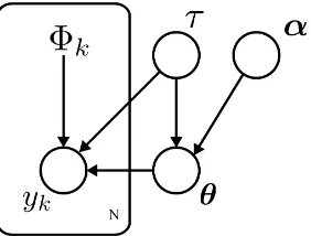
Fig. 1. Probabilistic graphical model of the hierarchical model represented in (14). The plate (box), denoted by the number of data samplesN, indicatesN
i.i.dobservations. The arrows indicate the direction of conditional dependence.
where the Normal distribution has been further parametrised byα= (α1, α2, . . . , αM)T =diag(A). The introduction ofα
into the model naturally incorporates ARD, this is the basis of the sparse estimation framework that will be discussed later. The variableα is an unknown model parameter and will also
be inferred and so requires the introduction of a hyper-prior (prior of a prior),p(α). The choice of a conjugate prior is again
chosen in order to simplify the later analysis. The hyper-prior is therefore assigned as independent Gamma distributions,
p(α) =
M Y
m=1
Gam(αm|c0, d0) (12)
=
M Y
m=1 dc0
0
Γ(c0) αc0−1
m exp(−d0αm) (13)
The model parameters{θ, τ,α}along with hyper-parameters
{a0, b0, c0, d0} can be initialised to have broad/uninformative prior distributions so that the inference process is dominated by the influence of the data [17].
The joint distribution over all of the random variables can now be expressed hierarchically as
p(y,Φ,θ, τ,α) =p(y|Φ,θ, τ)p(θ|τ,α)p(τ)p(α), (14)
assuming τ and α independent and noting that Φ is a function of the observed data and not a random variable. The decomposition can by made more transparent be considering the directed graphical model shown in Figure 1.
E. Prior for Automatic Relevance Determination
ARD has been incorporated into the Bayesian model via the introduction of the hyper-parameter α in (9), where αm
corresponds to the precision (inverse of the variance) of θm. αm therefore controls the magnitude ofθm, ifα−m1= 0then
the precision of θmis infinite and in order to maintain a high
likelihood θm= 0, indicating that them’th model term is not
relevant to the generation of the data. αmis hence acting as
a sparse regularisation term that acts independently on each model weight θm. The values of αm can then be used as a
basis for pruning irrelevant basis functions from the model [41], [42].
In the remainder of this paper the value, α−1
m, is named as
them’th ARD value, where small values indicate terms that are not relevant to the generation of the output. This value will be used to drive the structure detection in the SVB-NARX system identification algorithm introduced in Section V.
F. Posterior distribution
The joint posterior distribution over the model parameters can be found by considering (4), with Θ={θ, τ,α}, where
p(θ, τ,α|y) =p(y|Φ,θ, τ)p(θ|τ,α)p(τ)p(α)
p(y) . (15)
The inclusion of the hyper-parameter,α, into the model causes
the marginal likelihood in the denominator of (15) to become intractable,i.e. no direct analytical solution is possible. Many methods exist for approximating the marginal likelihood [43], commonly these techniques are based on random sampling [27]. Here, variational Bayesian inference will be used because the posterior distribution can be approximated in a series of closed form update equations, avoiding the use of computationally expensive sampling methods.
III. VARIATIONALBAYESIAN INFERENCE
In many non-trivial cases the evaluation of posterior distribu-tions is infeasible as is the case with the linear regression with ARD introduced in the previous section. The full Bayesian treatment in closed form is only feasible for a limited class of models [39]. Numerical integration techniques can always be used, however, the computational expense is often prohibitive. Variational Bayes provides a method for approximating the posterior distribution. In this section some general results of variational Bayesian inference are discussed followed by its application to the linear regression model given by (2).
A. Variational optimisation of the Bayesian model
In the context of Bayesian inference problems variational calculus can be used as a method for approximating posterior distributions. Consider a fully Bayesian model such that all the model parameters are assigned prior distributions as described in Section II. The aim of the inference problem is to find an approximation to the posterior distributionp(Θ|Φ,y)assuming that the marginal distribution,p(y), is intractable. For notational simplicity the conditional dependence on Φwill be assumed implicit and dropped from the following discussion.
The marginal distribution is defined as
p(y) =
Z
Θ
p(y|Θ)p(Θ)dΘ. (16)
lnp(y) = ln
Z
Θ
Q(Θ)p(y|Θ)p(Θ)
Q(Θ) dΘ. (17)
≥
Z
Θ
Q(Θ) lnp(y|Θ)p(Θ)
Q(Θ) dΘ. (18) = L[Q(Θ)] (19)
where (18) follows from Jensen’s inequality [39]. The variational lower bound (VLB)L[Q(Θ)]can be maximised to provide an approximation oflnp(y). Variational optimisation is employed to perform the variational maximization ofL[Q(Θ)]
with respect to the free distributionQ(Θ).
By noting thatQ(Θ)is a proper probability distribution and therefore its integral with respect to Θis equal to unity, and rearranging (18) - (19),
L[Q(Θ)] =
Z
Θ
Q(Θ) lnp(y|Θ)p(Θ)
Q(Θ) dΘ. (20)
=
Z
Θ
Q(Θ) lnp(Θ|y)
Q(Θ) +Q(Θ) lnp(y)dΘ
=
Z
Q(Θ) lnp(y,Θ)dΘ−
Z
Q(Θ) lnQ(Θ)dΘ (21)
lnp(y) = L[Q(Θ)]−
Z
Θ
Q(Θ) lnp(Θ|y)
Q(Θ) dΘ (22) = L[Q(Θ)] +KL(Q(Θ)||p(Θ|y)) (23)
where
KL(Q(Θ)||p(Θ|y)) =−
Z
Θ
Q(Θ) lnp(Θ|y)
Q(Θ) dΘ (24)
is the Kullback-Leibler (KL) divergence from Qtop. A few things of interest can be noted from (22). First, the log marginal distribution, p(y), can be de-constructed into a lower bound on the distribution and a measure of the difference between the true posterior distribution,p(Θ|y), and its approximating distribution, Q(Θ), in the form of the KL divergence. It is then evident that the optimal approximation to the marginal distribution is found by maximising the lower bound, or equivalently minimising the KL divergence. It is also clear that the choice of Q(Θ) =p(Θ|y)would result in an exact match between the bound and the marginal distribution.
B. Factorised distributions
In order to make the variational optimisation of L[Q(Θ)]
feasible, the family of possible distributions, Q(Θ), over which the optimisation is performed, must be restricted. The assumption is made that the variational distribution can be factorised such that
Q(Θ) =Y
j
qj(Θj) (25)
where eachqj(Θj)are independent, an approximation known as
the mean field theory in physics. The function is maximised with
respect to each distribution qj(Θj) separately while holding
all others fixed.
Substituting the factorised distribution (25) into (21) and then separating the i’th distribution over which to perform the optimisation gives
L[Q(Θ))] =
Z Y
j
qj(Θj)
lnp(y,Θ)− X
j
lnqj(Θj)
dΘ
=
Z qi(Θi)
Z
lnp(y,Θ)Y
j6=i
qj(Θj)dΘj
dΘi
−
Z
qi(Θi) lnqi(Θi)dΘi+const (26)
where the terms Q
j6=iqj(Θj) lnqj(Θj) have been absorbed
into a constant term.
In order to find the distribution qi(Θi) that maximises
L[Q(Θ)]a variational optimisation is performed with respect to qi(Θi) such that (full details of the following derivations
can be found in [44])
δL[qi(Θi)] δqi(Θi)
= ∂
∂qi(Θi)
qi(Θi)
Z
lnp(y,Θ)Y
j6=i
qj(Θj)dΘj
−qi(Θi) lnqi(Θi)
(27)
=
Z
lnp(y,Θ)Y
j6=i
qj(Θj)dΘj
−lnqi(Θi) +const. (28)
where δFδf[f((xx))] denotes the functional derivative of the func-tional F[f(x)] with respect to the function f(x) and ∂f∂x(x) denotes the partial derivative of the function f(x)with respect to the variable x.
The integral that forms the first term on the right hand side of (28) is the expectation of the log joint distribution where the expectation is taken with respect to all of the distributions qj(Θj)for which j6=i, such that
Ej6=i[ln(y,Θ)] = Z
lnp(y,Θ)Y
j6=i
qj(Θj)dΘj (29)
where Ej6=i denotes the expectation with respect to the
distributions q over all the variables in the set Θ for which j 6=i.
Substituting (29) into (28), equating to zero and rearranging for the variational distribution, a general expression for the optimal solution and therefore the update of the ith factor of the variational distribution qi(t+1)(Θi)is then given by
Performing the update (30) for each factor qj(Θj) of the
variational distribution completes one optimisation step of
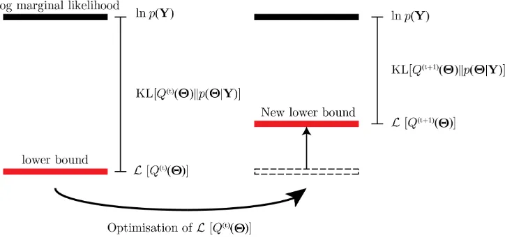
L[Q(Θ)]. The optimisation is performed iteratively where t indicates the current iteration such that q(jt+1) is the update using the statistics of the distributions q(jt) at the previous
iteration, see Figure 2.
Equation (30) can also be arrived at using the Kullback-Leibler divergence, as detailed in [39] in Section 10.1.1.
C. Convergence
The lower bound is guaranteed to converge because it is convex with respect to each of the factors of q(it+1)(Θi). In
order to facilitate the computation of the VLB, (21) can be written more explicitly as
L[Q(Θ)] =EΘ[lnp(y,Θ)]−EΘ[lnQ(Θ)] (31) which is the form used to monitor convergence of the algorithm. Although the calculation of the VLB is not required for the inference problem it provides a check that the algorithm, as well as the theory behind it, is functioning correctly as the bound is guaranteed to increase with each update of the variational distribution [44]. In addition, it is important to note that the VLB will be used later as a method for model comparison and therefore must be calculated for that purpose.
IV. VARIATIONAL INFERENCE FORNARXMODELS
A. Variational inference of model parameters
The variational Bayesian inference procedure can now be applied to the NARX model defined by (2) following [45]. Applying the approximation defined by (25), the assumption is made that the posterior distribution p(θ, τ,α|y) can be approximated by
Q(θ, τ,α) =q(θ, τ)q(α) (32)
whereby the VLB can be maximised with respect to each factor. From (18), the VLB is given by
L[Q(θ, τ,α)] =
Z Z Z
Q(θ, τ,α) (33)
lnp(y|Φ,θ, τ, α)p(θ, τ|α)p(α)
Q(θ, τ,α) dθdτdα.
Using the results of the variational Bayesian inference derived above, the optimisation of the bound is performed via (30) for the distributions q(θ, τ)andq(α)resulting in a set of closed
form update equations.
1) Update forq(θ, τ): The variational posterior qK(θ, τ)is
found by maximising the VLB,L(Q), with fixed q(α), where
the subscriptK denotes the updated parameters. Noting that p(y,Θ)is given by (14) whenΘ={θ, τ,α}, then from (30)
the update equation forq(θ, τ)is given as
lnqK(θ, τ) = lnp(y|Φ,θ, τ) +Eα[lnp(θ, τ|α)]
+const (34)
=
M
2 +a0−1 +
N
2
ln(τ)
−τ
2 θ
T
Eα[A] +
N X
k=1
ΦTkΦk ! θ + N X k=1 y2k−2
N X
k=1
ykΦkθ+ 2b0
!
+const (35)
where p(y|Φ,θ, τ) and p(θ, τ|α) are given by (8) and (11)
respectively and all the terms not dependent on θ andτ have
been absorbed into the constant term.
Given that the likelihood function, (8), is in the form of a Normal distribution, the conjugate Normal-Gamma prior, (11), is chosen. Hence, the posterior distribution can be expressed as
qK(θ, τ) =N(θ|θK, τ−1VK)Gam(τ|aK, bK), (36)
The method of completing the square is used to find the exponent of the Normal distribution in the posterior by equating coefficients of (35) and (36). First, separating out all the coefficients of −τ
2θ
Tθ
, to findVK−1
−τ
2θ
T
V−K1θ = −τ
2θ
T N X
k=1
ΦTkΦk+Eα[A]
!
θ(37)
V−K1 =
N X
k=1
ΦTkΦk+Eα[A]. (38) Separating out the coefficients of θ to findθK
τθTV−K1θK = τθT
N X
k=1
ΦTkyk (39)
θK = VK
N X
k=1
ΦT
kyk. (40)
Now, (36) can be expressed as
lnqK(θ, τ) = lnN(θ|θK, τ−1VK)
−τ
2
N X
k=1
y2k+ 2b0−θTKV−K1θK !
+
a0−1 + N
2
ln(τ) +const. (41)
where the second and third terms in (41) are to be equated with the terms in the Gamma distribution. Equating coefficients of τ
−τ bK = − τ
2
N X
k=1
yk2+ 2b0−θTKVK−1θK !
(42)
bK = b0+
1 2 N X k=1 y2
k−θTKVK−1θK !
Fig. 2. Variational inference is performed by iteratively updating the VLB via an optimisation step: the diagram illustrates the variational Bayesian update according to (30).
And finally equating coefficients oflnτ
(aK−1) lnτ =
a0−1 + N
2
lnτ (44)
aK = a0+ N
2 . (45)
The update oflnq(θ, τ)is by the computation of (38), (40),
(43) and (45).
2) Update for qK(α): The variational posterior q(α) is
found by maximising the VLB,L(Q), with fixedq(θ, τ). Using
(30), and equating coefficients ofαm,
lnqK(α) = Eθ,τ(lnp(θ, τ|α)) + lnp(α) +const
=
M X
m=1
lnGam(αm|cK, dKm) (46)
where
cK = c0+
1
2 (47)
dKm = d0+ 1 2Eθ,τ[τ θ
2
m]. (48)
The update ofq(α)is hence performed by the computation of
(47) - (48).
The required expectations are found by considering the standard moments of the relevant distributions [39] such that
Eθ,τ[τ θ2m] =θ2K
m
aK bK
+VKmm (49)
and the required expectation for the update of q(θ, τ)is given
by
Eα[A] =AK (50) whereAK is a diagonal matrix with elements
Eα[αm] = cK dKm
. (51)
The variational approximation, Q(θ, τ,α) = q(θ, τ)q(α),
to the true posterior p(θ, τ,α|y)is found by updatingq(θ, τ)
and q(α)by iterating between the update equations defined
by (38), (40), (43) and (45), and (47)-(48) respectively. These updates then form an iterative algorithm that is summarised in Algorithm 1. The variables bK, dKm,θK andVK must first
be initialised: bK and dKm are initialised to their respective
prior values, bK|t=0=b0 anddK|t=0=d0.θK andVK are
initialised using the least squares estimate, such that
θK|t=0 = (ΦTΦ)−1ΦTy,
(52)
VK|t=0 = ΦTΦ. (53)
B. Variational lower bound L(Q)
The VLB is found by considering (31). The dependencies between the parameters in the first term in (31) are easily determined by considering the joint distribution given by (14) and the probabilistic graphical model in Figure 1. Expanding the second term follows from (32) along with (36) and (46). The lower bound is then given by
L[Q(Θ)] =EΘ[lnp(y,Θ)]−EΘ[lnQ(Θ)] (54) =Eθ,τ[ln(p(y|Φ,θ, τ))] +Eθ,τ,α[lnp(θ, τ|α)]
+Eα[lnp(α)]−Eθ,τ[lnq(θ, τ)]−Eα[lnq(α)]. (55) Taking the expectations of Equations (8), (11), (13), (36) and (46), the components of (55) are evaluated as:
Eθ,τlnp(y|Φ,θ, τ) = N
2(ψ(aK)−lnbK−ln 2π)
−1
2
N X
k=1
a K bK
(yk−Φkθ)2 + ΦkVKΦTk
whereψ(·)is the digamma function.
Eθ,τ,αlnp(θ, τ|α) = M
2 (ψ(aK)−lnbK+ψ(cK)−ln 2π)
−b0 aK bK
−1
2
M X
m=1
lndKm+
cK dKm
a K bK
θ2Km+VKmm
−ln Γ(a0) +a0ln(b0) + (a0−1)(ψ(aK)−lnbK) (57)
Eαlnp(α) =−M(ln Γ(c0) +c0lnd0)
+
M X
m=1
(c0−1)(ψ(cK)−lndKm)−d0
cK dKm
(58)
Eθ,τlnqK(θ, τ) = M
2 (ψ(aK)−lnbK−ln 2π−1)
−1
2ln|VK| −ln Γ(aK) +aKlnbK + (aK−1)(ψ(aK)−lnbK)−aK (59)
EαlnqK(α) =
M X
m=1
((cK−1)ψ(cK) + lndKm)
−M(ln Γ(cK) +cK). (60)
Substituting (56) - (60) into (55) provides an expression for the variational bound as
L(Q) =−N
2 ln 2π+ 1
2ln|VK| −b0
aK bK
−1
2
N X
k=1
a K bK
(yk−ΦkθK)2+ ΦkVKΦTk
+ ln Γ(aK)−aKlnbK+aK
−ln Γ(a0) +a0lnb0−
M X
m=1
(cKlndKm)
+M
1
2 −ln Γ(c0) +c0lnd0+ ln Γ(cK)
(61)
The variational posterior distribution Q(θ, τ,α) can now
be calculated iteratively by computing q(θ, τ) and q(α). At
each iteration the VLB, L(Q)can be computed via (61). The best approximation is found whenL(Q)plateaus such that the condition L(Q)t− L(Q)t−1 <=TL(Q) is met, whereTL(Q) is a predefined threshold.
C. Predictive distribution
Predictions of a new, unseen, data point can be made by calculating a predictive distribution for the model at sample k+ 1. Given the input-output training data D, the task is the evaluation of the distribution p(yk+1|D). The predictive distribution is found by marginalising over the parameters such
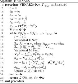
Algorithm 1: VBNARX
1: procedure VBNARX(Φ,y, TL(Q), a0, b0, c0, d0)
2: t= 0 3: bK=b0
4: dK =d0
5: aK =a0+N2
6: cK=c0+12
7: θK = (ΦTΦ)−1ΦTy
8: VK =ΦTΦ
9: while L(Q)t− L(Q)t−1> TL(Q) do
10: t=t+ 1
11: Variational E Step:
12: Eα[A] =AK, where AK,ii=cK/dKi
13: Eθ,τ[τ θ2m] =θK2m
aK
bK +VKmm 14: Variational M Step:
15: V−K1=PNk=1ΦT
kΦk+Eα[A]
16: θK=VKPNk=1ΦTkyk
17: bK =b0+12
PN
k=1yk2−θ T
KV−K1θK
18: dKm=d0+
1
2Eθ,τ[τ θ2m]
19: UpdateL(Q)tvia (61)
20: end while
21: return L(Q)t, cK, dK,ΘK
[image:8.612.320.571.54.322.2]22: end procedure
Fig. 3. Algorithmic description of the parameter estimation procedure for the NARX model using variational Bayesian inference, termed VBNARX
that
p(yk+1|Φk+1,D)
=
Z Z Z
p(Φk+1|Φk+1,θ, τ)p(θ, τ,α|D)dθdτdα
≈
Z Z Z
p(yk+1|Φk+1,θ, τ)q(θ, τ)q(α)dθdτdα
=
Z Z
N(yk+1|Φk+1θK, τ−1)N(θ|θK, τ−1VK)
Gam(τ|aK, bK)dθdτ
=
Z
N(yk+1|Φk+1θK, τ−1(1 + Φk+1VKΦTk+1))
Gam(τ|aK, bK)dτ
=St(yk+1|µ, λ, ν) (62)
where µ = Φk+1θK, λ = baKK(1 + Φk+1VKΦTk+1)−1 and ν = 2aK. The resulting distribution, denoted St, is a Student’s
t-distribution. The distribution overα does not appear in the
third line of the above derivation because it is independent of the other distributions and hence it integrates to unity. In the final step, standard results from convolving conjugate distributions have been used [39]. The mean and variance of the distribution are given by
E[yk+1] = ΦkθK, (63)
Var[yk+1] = (1 + ΦkVKΦTk) bK
(aK−1)
V. STRUCTURE DETECTION FORNARXMODELS WITH VARIATIONAL INFERENCE ANDARD
The variational Bayesian inference procedure provides a method for estimating the posterior distributions of linear in the parameters models, such as those of the NARX form. Through the incorporation of ARD into the procedure, a measure of how relevant each basis function is to the prediction of the data is achieved. Importantly the VLB provides a measure of how good the approximate posterior distribution of the parameters is to the true posterior distribution. For a given data set, the VLB is directly comparable across different models, and hence provides a method for model selection. In this section we take advantage of these features of the variational Bayesian inference in order to develop an algorithm, named the SVB-NARX algorithm, for parsimonious model structure detection.
A. The SVB-NARX algorithm
In overview, the algorithm proceeds by iteratively pruning basis functions from an initial superset of basis function, denotedM0, until there is a single basis function remaining. At each iteration of the algorithm, a subset of the basis functions that are selected at the previous iteration is chosen. The subset selection is performed by making use of the sparse variational inference procedure, defined in Algorithm 1. The variational inference provides a measure of how relevant each basis function is to the generation of the data. The least relevant terms are not included in the new set. The SVB-NARX algorithm is summarised in Algorithm 2,
The initial superset of basis function, M0 is defined as
M0={φm}Mm=1, (65)
whereφmis them’th basis function, corresponding to them’th
column of Φ, and M =|M0| is the total number of basis functions in the current model structure.
At each iteration of the algorithm, denoted by s, the variational Bayesian inference procedure is applied to the model defined by the current set of basis functions,Ms, using
Algorithm 1. Upon convergence of Algorithm 1 the VLB is recorded asL(Q)s, which provides a measure of quality of the
model structure defined by Ms
ARD values, defined in Section II-E, associated with each basis function are calculated as
ARDs=
Eα[αm]−1 M
m=1 (66)
whereEα[αm] is given by equation (51).
Terms that correspond to ARD values falling below the threshold Ts
ARD are pruned from the model,i.e.they are not
included in the new model structure, Ms+1. The threshold is
updated at each algorithm iteration as
lnTARDs = min(lnARDs)
+ max(lnARD
s)−min(lnARDs)
r (67)
with the resolution,r, being a tuning parameter of the algorithm set by the modeller. Consequences of the choice of r are discussed in the following section.
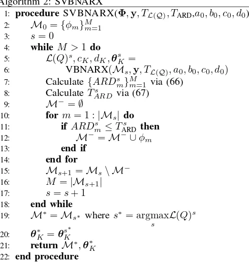
Algorithm 2: SVBNARX
1: procedure SVBNARX(Φ,y, TL(Q), TARD,a0, b0, c0, d0)
2: M0={φm}Mm=1
3: s= 0
4: while M >1do
5: L(Q)s, cK, dK,θsK =
6: VBNARX(Ms,y, TL(Q), a0, b0, c0, d0)
7: Calculate{ARDs
m}Mm=1 via (66)
8: CalculateTs
ARD via (67)
9: M−=∅
10: form= 1 :|Ms| do
11: if ARDs
m≤TARDs then 12: M−=M−∪φm
13: end if
14: end for
15: Ms+1=Ms\ M−
16: M =|Ms+1|
17: s=s+ 1 18: end while
19: M∗=Ms∗ wheres∗= argmax
s
L(Q)s
20: θ∗K =θsK∗ 21: return M∗,θ∗
K
[image:9.612.321.566.56.315.2]22: end procedure
Fig. 4. Sparse Bayesian identification of the NARX model using variational inference and automatic relevance determination
The threshold is dependent on the range of the ln(ARD)
values and removes terms at the lower fraction of this range depending on the value of r. This choice of threshold has the advantage of removing increasingly less terms at each algorithm iteration and hence discriminating more in the pruning as the number of basis functions decreases. ln(ARD)values are used to calculate the threshold, because the ARD values associated with highly relevant model terms can be very high in comparison to less relevant (but still correct) model terms.
ln(ARD)values will provide greater discrimination between less relevant terms in this case. The iteration ends whenM = 1
(all but one term have been pruned from the model).
The result of the iterative pruning is a selection of models,
Ms with a diminishing number of basis functions, each of
which can directly be compared by its associated VLB,L(Q)s.
The optimal model choice,M∗, is then selected as the model
with the greatest maximum lower bound such that
M∗=Ms∗, where s∗=max
s L(Q) s.
(68)
B. Algorithm Initialisation and Choice of Hyper-parameters
The SVB-NARX algorithm requires initialisation of the hyper-parameters associated with the prior distributions, namely a0, b0, c0 and d0. A standard choice of hyper-parameters are a0=c0= 1×10⁻²andb0=d0= 1×10⁻⁴, so as to produce uninformative prior distributions [39], [45]. The mean of the Gamma distribution on τ−1 at these values is undefined but it has mode b0/(a0+ 1)≈ 1×10⁻⁴. This implies that the most likely variance onθ will be smalla priori. Thea priori
variance on τ−1 is also undefined at these values, however the variance on τ can be computed as a0/b20 = 1×10⁶. It can hence be concluded that although the prior distribution indicates a preference forθto take small values, this effect will
be minimal on the inference because of the broad distribution. The same reasoning can be applied to the prior distribution on
α.
The single tuning parameter of the algorithm is the resolution, r, whose value is set in advance by the modeller. It is named resolution because it defines the region of ARD values that are pruned from the model via (67). Increasing the value ofrleads to a higher resolution, resulting in less terms being pruned at each iteration, s, and consequently longer computation time. Conversely, reducing the value of r increases the number of terms pruned at each iteration.
It is to be noted that if r is chosen too small then correct model terms may be incorrectly pruned from the model. However, the value of r can always be set high to avoid incorrectly pruning terms, where the only penalty is longer computation time. In addition, to mitigate effects introduced by tuning rit should also be noted that for a given model and data set the VLB is independent of the resolution that produced it. This allows for multiple algorithm runs with varying values of r to produce models that are directly comparable.
C. Algorithm properties
In this section we explain key properties of the algorithm.
1) Model selection by the variational lower bound: In the previous section it is stated that the optimal model choice is taken to be the model that maximises the VLB after it has reached convergence.
In (4) the conditional dependencies on the model Ms are
neglected. Explicitly including the conditional dependencies, (4) can be written
p(Θ|Φ,Ms) =
p(y|Φ,Θ,Ms)p(Θ|Ms) p(y|Ms)
(69)
Considering the posterior distribution over the models,Ms,
conditional on the data and applying Bayes’ theorem the posterior distribution over thes’th model is given by
p(Ms|y) = p(
y|Ms)p(Ms)
p(y) . (70)
The first term in the numerator on the right hand side of (70) is the same as the marginal likelihood in (69). Setting equal prior distributions p(Ms)for each model and noting that the
denominator is constant for a given data set, the posterior is proportional to the marginal likelihood in (69)
p(Ms|y) ∝p(y|Ms). (71)
For a more in depth discussion of the role of the marginal likelihood in Bayesian model selection see [15].
The VLB, L(Q)s, calculated for each model is an
approx-imation of the marginal likelihood, p(y|Ms). Equation (71)
therefore provides the justification for using the VLB as a criterion for selecting the final model structure.
2) Computational complexity: The computational complexity of the SVB-NARX algorithm is dominated by the matrix inversion of the result of (38) in order to perform the variational update of the model parameters. The computational complexity of the algorithm is therefore cubic in the number of parameters O(M3). The pruning step of the algorithm results in a smaller set of model parameters, M, being evaluated at each iteration of the algorithm and hence the time taken for the variational updates to reach convergence decreases significantly as the algorithm progresses.
In practice the computational complexity of SVB-NARX translates to run times that can be an order of magnitude less than methods based on MCMC (see Section VI). The long computation times in MCMC methods are not attributed to the complexity of individual mathematical operations, but rather tends to depend on the random initialisation of samples, and whether the initialisation is close to the stationary distribution of model and parameters, and is then affected by how long the Markov chain takes to converge to that stationary distribution: these aspects are difficult to quantify precisely because they depend on the inherent randomness of the MCMC process. Similar computational comparisons have been made elsewhere in the literature for VB and MCMC methods [46].
VI. RESULTS ANDDISCUSSION
In this section the SVB-NARX algorithm is demonstrated and benchmarked on a numerical example and then applied to a real system. The benchmark algorithms include a sparse Bayesian LASSO (BL) algorithm [18], a Bayesian algorithm by some of the authors based on reversible jump MCMC (RJMCMC) [26], the FRO algorithm based on orthogonal least squares [4], a standard LASSO algorithm [47], and a simulation based method, SEMP, [9]. The algorithm is then applied to the identification of a real system, a dielectric elastomer actuator used in soft robotics [36], [48], [49].
A. Benchmarking on a known nonlinear system
The SVB-NARX algorithm was demonstrated and bench-marked on the system below, a polynomial NARX model, which has previously been used as a challenging example because a popular algorithm, FRO, fails to select all terms correctly [9], [50],
yk=θ1yk−2+θ2yk−1uk−1+θ3u2k−2
where θ1 =−0.5,θ2 = 0.7,θ3= 0.6, θ4= 0.2, θ5=−0.7, andek is a Normally distributed white noise sequence drawn
from the distribution N(ek|0, σe2). The system was simulated
for N = 1000 data samples at a noise level ofσ2
e = 0.0004
generating signals with a signal-to-noise ratio (SNR) ≈20 dB, where SNR=10 log10 σy2/σ2e
, whereσ2
y is the noise-free
output variance. Additional SNRs in the range 2-20 dB were also investigated). The input, uk, was drawn from a uniform
distribution in the range [−1,1].
To perform the term selection, a superset of basis functions is typically defined. For polynomial models, basis functions in the superset can take the form of any polynomial combination of the elements of xk up to a maximum ordernp [2]. In this
case np = 3. In addition the maximum dynamic orders for
input and output were set to nu = ny = 4. This led to an
initial superset of M= 164 model terms (for all algorithms). Algorithm initialisation was performed as follows.
SVB-NARX: for SVB-NARX initialisation, prior distibutions were set using hyper-parameter values as discussed in Section V-B. The resolution of the algorithm was tested at values of r = 10,100 and 1000 to illustrate the effect of this tuning parameter.
Bayesian-LASSO: the BL algorithm requires the manual tuning of the parameter λBL, which is defined as the variance
of the noise, σ2
e. Setting λBL to the true noise variance was
found to result in an incorrect term selection. The parameter was therefore set to λBL = 0.002, which gave the correct
terms.
RJMCMC: the RJMCMC algorithm hyper-parameters for prior distributions were set as in [26]. In addition the noise variance was manually set to σ2
e = 0.1. The RJMCMC
algorithm was executed 100 times for 100,000 iterations per execution.
FRO: for FRO, the algorithm is usually terminated when the error reduction (ERR) ratio value drops below a threshold: in this case the threshold was set to 0.01.
LASSO: the LASSO algorithm used here was based on the method reported in [47], with regularisation weight set to λLASSO= 0.0043, selected from a range of values to minimise
the mean squared prediction error (MSPE) from a 10-fold cross-validation test, where MSPE= 1
N P
k(yk −yˆmpo,k)2, where
ˆ
ympo,k is the k’th element of the model predicted output.
SEMP: the SEMP algorithm is usually terminated when the change in MSPE drops below a threshold, where a decrease of less than 1×10⁻⁶ was taken as the threshold here.
All algorithms were implemented by the authors in Matlab except BL, where a toolbox by the original authors of [18] at https://github.com/panweihit/BSID was used.
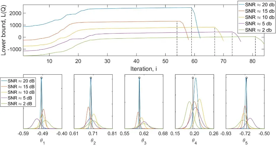
[image:11.612.332.560.76.496.2]The SVB-NARX algorithm, with r= 100, performed well over a range of noise levels, selecting the correct model terms at SNRs of 2-20 dB (see Figure 5, where the dashed black line indicates the correct model structure and corresponds in all instances to the maximum of the variational bound). The true model parameters were within the 95% confidence intervals at all noise levels (this is not shown in Figure 5 in order not to overcrowd the plots on the bottom row). As should be expected, the variance of the parameter distributions increases with increasing noise, see Figure 5.
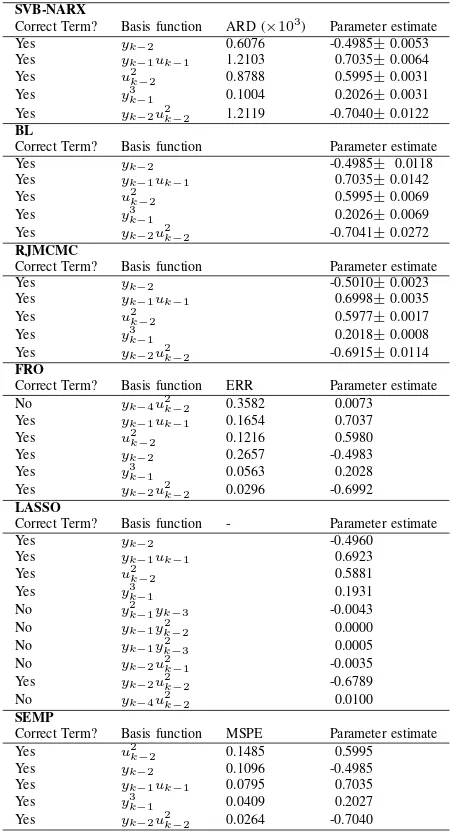
TABLE I. COMPARISON OF TERM SELECTION AND PARAMETER ESTIMATION FOR THE SYSTEM GIVEN BY(72).
SVB-NARX
Correct Term? Basis function ARD (×103
) Parameter estimate Yes yk−2 0.6076 -0.4985±0.0053
Yes yk−1uk−1 1.2103 0.7035±0.0064
Yes u2
k−2 0.8788 0.5995±0.0031
Yes y3
k−1 0.1004 0.2026±0.0031
Yes yk−2u 2
k−2 1.2119 -0.7040±0.0122 BL
Correct Term? Basis function Parameter estimate
Yes yk−2 -0.4985± 0.0118
Yes yk−1uk−1 0.7035±0.0142
Yes u2
k−2 0.5995±0.0069
Yes y3
k−1 0.2026±0.0069
Yes yk−2u 2
k−2 -0.7041±0.0272 RJMCMC
Correct Term? Basis function Parameter estimate
Yes yk−2 -0.5010±0.0023
Yes yk−1uk−1 0.6998±0.0035
Yes u2
k−2 0.5977±0.0017
Yes y3
k−1 0.2018±0.0008
Yes yk−2u 2
k−2 -0.6915±0.0114 FRO
Correct Term? Basis function ERR Parameter estimate No yk−4u
2
k−2 0.3582 0.0073
Yes yk−1uk−1 0.1654 0.7037
Yes u2
k−2 0.1216 0.5980
Yes yk−2 0.2657 -0.4983
Yes y3
k−1 0.0563 0.2028
Yes yk−2u 2
k−2 0.0296 -0.6992 LASSO
Correct Term? Basis function - Parameter estimate
Yes yk−2 -0.4960
Yes yk−1uk−1 0.6923
Yes u2
k−2 0.5881
Yes y3
k−1 0.1931
No y2
k−1yk−3 -0.0043
No yk−1y 2
k−2 0.0000
No yk−1y 2
k−3 0.0005
No yk−2u 2
k−1 -0.0035
Yes yk−2u 2
k−2 -0.6789
No yk−4u 2
k−2 0.0100
SEMP
Correct Term? Basis function MSPE Parameter estimate
Yes u2
k−2 0.1485 0.5995
Yes yk−2 0.1096 -0.4985
Yes yk−1uk−1 0.0795 0.7035
Yes y3
k−1 0.0409 0.2027
Yes yk−2u 2
k−2 0.0264 -0.7040
Fig. 5. Results of Numerical example 1.Top: SVB-NARX model structure detection at varying signal-to-noise ratios (SNRs), 2-20dB. The VLB is plotted against algorithm iteration number for each noise level. The correct model structure is indicated by the black dotted line and corresponds to the maximum of the VLB for all noise levels, indicating the correct model structure at all SNRs. The bound converges to a smaller value with increasing noise.Bottom: Parameter distributions calculated at different noise levels. The true parameter is given by the stem plot. As expected the parameter estimates are less certain at higher noise levels.
Fig. 6. Comparison of benchmark algorithms at varying levels of SNR using the average root normalised mean square error (RNMSE) of identified model parameters. The RNMSE average was taken over 100 Monte Carlo simulations. Error bars show 2 standard deviations from the mean.
[13] (the true model structure was not recovered at any value of λLASSO). Finally, the SEMP algorithm correctly identified
the model structure.
[image:12.612.62.291.370.512.2]The same model was used to investigate the effect of noise on the identification performance for each of the benchmark algorithms (RJMCMC was omitted because of the long compu-tation time required). In total, 100 input-output data sets were generated for six different SNR values in the range 2-20 dB. The initial super-set of model terms was set as described above (164 terms). The root of the normalised mean squared error
Fig. 7. Average timings of structure detection algorithms over 10 runs. Error bars show 2 standard deviations from the mean.
(RNMSE) of the model parameters was used as a performance index, defined askˆθ−θk2/kθk2, whereθˆ was the estimate of
the true parameter θ. Note that the parameters of incorrectly
[image:12.612.331.563.372.513.2]To investigate computational efficiency, the benchmark example was repeated varying the size of the initial superset of model terms. This was done by increasing the dynamic orders ny=nu= 2, . . . ,8. RJMCMC was omitted because it
took orders of magnitude longer than the other algorithms (for 164 terms, it took ∼20 seconds per trial of 100,000 iterations but requiring multiple trials, in this case 100, i.e.
∼2000 seconds). The SVB-NARX algorithm was run at two resolution levels of r= 10 andr = 100 to demonstrate the effect of this tuning parameter. Initialisation and term selection for all other algorithms remained the same. Computational times were averaged over 10 trials. For a small initial basis function set (<100 terms) all of the tested algorithms were comparable, taking under 10 seconds to complete (Figure 7). Greater differences between algorithms were seen for more model terms: in particular SVB-NARX was fastest for over 500 terms and had a relatively flat trend as the number of terms increased toward 1000 (Figure 7). The greater efficiency of SVB-NARX is due to the pruning procedure removing multiple terms at each iteration, which rapidly decreases the dimensionality of the inference task as the algorithm progresses, leading to significantly decreased computation time at each iteration.
In summary, the benchmark has demonstrated that SVB-NARX has advantages in the automated tuning of the noise variance, as well as increased computational efficiency for large numbers of terms. The automated tuning of the noise variance with SVB-NARX is particularly important because alternatives such as BL and RJMCMC do not select the correct terms for certain manually tuned values of noise variance, and the successful value would be unknown for real world problems.
B. Experimental system identification of a dielectric elastomer actuator
The SVB-NARX algorithm was applied in this section to the identification of a set of six dielectric elastomer actuators (DEAs), which are a type of soft-smart actuator used in robotics [36], [48], [49]. DEAs are known to exhibit nonlinear dynamics, posing challenges for control design [37], [38], [52].
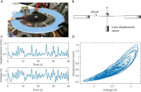
The dataset used in this investigation has already been published and so we only give brief details here, readers are referred to [37] for more information. The input-output data comprised voltage as input, and displacement as output (see Figure 8). The voltage input signal was designed as band-limited white noise (0-1Hz), with amplitude offset to lie in the range 1.5-3.5V, sampled at 50Hz (and then down-sampled for identification to 12.5Hz). We used 160 seconds of data for identification, N=2000 samples, and partitioned the data for identification and validation (comprising N=1000 data samples for each segment). Detailed results are given for one DEA, and then summarised for the remaining five. For comparison, the SEMP, FRO and BL algorithms are also evaluated.
Regarding initialisation of the identification algorithms, the superset of initial model terms was generated withnu=ny = 3
[image:13.612.328.563.93.428.2]and np= 3. The SVB-NARX algorithm was initialised with r= 1000, and hyper-parameters were initialised as in Section V-B. The FRO algorithm was terminated when the ERR value
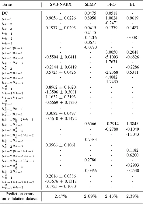
TABLE II. MODEL TERMS AND PARAMETERS OF ADEAIDENTIFIED USINGSVB-NARX, SEMP, FROANDBL. PARAMETER VALUES FOR THE
SVB-NARXIDENTIFIED MODEL ARE GIVEN WITH THEIR95%CONFIDENCE INTERVALS.
Terms SVB-NARX SEMP FRO BL
DC - 0.0475 0.0518
-yk−1 0.9056±0.0226 0.8950 1.0024 0.9619
yk−2 - - -0.2471
-yk−3 0.1977±0.0293 0.0415 0.1379 0.1487
uk−1 - 0.4115 -
-uk−2 - -0.4216 - -0.0081
uk−3 - 0.0671 -
-yk−1yk−2 - -0.0770 -
-yk−1uk−1 - - 3.0050 0.2048
yk−1uk−2 -0.5504±0.0411 - -5.1093 -0.6826
yk−1uk−3 - - 1.7671
-y2
k−2 -0.2144±0.0419 - - -0.2286
yk−2uk−1 0.5725±0.0426 - -2.2368 0.5311
yk−2uk−2 - - 4.4082
-yk−2uk−3 - - -1.7435
-u2
k−1 0.8962±0.1620 - -
-uk−1uk−2 -1.3596±0.3081 - -
-uk−2uk−3 1.1632±0.3193 - -
-u2
k−3 -0.6669±0.1730 - -
-y2
k−1yk−2 - - -
-y2
k−1uk−1 0.3082±0.0497 - -
-yk−1yk−2uk−3 -0.5610±0.1472 - -
-yk−1u 2
k−1 - 0.6566 - 0.2914 1.3845
yk−1u 2
k−3 - - -0.2780 -0.1049
yk−1uk−1uk−2 - - - -1.3043
yk−1u 2
k−2 - -0.7383 -
-y2
k−2uk−3 0.3906±0.1061 -
-yk−2yk−3uk−2 - - - 0.1182
yk−2uk−2uk−3 - - - 0.6200
yk−2uk−1uk−3 - 0.2786 -
-yk−2u 2
k−3 - - - -0.2903
yk−3u 2
k−1 - -0.0366 - -0.2530
u3
k−1 0.2016±0.0386 - -
-uk−1uk−2uk−3 -0.3676±0.1317 - -
-u2
k−2uk−3 0.1755±0.1030 - -
-Prediction errors
on validation dataset 2.47% 2.09% 2.43% 2.39%
fell below 1×10⁻⁵. The SEMP algorithm was terminated by thresholding the MSPE. The BL algorithm required the selection of the tuning parameter λ, which was set toλ= 5.5×10⁻⁴, selected by running the algorithm over a range of values of λand selecting the model with the minimum prediction error over the training data.
Fig. 8. Experimental setup for the dielectric elastomer actuators (DEAs). A: Photo of the DEA experimental rig: An elastomer film is anchored over a rigid blue plastic frame. Electrodes are painted on with conducting carbon grease (inner black circle), to form the DEA, and connected to an external power supply. A metal ball weights the DEA in the centre. On application of a voltage across the DEA the actuator expands raising the ball in the vertical direction: the resulting vertical displacement is the output measured by a laser displacement sensor underneath. B: Diagram of the DEA experimental rig. C: Typical input (voltage) and output (displacement) data obtained from one DEA experiment (zoomed for clarity to the first 40 seconds). D: Input vs output (voltage-displacement) plot, indicating nonlinear dynamics of the actuator.
A striking feature of the identified NARX models, shown in Table II, is that they consist of different terms, implying that they might describe different dynamics. However, comparison of dynamics based on the model equation is not informative because they are not necessarily unique descriptors [2]. NARX models are preferably compared and analysed in the frequency domain, where the dynamics should be uniquely described [2]. We performed such an analysis here via nonlinear output frequency response functions (NOFRFs) [2], [6].
We briefly explain the NOFRF analysis procedure here. The frequency response of a nonlinear system, Y(jω), can be analysed using the sum of n-th order output spectra, Y(jω) = P
nYn(jω) [53], which is based on the standard
description originating in Volterra series analysis of nonlinear systems,y(t) =P
nyn(t), whereyn(t)is known as then-th
order system output [54]. The NOFRFs allow the reconstruction of then-th order output spectra asYn(jω) =Gn(jω)Un(jω),
where Gn(jω) is the NOFRF and Un(jω) is the spectrum
of a specific input signal [6]. The procedure is based on: 1. simulating the identified NARX model with multiple level input signals chosen for specific spectral characteristics, 2. taking the fast Fourier transform (FFT) of the inputs and outputs, 3.
estimating the NOFRFs,Gn(jω), from input-output FFT data,
and 4. using the estimated NOFRFs to reconstruct the n-th order output spectra, Yn(jω)[2], [6].
Then-th order output spectra,Yn(jω), can be used to analyse
and compare models obtained by nonlinear system identification. This frequency-domain representation of the identified model should be a unique descriptor and therefore much more useful and informative than attempting to compare model equations (parameters and terms) directly.
The frequency domain analysis was performed for all six DEAs using SVB-NARX (and SEMP only, as the best perform-ing alternative model in the sense of minimisperform-ing prediction error). We found that whilst model equations differed, there was good agreement in then-th order output spectra, Yn(jω),
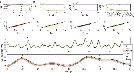
Fig. 9. Identification of the DEA using SVB-NARX, FRO, SEMP and BL. A) The SVB-NARX algorithm selects the optimal model structure at iteration 22 as marked by the dashed line: 15 model terms are selected. B) The ERR for FRO model selection: 12 model terms are selected. C) The MSPE for SEMP model selection: 11 terms are selected. D) The MSPE for the BL algorithm as a function ofλ: 14 model terms are selected (corresponding to the minimum MSPE).
E-H) The system output versus the model predicted output for the models identified by all four algorithms. I) The model predicted output over validation data for the model identified by SVB-NARX (Red) with 95% confidence intervals (Light red shaded area), FRO (Yellow), BL (Purple) and SEMP (Green) with the measured output (Black).
VII. SUMMARY
In this paper a novel approach to nonlinear system identifi-cation of NARX models within a sparse variational Bayesian framework was introduced: The SVB-NARX algorithm. Term selection was driven by the inclusion of a sparsity inducing hyper-prior. We found that the algorithm was relatively fast compared to other nonlinear system identification methods and that it performed successfully even at low SNR levels (down to 2dB). The SVB-NARX algorithm was applied to a real world problem: identification of dielectric elastomer actuators. The algorithm produced an accurate model, and for the first time in nonlinear systems analysis we exploited the Bayesian nature of the SVB-NARX algorithm to numerically propagate the model parameter uncertainty into the nonlinear output frequency response functions.
ACKNOWLEDGMENT
The authors would like to thank the University of Sheffield and the EPRSC for a doctoral training award scholarship to W. Jacobs, which provided funding support for this work. We would like to thank the anonymous reviewers for their helpful comments, which led to a much improved version of this paper.
REFERENCES
[1] I. J. Leontaritis and S. A. Billings, “Input-output parametric models for non-linear systems Part I: deterministic non-linear systems,”International Journal of Control, vol. 41, no. 2, pp. 303–328, Feb. 1985.
[2] S. A. Billings,Nonlinear system identification: NARMAX methods in the time, frequency, and spatio-temporal domains. Wiley, 2013. [3] S. Chen and S. A. Billings, “Representations of non-linear systems: the
NARMAX model,”International Journal of Control, vol. 49, no. 3, pp. 1013–1032, Mar. 1989.
[4] S. Chen, S. A. Billings, and W. Luo, “Orthogonal least squares methods and their application to non-linear system identification,”International Journal of Control, vol. 50, no. 5, pp. 1873–1896, Nov. 1989. [5] S. A. Billings and K. M. Tsang, “Spectral analysis for non-linear systems,
Part I: Parametric non-linear spectral analysis,”Mechanical Systems and Signal Processing, vol. 3, no. 4, pp. 319–339, 1989.
[6] Z. Lang and S. Billings, “Energy transfer properties of non-linear systems in the frequency domain,” International Journal of Control, vol. 78, no. 5, pp. 345–362, 2005.
[7] J. Sj¨oberg, Q. Zhang, L. Ljung, A. Benveniste, B. Delyon, P.-Y. Glorennec, H. Hjalmarsson, and A. Juditsky, “Nonlinear black-box modeling in system identification: a unified overview,” Automatica, vol. 31, no. 12, pp. 1691–1724, 1995.
[8] K. Li, J.-X. Peng, and G. W. Irwin, “A fast nonlinear model identification method,”IEEE Transactions on Automatic Control, vol. 50, no. 8, pp. 1211–1216, Aug 2005.
[9] L. Piroddi and W. Spinelli, “An identification algorithm for polynomial NARX models based on simulation error minimization,”International Journal of Control, vol. 76, no. 17, pp. 1767–1781, Nov. 2003. [10] L. Zhang and K. Li, “Forward and backward least angle regression for
nonlinear system identification,”Automatica, vol. 53, pp. 94–102, 2015. [11] T. Baldacchino, S. R. Anderson, and V. Kadirkamanathan, “Structure
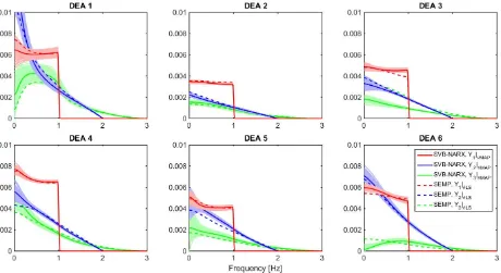
Fig. 10. Analysis of DEA model dynamics in the frequency domain using nonlinear output frequency response functions. The amplitudes of the first three nonlinear output spectra (Y1,Y2andY3) are obtained for each DEA and from each modelling algorithm: SVB-NARX and SEMP.Solid lines: SVB-NARX,
maximum a posteriori(MAP) estimate.Dashed lines: SEMP.Shaded regions: An uncertainty description over each amplitude of the nonlinear output spectra obtained by Monte Carlo sampling from the posterior parameter distribution of the SVB-NARX model and propagated into the frequency domain by evaluating the corresponding nonlinear output spectra (using 100 samples in each case).
and selection operator (lasso) for nonlinear system identification,”IFAC Proceedings Volumes, vol. 39, no. 1, pp. 814–819, 2006.
[13] M. Bonin, V. Seghezza, and L. Piroddi, “NARX model selection based on simulation error minimisation and lasso,”IET Control Theory & Applications, vol. 4, no. 7, pp. 1157–1168, 2010.
[14] V. Peterka, “Bayesian system identification,”Automatica, vol. 17, no. 1, pp. 41–53, 1981.
[15] D. Mackay, “Probable networks and plausible predictions — a review of practical Bayesian methods for supervised neural networks,”Network: Computation in Neural Systems, vol. 6, no. 3, pp. 469–505, Aug. 1995. [16] B. Ninness and S. Henriksen, “Bayesian system identification via Markov chain Monte Carlo techniques,”Automatica, vol. 46, no. 1, pp. 40–51, Jan. 2010.
[17] A. Gelman, Bayesian Data Analysis. Boca Raton, Fl: Chapman & Hall/CRC, 2004.
[18] W. Pan, Y. Yuan, J. Gonalves, and G. B. Stan, “A sparse Bayesian approach to the identification of nonlinear state-space systems,”IEEE Transactions on Automatic Control, vol. 61, no. 1, pp. 182–187, Jan 2016.
[19] P. L. Green and K. Worden, “Bayesian and Markov chain Monte Carlo methods for identifying nonlinear systems in the presence of uncertainty,” Phil. Trans. R. Soc. A, vol. 373, p. 20140405, 2015.
[20] J. L. Beck, “Bayesian system identification based on probability logic,”Journal of International Association for Structural Control and Monitoring, vol. 17, no. 7, pp. 825–847, 2010.
[21] T. Baldacchino, E. J. Cross, K. Worden, and J. Rowson, “Variational Bayesian mixture of experts models and sensitivity analysis for nonlinear dynamical systems,”Mechanical Systems and Signal Processing, vol. 66-67, pp. 178–200, Jan. 2016.
[22] K. Krishnanathan, S. R. Anderson, S. A. Billings, and V. Kadirka-manathan, “Computational system identification of continuous-time
non-linear systems using approximate Bayesian computation,”International Journal of Systems Science, vol. 47, pp. 3537–3544, 2016.
[23] F. Lindsten, T. B. Sch¨on, and M. I. Jordan, “Bayesian semiparametric Wiener system identification,”Automatica, vol. 49, no. 7, pp. 2053–2063, 2013.
[24] R. Frigola and C. E. Rasmussen, “Integrated pre-processing for Bayesian nonlinear system identification with Gaussian processes,” in52nd IEEE Conference on Decision and Control, 2013, pp. 5371–5376.
[25] J. Kocijan, A. Girard, B. Banko, and R. Murray-Smith, “Dynamic systems identification with Gaussian processes,” Mathematical and Computer Modelling of Dynamical Systems, vol. 11, no. 4, pp. 411–424, 2005.
[26] T. Baldacchino, S. R. Anderson, and V. Kadirkamanathan, “Com-putational system identification for Bayesian NARMAX modelling,” Automatica, vol. 49, no. 9, pp. 2641–2651, Sep. 2013.
[27] W. R. Gilks, S. Richardson, and D. J. Spiegelhalter, Eds.,Markov Chain Monte Carlo in Practice. Boca Raton, Fla: Chapman & Hall, 1998. [28] Z. Ghahramani and M. J. Beal, “Propagation algorithms for variational
Bayesian learning,”Advances in Neural Information Processing Systems, pp. 507–513, 2001.
[29] M. I. Jordan, Z. Ghahramani, T. S. Jaakkola, and L. K. Saul, “An introduction to variational methods for graphical models,” Machine Learning, vol. 37, no. 2, pp. 183–233, 1999.
[30] C. M. Bishop and M. E. Tipping, “Variational relevance vector machines,” inProceedings of the Sixteenth Conference on Uncertainty in Artificial Intelligence, 2000, pp. 46–53.
[31] M. E. Tipping, “Sparse Bayesian learning and the relevance vector machine,”The Journal of Machine Learning Research, vol. 1, pp. 211– 244, Sep. 2001.
in cancer diagnosis,”IEEE Transactions on Information Technology in Biomedicine, vol. 11, no. 3, pp. 338–347, 2007.
[33] G.-M. Zhang, D. M. Harvey, and D. R. Braden, “Signal denoising and ultrasonic flaw detection via overcomplete and sparse representations,” The Journal of the Acoustical Society of America, vol. 124, no. 5, pp. 2963–2972, 2008.
[34] H.-Q. Mu and K.-V. Yuen, “Novel sparse Bayesian learning and its application to ground motion pattern recognition,”Journal of Computing in Civil Engineering, vol. 31, no. 5, 2017.
[35] W. R. Jacobs, T. Baldacchino, and S. R. Anderson, “Sparse Bayesian Identification of Polynomial NARX Models,” IFAC-PapersOnLine, vol. 48, no. 28, pp. 172–177, 2015.
[36] A. O’Halloran, F. O’Malley, and P. McHugh, “A review on dielectric elastomer actuators, technology, applications, and challenges,”Journal of Applied Physics, vol. 104, no. 7, p. 071101, 2008.
[37] W. R. Jacobs, E. D. Wilson, T. Assaf, J. Rossiter, T. J. Dodd, J. Porrill, and S. R. Anderson, “Control-focused, nonlinear and time-varying modelling of dielectric elastomer actuators with frequency response analysis,”Smart Materials and Structures, vol. 24, no. 5, p. 055002, May 2015.
[38] E. D. Wilson, T. Assaf, M. J. Pearson, J. M. Rossiter, P. Dean, S. R. Anderson, and J. Porrill, “Biohybrid control of general linear systems using the adaptive filter model of cerebellum,”Frontiers in Neurorobotics, vol. 9, no. 5, 2015.
[39] C. M. Bishop,Pattern Recognition and Machine Learning. New York: Springer, 2006.
[40] J. E. Griffin and P. J. Brown, “Inference with Normal-Gamma prior distributions in regression problems,”Bayesian Analysis, vol. 5, no. 1, pp. 171–188, Mar. 2010.
[41] R. M. Neal, Bayesian Learning for Neural Networks. New York: Springer, 1996.
[42] D. P. Wipf and S. S. Nagarajan, “A new view of automatic relevance determination,” inAdvances in neural information processing systems, 2008, pp. 1625–1632.
[43] S. Sun, “A review of deterministic approximate inference techniques for Bayesian machine learning,”Neural Computing and Applications, vol. 23, no. 7, pp. 2039–2050, 2013.
[44] M. J. Beal, “Variational algorithms for approximate Bayesian inference,” Ph.D. dissertation, University of London, 2003.
[45] J. Drugowitsch, “Variational Bayesian inference for linear and logistic regression,”arXiv preprint, vol. arXiv:1310.5438, 2013.
[46] D. M. Blei and M. I. Jordan, “Variational inference for Dirichlet process mixtures,”Bayesian Analysis, vol. 1, no. 1, pp. 121–144, 2006. [47] J. Friedman, T. Hastie, and R. Tibshirani, “Regularization paths for
generalized linear models via coordinate descent,”Journal of Statistical Software, vol. 33, no. 1, p. 1, 2010.
[48] Y. Bar-Cohen, Ed.,Electroactive polymer (EAP) actuators as artificial muscles: reality, potential, and challenges, 2nd ed. Bellingham, Wash: SPIE Press, 2004.
[49] P. Brochu and Q. Pei, “Advances in Dielectric Elastomers for Actuators and Artificial Muscles,”Macromolecular Rapid Communications, vol. 31, no. 1, pp. 10–36, Jan. 2010.
[50] K. Z. Mao and S. A. Billings, “Algorithms for minimal model structure detection in nonlinear dynamic system identification,” International Journal of Control, vol. 68, no. 2, pp. 311–330, Jan. 1997.
[51] A. Sherstinsky and R. W. Picard, “On the efficiency of the orthogonal least squares training method for radial basis function networks,”IEEE Transactions on Neural Networks, vol. 7, no. 1, pp. 195–200, 1996. [52] G. Rizzello, D. Naso, A. York, and S. Seelecke, “Modeling, identification,
and control of a dielectric electro-active polymer positioning system,” IEEE Transactions on Control Systems Technology, vol. 23, no. 2, pp. 632–643, 2015.
[53] Z.-Q. Lang and S. A. Billings, “Output frequency characteristics of
nonlinear systems,”International Journal of Control, vol. 64, no. 6, pp. 1049–1067, Aug. 1996.
[54] L. O. Chua and C.-Y. Ng, “Frequency domain analysis of nonlinear systems: general theory,”IEE Journal on Electronic Circuits and Systems, vol. 3, no. 4, pp. 165–185, 1979.
William R. Jacobsreceived the M.Phys. degree in physics with mathematics from the University of Sheffield, Sheffield, UK, in 2010 and the Ph.D. degree in nonlinear system identification from the University of Sheffield in 2016.
He is currently working as a Research Associate in the Rolls Royce University Technology Centre, Department of Automatic Control and Systems En-gineering at the University of Sheffield.
Tara Baldacchinoreceived the B.Eng. degree in elec-trical engineering from the Faculty of Engineering, University of Malta, Malta, in 2006 and the M.Sc. degree in control systems and the Ph.D. degree from the Department of Automatic Control and Systems Engineering, University of Sheffield, Sheffield, U.K., in 2008 and 2011, respectively.
From 2011 to 2015 she was a Research Associate in the Dynamics Research Group, Department of Mechanical Engineering, University of Sheffield. She is currently a University Teacher in the Department of Automatic Control and Systems Engineering, University of Sheffield.
Tony Doddreceived the B.Eng. degree in aerospace systems engineering from the University of Southamp-ton, SouthampSouthamp-ton, UK, in 1994 and the Ph.D. degree in machine learning from the Department of Electron-ics and Computer Science, University of Southampton in 2000.
From 2002 to 2010, he was a Lecturer in the Depart-ment of Automatic Control and Systems Engineering at the University of Sheffield, Sheffield, UK, and from 2010 to 2015 was a Senior Lecturer at the University of Sheffield. He is currently a Professor of Autonomous Systems Engineering and Director of the MEng Engineering degree programme at the University of Sheffield.
Sean R. Andersonreceived the M.Eng. degree in control systems engineering from the Department of Automatic Control and Systems Engineering, University of Sheffield, Sheffield, UK, in 2001 and the Ph.D. degree in nonlinear system identification and predictive control from the University of Sheffield in 2005.