https://doi.org/10.5194/acp-18-7393-2018 © Author(s) 2018. This work is distributed under the Creative Commons Attribution 4.0 License.
The impact of biogenic, anthropogenic, and biomass burning volatile
organic compound emissions on regional and seasonal variations in
secondary organic aerosol
Jamie M. Kelly1, Ruth M. Doherty1, Fiona M. O’Connor2, and Graham W. Mann3 1School of GeoSciences, The University of Edinburgh, Edinburgh, UK
2Met Office Hadley Centre, Exeter, UK
3National Centre for Atmospheric Science, School of Earth and Environment, University of Leeds, Leeds, UK Correspondence:Jamie M. Kelly (j.kelly-16@sms.ed.ac.uk)
Received: 16 October 2017 – Discussion started: 7 November 2017
Revised: 24 April 2018 – Accepted: 25 April 2018 – Published: 28 May 2018
Abstract.The global secondary organic aerosol (SOA) bud-get is highly uncertain, with global annual SOA produc-tion rates, estimated from global models, ranging over an order of magnitude and simulated SOA concentrations un-derestimated compared to observations. In this study, we use a global composition-climate model (UKCA) with interac-tive chemistry and aerosol microphysics to provide an in-depth analysis of the impact of each VOC source on the global SOA budget and its seasonality. We further quan-tify the role of each source on SOA spatial distributions, and evaluate simulated seasonal SOA concentrations against a comprehensive set of observations. The annual global SOA production rates from monoterpene, isoprene, biomass burning, and anthropogenic precursor sources is 19.9, 19.6, 9.5, and 24.6 Tg(SOA)a−1, respectively. When all sources are included, the SOA production rate from all sources is 73.6 Tg(SOA)a−1, which lies within the range of estimates from previous modelling studies. SOA production rates and SOA burdens from biogenic and biomass burning SOA sources peak during Northern Hemisphere (NH) summer. In contrast, the anthropogenic SOA production rate is fairly constant all year round. However, the global anthropogenic SOA burden does have a seasonal cycle which is lowest dur-ing NH summer, which is probably due to enhanced wet re-moval. Inclusion of the new SOA sources also accelerates the ageing by condensation of primary organic aerosol (POA), making it more hydrophilic, leading to a reduction in the POA lifetime. With monoterpene as the only source of SOA, simulated SOA and total organic aerosol (OA) concentrations are underestimated by the model when compared to surface
1 Introduction
Organic Aerosol (OA) is important from both air quality and climate perspectives. Measurements across the North-ern Hemisphere (NH) mid-latitudes suggest OA represents between 18 and 70 % of fine aerosol mass depending on location and atmospheric conditions (Zhang et al., 2007). However, due to coarse grid resolutions and uncertainties in the SOA life cycle, global chemistry transport models and general circulation model systematically underpredict ob-served OA concentrations in both urban (mean normalized bias= −62 %) and remote (mean normalized bias= −15 %) environments (Tsigaridis et al., 2014). Therefore, assessment of subsequent OA impacts on air quality (Hodzic et al., 2016) and climate (Scott et al., 2015) suffer from a lack of confi-dence.
OA can be emitted as primary organic aerosol (POA) or formed as secondary organic aerosol (SOA). SOA is formed from the oxidation products of volatile organic compounds (VOCs) and semi volatile and intermediate volatility organic compounds (S/IVOCs). Across the NH mid-latitudes, SOA accounts for 64, 83, and 95 % of observed surface OA sub-micron mass in urban, urban downwind and remote envi-ronments, respectively (Zhang et al., 2007). Despite the ob-served ubiquity of SOA in the atmosphere, models generally perform poorly at reproducing observed SOA concentrations (Tsigaridis et al., 2014). Using either global (Hodzic et al., 2016) or regional (Chen et al., 2009) scale models, relatively good agreement between simulated and observed SOA centrations in remote environments has been found. In con-trast, in urban environments, simulated SOA concentrations are substantially lower than observed (Hodzic et al., 2009; Heald et al., 2011; Khan et al., 2017).
Estimated annual global SOA production rates, based on bottom-up approaches using global models, range from 12 to 480 Tg(SOA)a−1 (Kanakidou et al., 2005; Heald et al., 2011; Tsigaridis et al., 2014; Hodzic et al., 2016; Shrivastava et al., 2015). This large inter-model spread in simulated SOA production rates is likely due to an incomplete understanding of the different sources of SOA and a lack of observations available to constrain models. Global annual SOA produc-tion rates, estimated from top-down methods, such as scal-ing of the sulphate budget (Goldstein and Galbally, 2007), or constraining the SOA budget using satellite data (Heald et al., 2010) or in situ observations (Spracklen et al., 2011), are substantially greater and even more uncertain (range 50– 1820 Tg(SOA)a−1). Uncertainty ranges for the global POA budget are narrower, with estimates of global POA produc-tion ranging from 34 to 144 Tg(POA)a−1(Tsigaridis et al., 2014).
Emitted from both natural and anthropogenic sources, SOA has important climatic impacts. SOA can perturb the energy balance of the Earth by absorption and scattering (aerosol–radiation interactions) and by altering cloud prop-erties (aerosol–cloud interactions) (Forster and Ramaswamy,
2007). However, climatic impacts of SOA are very sensitive to the SOA budget. For example, in a multi-model study, es-timates of the increase in the global SOA burden since prein-dustrial times ranged from 0.09 to 0.97 Tg (SOA), which resulted in a direct radiative effect ranging from −0.21 to
−0.01 W m−2(Myhre et al., 2013). As an aerosol with a large natural source, SOA also contributes to the uncertainty in preindustrial aerosol concentrations, which is the dominant contribution to the uncertainty in the aerosol cloud albedo effect forcing (Carslaw et al., 2013). Hence, reducing uncer-tainty in the SOA budget is crucial for constraining radiative forcing estimates.
The identity of SOA precursors is critical to our under-standing of the SOA budget and its life cycle; however, the dominant precursors of SOA remain highly uncertain in their magnitudes and spatial distributions. Biogenic volatile or-ganic compounds (bVOCs) are considered important sources of SOA due to high emissions (Guenther et al., 2012) and fast reactivity. Laboratory and field studies suggest that monoter-pene (C10H16) (Yu et al., 1999), isoprene (C5H8) (Ng et al., 2008), sesquiterpenes (C15H24) (Tasoglou and Pandis, 2015) and the heterogeneous uptake of glyoxal (Volkamer et al., 2007) are all important biogenic sources of SOA. Global biogenic SOA production rates, estimated using global mod-els, range between 2.86 and 97.5 Tg(SOA)a−1(Henze et al., 2008; Heald et al., 2008; Farina et al., 2010; Hodzic et al., 2016). Isoprene (Bonsang et al., 1992) and monoterpene (Yassaa et al., 2008) are also emitted from phytoplankton. Al-though the SOA production rates from marine VOCs is small, estimated at 5 Tg(SOA)a−1(Myriokefalitakis et al., 2010), marine SOA may be important from a climate perspective due to changes to cloud-condensation nuclei (Meskhidze et al., 2011). Many global models only consider biogenic sources in their formation of SOA (Tsigaridis et al., 2014); other studies that include a number of different precursor types suggest that biogenic sources contribute 74 % (Hodzic et al., 2016) to 95 % (Farina et al., 2010) to the annual global total SOA production rate.
top-down study is in stark contrast to bottom up estimates from global modelling studies. However, it remains unclear whether the anthropogenic dominance of global SOA pro-duction found in Spracklen et al. (2011) simply reflects the location of observations used to constrain this estimate; ob-servations were primarily located in the NH mid-latitudes where anthropogenic emissions are highest. Additionally, the reaction yield required to reach a production rate of 100 Tg(SOA)a−1 of anthropogenic SOA exceeds the re-action yield derived from laboratory studies (Odum et al., 1997). Furthermore, a high SOA production rate from an-thropogenic sources produced positive models biases com-pared to observed SOA concentrations in remote environ-ments (Spracklen et al., 2011) and at higher altitudes (Heald et al., 2011).
Laboratory (Grieshop et al., 2009) and field campaigns (Cubison et al., 2011) suggest biomass burning VOCs and S/IVOCs can form SOA. Using observations, Cubi-son et al. (2011) estimated the global SOA production rate from biomass burning at 1–15 Tg(SOA)a−1. This is consistent with Spracklen et al. (2011), who estimated a global SOA production rate from biomass burning of 3–26 Tg(SOA)a−1 using a top-down approach. S/IVOCs are estimated to account for between 15 and 37 % of biomass burning carbonaceous emissions (Stockwell et al., 2015; Yokelson et al., 2013). Due to the limited knowledge of S/IVOCs emissions and chemistry, assumptions are re-quired when implementing biomass burning S/IVOCs into global models. As a consequence biomass burning SOA pro-duction rates, estimated using global models, range sub-stantially from 15.5 Tg(SOA)a−1 (Hodzic et al., 2016) to 44–95 Tg(SOA)a−1 (Shrivastava et al., 2015). Therefore, biomass burning remains an additional highly uncertain and potentially important source of SOA. Therefore, biomass burning remains an additional highly uncertain and poten-tially important source of SOA.
Anthropogenic and biomass burning emissions include S/IVOCs, which in addition to VOCs, can also contribute to SOA formation (Robinson et al., 2007). As traditional emis-sions inventories, such as van der Werf et al. (2010), account for only a fraction of the emitted S/IVOCs, most modelling studies completely neglect the role of S/IVOCs as sources of SOA. Alternatively, SOA formation from S/IVOCs can be artificially accounted for by scaling up reaction yields of VOCs. Assumptions in the amount of S/IVOCs miss-ing from traditional emissions inventories introduces un-certainty, with estimates ranging from 0.25–2.8 times POA emissions (Robinson et al., 2010; Shrivastava et al., 2008). Estimates of global annual-total S/IVOC emissions range from 54 (Hodzic et al., 2016) to 450 Tg a−1 (Shrivastava et al., 2015). Despite these uncertainties, S/IVOCs have been included in a number of models. Both Hodzic et al. (2016) and Tsimpidi et al. (2016) agree that the sum of the global SOA burden from anthropogenic and biomass burning
pre-cursors is dominated by S/IVOCs (72 and 69 %, respec-tively).
The heterogeneous production of SOA may be an addi-tionally important source of SOA, which is often not in-cluded in models (e.g. see Tsigaridis et al., 2014). Soluble and polar organic vapours, which are too volatile to con-dense, may be taken up by the aqueous phase, either in aerosol liquid water or cloud liquid water. Within the aqueous phase, oxidation may lead to less volatile products which, af-ter liquid evaporation, remain in the aerosol phase (Ervens, 2015). One example of a polar water soluble compound, which is too volatile to directly condense, but may form SOA within the aqueous phase, is glyoxal (Volkamer et al., 2007). Recent estimates of the global annual-total SOA production rate within the cloud and aerosol phases are 13–47 and 0– 13 Tg(SOA)a−1, respectively (Lin et al., 2014, 2012). Aque-ous production may be an important source of SOA, but sev-eral uncertainties remain, including the amount of cloud and liquid water in the atmosphere, and how to simulate the up-take of organic gases onto aqueous surfaces.
The diversity in treatment of SOA formation within global models was highlighted in a recent multi-model study (Tsi-garidis et al., 2014). Of the 31 models included in this study, 11 models treat SOA formation by directly “emitting” SOA from vegetation. In doing so, these schemes neglect the role of many important atmospheric conditions on SOA forma-tion rates. For example, the effect of oxidant levels on both reaction rates and yields of SOA precursors are neglected. Some models simulate SOA precursor emissions and subse-quent oxidation to lower volatility compounds, which then condense to form SOA. In such SOA schemes, the effect of oxidant levels on SOA precursor reaction kinetics are ac-counted for. However, in studies where a single reaction yield is assumed throughout the atmosphere (Chung and Sein-feld, 2002; Tsigaridis and Kanakidou, 2003; Spracklen et al., 2011), the effects of atmospheric conditions on reaction yields are neglected. However, chamber experiments show that SOA yields vary substantially with different atmospheric environmental conditions for each of the main SOA precur-sor species: reaction yields of monoterpenes (Sarrafzadeh et al., 2016), isoprene (Rattanavaraha et al., 2016) and aro-matics (Ng et al., 2007b) are all affected by oxidant levels.
Environmental chambers are typically used to elucidate hydrocarbon oxidation mechanisms and SOA yields. Sev-eral recent advances in SOA environmental chamber studies have been made, including the influence of NOxand
humid-ity on SOA yields. Early estimates of SOA yields from aro-matic compounds, which were conducted in relatively high nitrogen oxide (NOx=NO and NO2) concentrations, range between 5 and 10 % (Odum et al., 1997, 1996). However, more recent studies have shown that SOA yields from aro-matic compounds are strongly influenced by NOx, which has
How-ever, under low-NOxconditions, Ng et al. (2007b) measured
substantially higher SOA yields of 37, 30, and 36 % for ben-zene (C6H6), toluene (C7H8), and xylene (C8H10), respec-tively. Also under low-NOx conditions, Chan et al. (2009)
observed an SOA yield of 73 % from naphthalene (C10H8). Environmental chamber studies have also found similar re-lationships between NOx and SOA yields for several other
important species, including monoterpene (Ng et al., 2007a) and isoprene. In addition, water vapour may also affect SOA yields. For aromatic compounds, both positive (White et al., 2014) and negative (Cocker et al., 2001) correlations between aromatic SOA yields and relative humidity have been ob-served in chamber studies, hence, the role of water vapour in aromatic oxidation is not yet clear. These environmen-tal chamber studies have helped elucidate oxidation mech-anisms, and linked them to the strength of SOA production (i.e. yields). However, global models commonly use a sin-gle SOA yield throughout the atmosphere. Therefore, the demonstration of variable SOA yields in laboratory studies results in greater difficulty in selecting an SOA yield for a global model. Also, within an environmental chamber, up-take of organic compounds by the surface walls (known as “wall losses”) can occur. Traditionally, this process was as-sumed to be non-negligible, resulting in the potential for environmental chamber studies to underestimate the reac-tion yield. Zhang et al. (2014) found that reacreac-tion yields of toluene, an anthropogenic source of SOA, were under estimated by a factor of four due to wall losses during chamber studies. This has a significant effect on simulated SOA production. Updating reaction yields to account for wall losses in global models resulted in an increase in the global annual biogenic SOA production rate from 21.5 to 97.5 Tg(SOA)a−1(Hodzic et al., 2016).
Volatility is another important aspect of OA. Whereas oxidation products from biogenic VOCs are predomi-nantly compounds with extremely low volatility, so-called ELVOCs, (e.g. Ehn et al., 2014), there is considerable ev-idence that anthropogenic SOA is primarily composed of semi-volatile material. A large component of POA is also semi-volatile. For example, combustion POA, either gener-ated from gasoline (May et al., 2013b) or diesel (May et al., 2013c) within laboratory studies suggests POA is primar-ily semi-volatile (i.e. only a small proportion consists of ELVOCs). Also, analysis of POA emitted from the burn-ing of vegetation within laboratory studies suggests POA is semi-volatile (May et al., 2013a). Furthermore, analysis of OA, generated in both laboratories (Huffman et al., 2009b) and field campaigns (Huffman et al., 2009a) suggests OA is semi-volatile. However, some specific cases suggest a pro-portion of OA is non-volatile (Cappa and Jimenez, 2010; Jimenez et al., 2009; Vaden et al., 2011). Considering labora-tory and field studies suggest OA is dominated by the semi-volatile fraction, the treatment of volatility of OA within global models ranges substantially. Of the 31 state-of-the-art global models included in AeroCom, only 12 treat OA as
semi-volatile (Tsigaridis et al., 2014). Recently, the effects of volatility on SOA were quantified in a global modelling study by Shrivastava et al. (2015). These authors estimate that the global annual-total SOA production rate varies by almost a factor of 2 depending on whether OA is treated as semi-volatile or non-volatile. The particle-phase state may be another important factor but is poorly characterized (Shi-raiwa et al., 2017), and is dependent on relative humidity and SOA precursor (Hinks et al., 2016; Bateman et al., 2016). Overall, global models show a clear systematic low bias in simulated SOA concentrations in comparison to observations (Tsigaridis et al., 2014). Current global models represent a broad spectrum in chemical complexity, ranging from es-sentially no chemical-dependence on SOA production up to moderate-complexity SOA mechanisms with volatility basis set (VBS) (Donahue et al., 2006). Whether this systematic underprediction of SOA is due to incomplete SOA sources in the models or underprediction SOA yields is not yet clear. Al-though numerous studies have investigated SOA production in global models, these have mostly focussed on individual sources, with an aim to reduce model biases. Very few stud-ies include all major sources of SOA. Some studstud-ies suggest that the global SOA budget is dominated by biogenic sources (Hodzic et al., 2016), whereas others suggest it is dominated by biomass burning (Shrivastava et al., 2015). Additionally, Spracklen et al. (2011) indicates that biogenic SOA can be “anthropogenically enhanced” in polluted regions.
In this study, a global chemistry and aerosol model (UKCA) is used to simulate SOA concentrations from all the VOC emission source types described above: monoter-pene, isoprene, anthropogenic, and biomass burning. Other mechanisms of SOA production, such as S/IVOCs and het-erogeneous production, may also be important, but in this study, the focus is on VOCs. The novelty of this study is that a global model is used to simulate SOA and POA from a number of different sources, evaluating simulated concen-trations against a consistent set of observations to provide new insights into the seasonal influence of these different SOA precursor sources. The paper is organized as follows: Sect. 2 describes the modelling approach and the measure-ments used to evaluate the model are described in Sect. 3. Results on the global SOA production rates, spatial POA and SOA distributions, and comparisons with surface and aircraft observations are explored in Sect. 4, with discussion and con-cluding remarks in Sect. 5.
2 Chemistry–climate model description
config-uration with prescribed sea surface temperature and sea ice fields based on 1995–2004 reanalysis data (Reynolds et al., 2007). The model is run at a horizontal resolution of N96 (1.875◦ longitude by 1.25◦ latitude). The vertical dimen-sion has 85 terrain-following hybrid-height levels distributed from the surface to 85 km. Horizontal winds and tempera-ture in the model are nudged towards ERA-Interim reanaly-ses (Dee et al., 2011) using a Newtonian relaxation technique with a relaxation time constant of 6 h (Telford et al., 2008). There is no feedback from the chemistry or aerosols onto the dynamics of the model; this ensures identical meteorology across all simulations, so that differences in modelled SOA concentration are solely due to differences in SOA sources.
The UK Chemistry and Aerosol (UKCA) model used in this study combines the “TropIsop” tropospheric chemistry scheme from O’Connor et al. (2014) with the stratospheric chemistry scheme from Morgenstern et al. (2009). There are 75 species with 285 reactions. This includes odd oxygen (Ox), nitrogen (NOy), hydrogen (HOx=OH+HO2), and carbon monoxide (CO). Hydrocarbons included are methane, ethane, propane, isoprene and monoterpene. Isoprene oxida-tion follows the Mainz Isoprene Mechanism (Poschl et al., 2000) which is described in detail in O’Connor et al. (2014). The aerosol component of UKCA is the 2-moment modal version of the Global Model of Aerosol Processes (GLOMAP-mode) (Mann et al., 2010). Aerosol components considered are sulphate (SO4), sea salt (SS), black carbon (BC), primary organic aerosol (POA) and secondary organic aerosol (SOA). Both aerosol mass and number are trans-ported in seven internally mixed log-normal modes (four soluble and three insoluble). Aerosol growth occurs via nucleation, coagulation, condensation, ageing, hygroscopic growth and cloud processing. Condensation ageing trans-fers hydrophobic particles into the hydrophilic mode when a 10-monolayer is formed on the surface a hydrophobic par-ticle. Dry deposition and gravitational settling of aerosol follows Slinn (1982) and Zhang et al. (2012), respectively. Grid-scale wet deposition of aerosol occurs via nucleation scavenging and impact scavenging. Subgrid-scale wet depo-sition occurs via plume scavenging (Kipling et al., 2013). New particle formation by binary homogenous nucleation of sulphuric acid (H2SO4) follows that described by Kul-mala et al. (2006). Gaseous sulphur compounds (sulphur dioxide, SO2 and dimethyl sulphide, DMS) and VOCs are oxidized, forming low volatility gases which condense ir-reversibly onto pre-existing aerosol. Condensation is calcu-lated following Fuchs (1971) which is described in Mann et al. (2010). Mineral dust is treated by the model in a sepa-rate aerosol module (Woodward, 2001).
The emissions used are all decadal-average emissions, centred on the year 2000, and monthly varying. Anthro-pogenic and biomass burning gas-phase emissions are pre-scribed following Lamarque et al. (2010). Biogenic emis-sions of isoprene, monoterpene and methanol (CH3OH) are also prescribed, taken from the Global Emissions Inventory
Activity (GEIA), based on Guenther et al. (1995). A diurnal cycle in isoprene emissions is imposed. POA and BC emis-sions from fossil fuel combustion are prescribed following Lamarque et al. (2010). POA and BC emissions from sa-vannah burning and forest fires are prescribed, taken from the Global Fire Emissions Database (GFEDv2; van der Werf et al., 2010). All carbonaceous emissions are emitted into the insoluble mode and are transferred to the soluble mode by condensation ageing. Ageing proceeds at a rate consistent with a 10-monolayer coating being required to make a parti-cle soluble.
2.1 Formation of SOA in the standard version of the model
In UKCA, VOCs undergo oxidation ([o]=OH, O3 and NO3). VOC oxidation products considered with a low enough volatility to condense are represented by a single sur-rogate compound, SOG. The reaction yield (α) describes the molar quantity (stoichiometric coefficient) of low volatility vapours formed. SOG condenses irreversibly onto the surface of pre-existing aerosol, calculated following Fuchs (1971).
VOC+ [o] →αSOG→SOA (1)
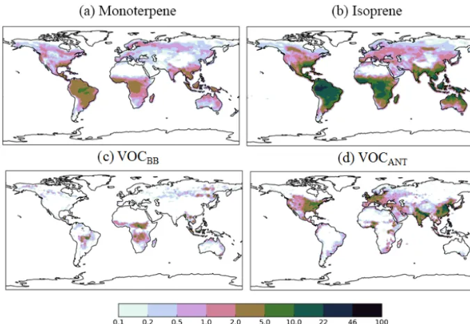
In this study, as with the majority of global aerosol models (e.g. Tsigaridis et al., 2014), OA is treated as a non-volatile species, the emission or chemical yield implicitly reflecting only the particle phase component of OA. As we discuss in Sect. 1, anthropogenic OA in particular has a substantial semi-volatile component, which will introduce an important mode of variability to aerosol properties in industrial regions. In UKCA, monoterpenes (C10H16), are the only VOC con-sidered in SOA formation. Monoterpene is oxidized, follow-ing reaction kinetics taken from Atkinson et al. (1989). The reaction yield applied to monoterpenes was assumed to be 13 %, which is identical to other global modelling studies (Mann et al., 2010; Scott et al., 2014, 2015), which was taken from Tunved et al. (2006), who estimate the yield at 10–13 %. Global annual monoterpene emissions are 142 Tg (monoter-pene) a−1and their spatial distribution is shown in Fig. 1. 2.2 New SOA sources
Figure 1.Annual-total SOA precursor emissions from the different global VOC sources; monoterpene and isoprene taken from Guenther et al. (1995), VOCBBtaken from EDGAR, and VOCANTtaken from Lamarque et al. (2010). Units are g (VOC) m−2a−1.
biomass burning source of SOA is hereafter referred to as VOCBB. Anthropogenic emissions of aromatic com-pounds, benzene, dimethylbenzene, and trimethylbenzene, were taken from Lamarque et al. (2010) and used to-gether to define the spatial distribution for the anthropogenic source of SOA. These were scaled to reproduce the global annual anthropogenic VOC total emissions estimated by EDGAR (127 Tg(VOC)a−1). This represents the anthro-pogenic source of SOA and will be referred to as VOCANT.
The anthropogenic and biomass burning VOCs are lumped species, which results in difficulty in selecting reaction ki-netics for these species. The VOCs released from anthro-pogenic and biomass burning have a range of carbon-carbon bonding types, with a range of carbon chain length, and a range of functional groups. The exact speciation of these mixtures has not been resolved, especially for higher molec-ular weight species (Yokelson et al., 2013). However, more recent measurements of biomass burning (Stockwell et al., 2015; Hatch et al., 2017) and vehicle fuel emissions (May et al., 2014; Y. L. Zhao et al., 2015) in laboratory condi-tions reveal substantial quantities of oxygenated aliphatic, aromatic (e.g. benzene, toluene), polycyclic aromatic (e.g. naphthalene), furans, as well as large fractions of unknown species. Considering this range in chemical speciation, two compounds were used to represent the reactivity of the an-thropogenic and biomass burning precursors in this study – naphthalene and monoterpene. For all simulations, VOCANT and VOCBB are assumed to react solely with OH. Initially, VOCANT and VOCBBare assumed to have identical reactiv-ity to monoterpene. As monoterpene is a relatively reactive
Figure 2. Seasonality of global SOA precursor emissions from the different VOC sources: monoterpene (red), isoprene (black), VOCANT(blue), and VOCBB(green) (Tg (VOC) month−1).
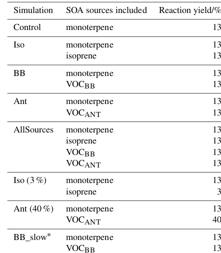
Table 1.Reaction kinetics for SOA precursors in UKCA.
Reaction Rate coefficient (cm3s−1) monoterpene+OH 1.2×10⁻¹¹exp
444
T
monoterpene+O3 1.01×10⁻¹⁵exp
−732
T
monoterpene+NO3 1.19×10⁻¹²exp
490
T
isoprene+OH 2.7×10⁻¹¹exp390T isoprene+O3 1×10⁻¹⁴exp−1995T isoprene+NO3 3.15×10⁻¹²exp
−450
T
VOCANT+OH 1.2×10⁻¹¹exp
444
T
VOCBB+OH 1.2×10⁻¹¹exp
444
T
40 %, which is motivated by the widespread model negative bias in urban environments among global modelling studies. The spatial pattern of precursor emissions from these ad-ditional SOA sources is also shown in Fig. 1. The seasonal cycle of the global precursor emissions from all of the VOC sources is shown in Fig. 2. Biogenic and biomass burning emissions peak during NH summer, whereas anthropogenic emissions are highest during NH spring and winter. Rate co-efficients are taken from Atkinson et al. (1989) and are sum-marized in Table 1.
2.3 Model simulations
Eight model simulations were performed using the differ-ent VOC sources of SOA for two years (1999–2000). The first year was discarded as spin up and the analysis is based on the year 2000 (Table 2). For all SOA components and across all simulations, SOA is solely removed by wet and dry deposition. The control simulation (Control) uses
monoter-Table 2.Summary of simulations carried out in study. Reaction
ki-netics for each source are shown in Table 1. For the BB_Slow simu-lation, VOCBBassumes the reactivity of naphthalene (Atkinson and Arey, 2003).
Simulation SOA sources included Reaction yield/%
Control monoterpene 13
Iso monoterpene 13
isoprene 13
BB monoterpene 13
VOCBB 13
Ant monoterpene 13
VOCANT 13
AllSources monoterpene 13
isoprene 13
VOCBB 13
VOCANT 13
Iso (3 %) monoterpene 13
isoprene 3
Ant (40 %) monoterpene 13
VOCANT 40
BB_slow∗ monoterpene 13
VOCBB 13
pene as the only SOA precursor. Isoprene (its biogenic ter-restrial source only), VOCBB and VOCANT are introduced in additional simulations: Iso, BB, and Ant, respectively. All sources of SOA are combined in the AllSources simulation. A number of sensitivity simulations were also carried out. The first sensitivity study tests a lower isoprene reaction yield of 3 % (Iso (3 %)), which is suggested by laboratory data (Kroll et al., 2005, 2006). The second sensitivity study tests a higher VOCANTreaction yield of 40 % (Ant (40 %)), which is suggested by Spracklen et al. (2011). Another study has also investigated such a large anthropogenic SOA source; however, this was done by scaling simulated anthropogenic SOA concentrations (Heald et al., 2011). A final sensitivity study tests the influence of the assumed reactivity of VOCBB on SOA. Here, with a reaction yield of 13 %, the reactivity is assumed to be identical to naphthalene. Naphthalene was chosen as it has been used as a surrogate compound to rep-resent IVOCs in a global modelling study (Pye and Seinfeld, 2010) and it is roughly 50 % less reactive than monoterpene (Atkinson and Arey, 2003). Three observations are used to evaluate modelled OA.
3 Observations
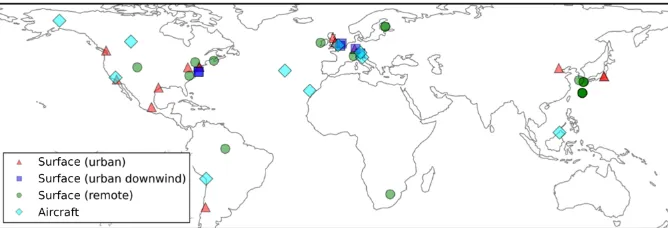
[image:7.612.316.537.118.371.2] [image:7.612.69.262.321.472.2]Figure 3. Global map showing the 40 surface AMS observations, originally compiled by Zhang et al. (2007), classified as urban (red triangles), urban downwind (blue squares), or remote (green circles). Of the surface observations, 37 have been classified as hydrocarbon-like OA and OOA. Observations from 10 aircraft campaigns, originally compiled by Heald et al. (2011), are also shown (light blue diamonds); these remain as total OA.
Spectrometer (AMS) (Canagaratna et al., 2007; Jayne et al., 2000). Uncertainties in the observed OA mass concentration are estimated to be ∼30–35 % (Bahreini et al., 2009). Observations can be accessed on the AMS global network website 2.2 (https://sites.google.com/site/ amsglobaldatabase/, last access: 18 May 2018).
Surface OA observations from the AMS network, origi-nally compiled by Zhang et al. (2007), span the time pe-riod 2000–2010. The 37 observed surface measurement lo-cations are shown in Fig. 3 and coloured according to the en-vironment that they were sampled from: urban, urban down-wind, or remote. Note that, for some sites, multiple measure-ments were made at different time periods. Surface OA mass concentrations were analyzed further using positive matrix factorisation (PMF) to classify OA as either oxygenated OA (OOA) or hydrocarbon-like OA (HOA). We assume observed OOA is comparable to simulated SOA, and observed HOA is comparable to simulated POA. This assumption is made in several other studies (Hodzic et al., 2016; Tsimpidi et al., 2016). The dataset is supplemented with three additional ob-servations of total OA over Santiago (Chile) (Carbone et al., 2013), Manaus (Brazil) (Martin et al., 2010), and Welgegund (South Africa) (Tiitta et al., 2014). These were included as they expand the geographical coverage over which the model can be evaluated. To compare UKCA results to observations spatially, the nearest model grid box (based on its centre co-ordinates) to the measurement site location was selected. The month in which the observations fall is compared to the sim-ulated monthly mean concentration for the year 2000. Note that comparing simulated OA in the year 2000 with mea-sured OA from a different year may introduce discrepancies for model–observation comparison. This is particularly im-portant for regions influenced by biomass burning, as inter-annual variability of biomass burning emissions is extremely high (Tsimpidi et al., 2016). However, simulating the entire measurement period was not possible.
Aircraft OA concentrations from the AMS network, originally compiled by Heald et al. (2011), are also shown in Fig. 3. For details and references of aircraft campaign
(see, https://sites.google.com/site/amsglobaldatabase/). These measurements originate from 10 intensive campaigns worldwide over the period 2000–2010. Four campaigns were carried out in remote regions, located over the northern Atlantic Ocean (TROMPEX and ITOP), Borneo (OP3), and the tropical Pacific Ocean (VOCALS-UK). Three campaigns were carried out in North America and were influenced heavily by biomass burning (ARCTAS-A, ARCTAS-B and ARCTAS-CARB). Three campaigns were also carried out in polluted regions of Europe (EUCAARI, ADIENT and ADRIEX). To compare against UKCA, aircraft observations were binned onto the model’s vertical grid. The nearest model grid box to the average horizontal aircraft measure-ment location was selected for comparison. Again the month of the observations were matched to the monthly mean estimate for 2000 simulated by UKCA. As with the surface evaluation, note the mismatch in measurement and simula-tion years as a potential contributor to model–observasimula-tion discrepancies.
4 Results and discussion 4.1 Global SOA budget
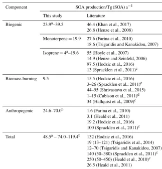
Table 3.Global annual SOA production from this study and the literature (Tg (SOA) a−1). In this study, estimates derived from the isoprene (Iso (3 %)) and anthropogenic (Ant (40 %)) sensitivity simulations in this study are indicated. All remaining estimates from this study are based on simulations using identical reaction yields of 13 %. From the literature, estimates derived from top-down and observation methods are indicated. The remaining estimates form the literature are based on bottom-up approaches.
Component SOA production/Tg(SOA)a−1 This study Literature
Biogenic 23.9a–39.5 46.4 (Khan et al., 2017) 26.8 (Henze et al., 2008)
Monoterpene=19.9 27.6 (Farina et al., 2010)
18.6 (Tsigaridis and Kanakidou, 2007)
Isoprene=4a–19.6 55 (Hoyle et al., 2007)
14.9 (Henze and Seinfeld, 2006) 97.5 (Hodzic et al., 2016) 13 (Spracklen et al., 2011)c Biomass burning 9.5 15.5 (Hodzic et al., 2016)
3–26 (Spracklen et al., 2011)c 44–95 (Shrivastava et al., 2015) 1–15 (Cubison et al., 2011)d 34 (Hallquist et al., 2009)c Anthropogenic 24.6–70.0b 1.6 (Farina et al., 2010)
3.1 (Heald et al., 2011) 19.2 (Hodzic et al., 2016) 100 (Spracklen et al., 2011)c Total 48.5a– 74.0–119.4b 132 (Hodzic et al., 2016)
19 (13–121) (Tsigaridis et al., 2014) 12–70 (Tsigaridis and Kanakidou, 2007) 140 (50–380) (Spracklen et al., 2011)c 250 (50–450) (Heald et al., 2010)c 26.5 (Heald et al., 2011)
280–1820 (Goldstein and Galbally, 2007)c
aEstimated using an isoprene yield of 3 %.bEstimated using an anthropogenic yield of 40 %.cEstimated using
top-down methods.dEstimated using observations.
with relatively lower concentrations over the Amazon and Congo, and higher concentrations over continental regions of the NH. Additionally, the short-lived oxidants, OH and NO3, have strong diurnal profiles. In contrast, O3is more tempo-rally homogeneous. VOC emissions are also spatially vari-able; in tropical forests, emissions of isoprene exceed emis-sions of monoterpene, whereas, in boreal forests, emisemis-sions of monoterpene exceed emissions of isoprene. The response of bVOCs to regional and temporal oxidant concentration variability, together with differences in reaction constants for oxidation (Table 1) explains why SOA production from isoprene, despite its higher emissions compared to monoter-pene, has similar SOA production rates.
With isoprene and monoterpene as sources of SOA, the global annual biogenic SOA production rate is 39.5 Tg(SOA)a−1(Table 3). This is in reasonable agreement with estimates of biogenic SOA production from most other global modelling studies (14.9–55 Tg(SOA)a−1; Table 3),
despite possible differences in which biogenic VOCs are in-cluded in the SOA schemes. One global modelling study suggests an annual global biogenic SOA production rate of 97.5 Tg(SOA)a−1(Hodzic et al., 2016; Table 3), based on reaction yields that account for wall losses during chamber studies. In contrast, an observationally constrained top-down estimate of biogenic SOA production (13 Tg(SOA)a−1; Ta-ble 3) is much lower than our estimate. In our sensitivity simulation, when the reaction yield describing SOA forma-tion from isoprene is reduced to 3 %, the annual global bio-genic SOA production rate decreases to 23.9 Tg(SOA)a−1 (Table 3), which is still consistent with other global mod-elling studies.
top-down estimate (100 Tg(SOA)a−1) from Spracklen et al. (2011). In our sensitivity simulation when SOA for-mation from anthropogenic sources is increased from 13 to 40 %, the annual global SOA production rate increased to 70.0 Tg(SOA)a−1. Compared to other sources, biomass burning is the smallest source of SOA, yet still signifi-cant (9.5 Tg(SOA)a−1; Table 3). The magnitude of SOA production from biomass burning is consistent with obser-vations (1–15 Tg(SOA)a−1; Table 3) and top-down stud-ies (3–34 Tg(SOA)a−1; Table 3). However, biomass burn-ing SOA production rates vary substantially from different modelling studies. The reason for such large differences be-tween Hodzic et al. (2016) and Shrivastava et al. (2105), both of which simulate biomass burning SOA formation from S/IVOCs, could be due to the lack of knowledge of S/IVOCs emissions and chemistry, resulting in the need for assump-tions when including SOA formation from these species in models (Shrivastava et al., 2017). When all sources of SOA are included with identical reaction yields, the an-nual global SOA production rate is 74.0 Tg(SOA)a−1. This lies within the range of other estimates based on bottom-up methods (13–132 Tg(SOA)a−1; Table 3). However, top-down approaches, such as scaling of the sulphate budget (Goldstein and Galbally, 2007), or constraining the SOA budget by satellite (Heald et al., 2010), in situ observa-tions (Spracklen et al., 2011) are substantially greater (50– 1820 Tg(SOA)a−1; Table 3).
With identical reaction yields, the annual-average global SOA burden, from monoterpene, isoprene, biomass burning, and anthropogenic precursors is 0.19, 0.22, 0.13 and 0.38 Tg (SOA), respectively. With monoterpene only, the annual av-erage global lifetime of SOA is 3.5 days. Inclusion of iso-prene and biomass burning as sources of SOA has little effect on the SOA lifetime, with annual-average global lifetime of SOA ranging from 3.7 to 4.0 days in these simulations. How-ever, inclusion of an anthropogenic source of SOA increases the SOA lifetime to 4.7 days, and to 5.1 days with an anthro-pogenic source with a 40 % yield. The effect of new sources of SOA on SOA lifetime suggest that SOA from monoter-pene, isoprene, and biomass burning has a similarly short lifetime, whereas SOA from anthropogenic sources has a rel-atively longer lifetime.
The variation in lifetime for the different SOA compo-nents is likely due to differences in the spatial distributions of SOA precursor emissions, as well as the extent of co-location of emissions and precipitation. Biogenic and biomass burn-ing VOCs, primarily located in tropical forest regions of the Southern Hemisphere, experience different precipitation rates compared to anthropogenic VOCs, which are primar-ily released in urban and industrial regions of the Northern Hemisphere. Vertical gradients in SOA production can also affect the SOA lifetime. However, in this study, all SOA pre-cursors are emitted at the surface, hence the various SOA components in this study likely have very similar vertical gradients. Shrivastava et al. (2105) find that the SOA lifetime
substantially increases when biomass burning precursors are emitted at higher altitudes. The range in SOA lifetimes over the different simulations in this study is in agreement with Tsigaridis et al. (2014), which ranged from 2.4–15 days. These SOA lifetimes are also in good agreement with Hodzic et al. (2016) who estimate the SOA lifetime from biogenic VOCs, anthropogenic and biomass burning VOCs combined, and anthropogenic and biomass burning S/IVOCs to be 2.2, 3.3 and 3.0 days, respectively.
The simulated global annual cycle of SOA production and SOA burden from varying sources of SOA is shown in Fig. 4. Figure 4 shows biogenic and biomass burning SOA pro-duction peaking during NH summer (Fig. 4a). This is due to both high emissions (Fig. 2) and elevated photochem-istry during this season. This results in both biogenic and biomass burning SOA burdens also peaking during this sea-son (Fig. 4b). The seasea-sonal cycle of the biomass burning SOA is consistent with Tsimpidi et al. (2016). The global SOA production rate and the SOA burden were also found to peak during NH summer in the multi-model study by Tsi-garidis et al. (2014); however the seasonal cycle of SOA production and SOA burden for different SOA components could not be determined. The anthropogenic emissions peak during NH spring and winter (Fig. 2), and are offset by the seasonal cycle of photochemistry (that influences oxida-tion), resulting in constant anthropogenic SOA production all year round (Fig. 4a). However, the anthropogenic SOA bur-den shows a pronounced seasonal cycle with a double peak during spring and autumn and a minimum during summer (Fig. 4b). Therefore, the seasonality of the anthropogenic SOA burden must be driven by the seasonality of the anthro-pogenic SOA lifetime, since it differs from the seasonal cy-cle of SOA production. Indeed, anthropogenic SOA precur-sor emissions are highest over China and India (Fig. 1). Over these regions, during summer, rainfall is greatest, which may result in a reduction in SOA lifetime due to greater wet depo-sition and a decrease in SOA burden. The seasonal profile of the global anthropogenic SOA burden is in agreement with that found by Tsimpidi et al. (2016); however, they suggest an alternative cause. In their model, SOA is treated as semi volatile and can partition between the aerosol and gas-phase (as opposed to in this study, where SOA is treated as non-reactive and non-volatile). In their study, partitioning is de-pendent on a number of parameters, including temperature. Tsimpidi et al. (2016) suggest that the summertime peak in photochemistry is compensated for by enhanced SOA evap-oration. Further research is required to quantify the relative importance of each mechanism on the SOA burden.
4.2 Effects of new SOA sources on simulated SOA and POA spatial distributions
sim-Figure 4.Monthly average global SOA(a)production (Tg (SOA) month−1) and(b)burden (Tg (SOA)), simulated by UKCA for the control simulation in black. For the other UKCA simulations described in Table 2, the monthly average global SOA production and burden are shown relative to the control simulation.
Figure 5.Annual-average surface SOA concentrations (µg m−3) for Control (monoterpene) and AllSources (monoterpene, isoprene, VOCBB,
and VOCANT) simulations described in Table 2.
ulated with a monoterpene source of SOA alone (Control) and with all sources of SOA (monoterpene, isoprene, VOCBB and VOCANT) (AllSources) (Table 1). In the monoterpene only simulation, annual-average surface SOA concentrations range between 3 and 6 µg m−3 over tropical forest regions of South America and Africa, as well as lower SOA con-centrations of up to 3 µg m−3 in the southeastern USA, and in parts of northern India, China, and South East Asia (Fig. 5a). These patterns generally reflects the location of peak monoterpene emissions (Fig. 1), which are emitted by vegetation only in the emissions inventory used here. Fast SOA production from monoterpene and a relatively short lifetime of SOA results in SOA concentrations peaking at the emissions source with a sharp decrease downwind. The addi-tion of new SOA sources (isoprene, VOCBB, and VOCANT) together alongside monoterpene roughly doubles annual-average surface SOA concentrations compared to simula-tions with monoterpene only. In particular, over the Ama-zon and Congo regions, annual average surface SOA con-centrations peak between 5 and 10 µg m−3 (Fig. 5b). Over
industrialized and urban regions of India and China, annual-average surface SOA concentrations exceed 10 µg m−3. Over large parts of the USA, Europe, and most of Asia, SOA con-centrations exceed 0.6 µg m−3(Fig. 5b).
[image:11.612.129.468.288.421.2]bio-Figure 6.Differences in annual-average SOA concentrations (µg m−3) relative to the control run for simulations;(a)AllSources,(b)Iso, (c)BB, and(d)Ant Simulations are described in Table 2.
genic sources of SOA (monoterpene and isoprene) produce SOA concentrations that typically range from 3–10 µg m−3 (Figs. 6b and 5a), which is in agreement with other studies (Hodzic et al., 2016; Shrivastava et al., 2015; Farina et al., 2010). However, Spracklen et al. (2011) suggests that bio-genic sources yield only a small amount of SOA (global pro-duction=13 Tg a−1; Table 3) and, therefore, simulated SOA concentrations in this region in their study did not exceed 1 µg m−3(Spracklen et al., 2011).
Biomass burning SOA also peaks in tropical forest re-gions of South America and the Congo region of Africa (Fig. 6c), corresponding to regions of intense forest and sa-vannah fires (Fig. 1). Over this region, annual average surface SOA concentrations from biomass burning typically range from 1–3 µg m−3(Fig. 6c) and have lower values compared to SOA concentrations arising from the two biogenic sources. Biomass burning also contributes 0.2–1 µg m−3 to annual-average surface SOA concentrations over boreal forests of northern China and Eastern Siberia. The location and magni-tude of these peak SOA concentrations is in agreement with other global modelling and observationally constrained stud-ies (Tsimpidi et al., 2016; Spracklen et al., 2011) despite differences in biomass burning production rates (Table 3), highlighting the importance of SOA lifetimes in determining SOA concentrations.
The inclusion of an anthropogenic source of SOA creases SOA concentrations over much of the NH. Over in-dustrialized and urban regions of China and India, annual-average surface anthropogenic SOA concentrations typically
exceed 6 µg m−3 (Fig. 6d). The location of peak annual-average surface anthropogenic SOA concentrations, which is reflected by the location of anthropogenic combustion emis-sions (Fig. 1), is in agreement with other global modelling studies (Spracklen et al., 2011; Tsimpidi et al., 2016; Hodzic et al., 2016). The magnitude of peak SOA concentrations are lower than Tsimpidi et al. (2016) but consistent with that of Spracklen et al. (2011). The inclusion of an anthropogenic source of SOA also results in increases in annual-average sur-face SOA concentrations in remote regions: between 0.1 and 0.6 µg m−3over the North Atlantic and Pacific Oceans with larger values across the Indian Ocean (>1 µg m−3).
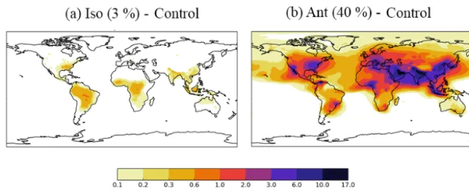
[image:12.612.129.468.60.311.2]concen-Figure 7.Differences in annual-average SOA concentrations (µg m−3) relative to the control run for further sensitivity simulations,(a)Ant (40 %) and(b)Iso (3 %). Simulations are described in Table 2.
Figure 8.Annual-average surface(a)total (hydrophilic and hydrophobic) and(b)hydrophobic only, POA concentrations (µg m−3) for the
Control simulation. Within UKCA, all POA is emitted into the hydrophobic modes and re-distributed into the hydrophilic modes through condensation-ageing.
trations increases by up to 17 µg m−3across most industri-alized regions relative to the monoterpene only simulation (Fig. 7b). The magnitude of these peak SOA concentrations are in broad agreement with Tsimpidi et al. (2016). Con-trastingly, our peak simulated anthropogenic SOA concentra-tions exceed those from the Spracken et al. (2011) study, de-spite our smaller production rate (Table 3), again suggesting the importance of differences in SOA lifetime in determin-ing SOA concentrations. For an increase in reaction yield of a factor of three, surface SOA concentrations increase by the same amount, further corroborating the linear dependence of surface concentrations on reaction yield, as observed in the isoprene sensitivity simulation.
The SOA spatial distributions simulated in this study may be sensitive to the assumption of fast reaction kinetics for an-thropogenic and biomass burning SOA precursors. Here, we have assumed anthropogenic and biomass burning sources of SOA are oxidized on a timescale identical to that of monoter-pene. This is due to limited information on the identity of dominant SOA precursors from these sources. The influence of assumed reactivity on simulated SOA from biomass burn-ing was investigated in an additional sensitivity simulation
where VOCBBadopts the reactivity of naphthalene (Table 2; Sect. 2.3), an aromatic species which has been used as a sur-rogate compound for IVOCs (Pye and Seinfeld, 2010). Com-pared to monoterpene, naphthalene is roughly 50 % less re-active (Atkinson and Arey, 2003). However, despite this sub-stantial reduction in reactivity, the global annual-total SOA production rate from biomass burning VOCs is reduced by less than 1 %. Also, the simulated spatial distributions are almost identical for the two VOCBB species. Like all other SOA precursors in this study, VOCBBdoes not undergo dry or wet deposition. Therefore, a reduction in the reactivity of VOCBBdoes not affect the fate of this compound.
[image:13.612.130.468.251.383.2](con-Figure 9.Differences in annual average surface total POA concentrations (µg m−3) relative to the control run for the following simulations: (a)AllSources,(b)Iso,(c)BB, and(d)Ant, which are described in Table 2. Regions of decreased POA correspond to regions of increased SOA concentrations, availability of hydrophobic POA and efficient wet removal.
densation ageing). UKCA assumes 10 monolayers of solu-ble material are required to redistribute hydrophobic parti-cles into the hydrophilic mode. Over the Amazon, total POA lies in the range of 0.34–2.2 µg m−3 and is almost entirely hydrophilic (Fig. 8a and b). This is due to sufficiently high SOA concentrations in the monoterpene-only source simu-lation, which also peak in this same region (Fig. 5a). Over the Congo region, total POA concentrations lie between 1.2 and 4 µg m−3(Fig. 8a) and hydrophobic POA concentrations range from 0.17 to 1.51 µg m−3 (Fig. 8b). In this region, SOA concentrations are high enough (Fig. 5a) to re-distribute the majority of POA into the hydrophilic mode; however, a small amount remains in the hydrophobic mode. Over northern China and eastern Siberia, total POA concentrations are extremely high, ranging from 4 to 25 µg m−3(Fig. 8a). In this region, SOA concentrations are low (Fig. 5a), there-fore, a substantial fraction of POA remains in the
hydropho-bic mode (range 2.59–13.2 µg m−3(Fig. 8b). Overall, 25 % of the global annual-average POA burden is hydrophobic.
[image:14.612.132.467.61.438.2]Over the Amazon, although inclusion of isoprene and biomass burning results in substantial increases in SOA con-centrations (Fig. 6b and c), there are negligible changes in POA concentrations (Fig. 9). In this region of the world, in the monoterpene only simulation, the majority of POA is hy-drophilic. For this reason, increased SOA concentrations in this region have no effect on the partitioning of POA be-tween the hydrophobic and hydrophilic modes, hence there is little change in POA lifetime. Over urban and industrial-ized regions of India and China, hydrophobic POA concen-trations are much higher (Fig. 8b). In these regions, the inclu-sion of isoprene and anthropogenic sources of SOA results in substantial increases in SOA concentrations (Fig. 6b and d), therefore, hydrophilic POA concentrations in this region are increased. However, there are minimal changes in annual-average surface total POA concentrations (Fig. 9) which is probably due to inefficient wet removal. Across all simula-tions, in various locasimula-tions, inclusion of new sources of SOA reduces POA concentrations. However, the decrease in POA concentrations is always outweighed by the increase in SOA concentrations, thus total OA increases.
To summarize, with monoterpene emissions only, SOA concentrations peak in the SH over tropical forest re-gions of South America and Africa. Including isoprene, biomass burning, and anthropogenic sources of SOA re-sults in substantial increases in SOA concentrations. Iso-prene and biomass burning sources of SOA produce sub-stantial increases in SOA concentrations over the Amazon and Congo compared to the monoterpene only source. The anthropogenic source of SOA increases SOA concentrations over industrialized and urban regions of China, India, USA and Europe. Sensitivity studies show that SOA concentra-tions respond linearly to changes in reaction yields. Upon inclusion of new SOA sources, increased SOA concentra-tions lead to decreased POA concentraconcentra-tions; however, in all regions of the globe, modelled total OA increases.
4.3 Effects of new SOA sources on model agreement with observations
In this section, simulated SOA, POA, and total OA concen-trations (see Sect. 4.2), are evaluated against observations (see Sect. 3). First, simulated SOA and POA concentrations are compared to surface measurements. Next, to expand the spatial coverage of evaluation, simulated total OA concen-trations are compared against surface observations. Finally, vertical profiles of simulated total OA concentration are com-pared against aircraft campaign observations.
4.3.1 Evaluation of surface SOA and POA concentrations
Surface observations used to evaluate the model are shown in Fig. 3. Note that the overall number of sites is small and the measurement locations are primarily in NH mid-latitude
re-gions where anthropogenic emissions are high (Fig. 1). How-ever, these sites sample urban, urban downwind, and remote environments over Europe, North America, and Asia. The mean and normalized mean bias (NMB) are used to evaluate model agreement with observations. A summary of statistics evaluating simulated SOA, POA, and OA are shown in Ta-bles 4, 5 and 6, respectively.
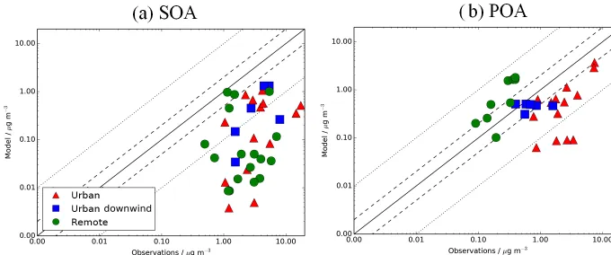
High SOA concentrations observed in urban envi-ronments (mean=4.76 µg m−3) are maintained further downwind (mean=3.93 µg m−3) and in remote envi-ronments (mean=2.70 µg m−3) (Table 4). Contrastingly, observed POA concentrations peak in urban environ-ments (mean=2.79 µg m−3) but decrease rapidly further downwind (mean=0.78 µg m−3) to almost negligible val-ues in remote environments (mean=0.14 µg m−3). Zhang et al. (2007) suggest that cities act as sources of POA, whereas both cities and remote environments are sources of SOA. Compared to other cities, observed SOA and POA are extremely high in densely populated cities. For example, ob-served SOA concentrations in Beijing and Mexico City are 17.3 and 14.55 µg m−3, respectively, roughly 3 times greater than the mean observed SOA in urban environments. Ob-served POA concentrations in Beijing and Mexico City are 7.4 and 7.23 µg m−3, respectively, roughly 2.5 times greater than the mean observed POA in urban environments.
Figure 10.Simulated vs. observed(a)SOA and(b)POA concentrations (µg m−3). Observed OOA is assumed to be comparable to simulated SOA, whereas observed hydrocarbon-like OA is assumed to be comparable to simulated POA. Simulated concentrations are taken from the control run for the year 2000, described in Table 2. Observations for the time period 2000–2010 are classified as urban (red triangles), urban downwind (blue squares), or remote (green circles). The 1:1 (solid), 1:2 and 2:1 (dashed), and 1:10 and 10:1 (dotted) lines are indicated. Model–observation statistics for SOA, POA and OA are shown in Tables 4, 5, and 6, respectively.
Robinson et al., 2010). Regionally, over Asia simulated POA is in good agreement with observations (NMB=2 %; Ta-ble 5). However, the model underestimates POA over Eu-rope (NMB= −59 %) and North America (NMB= −70 %) (Table 5). Underestimated POA concentrations over Europe have been reported in previous global modelling studies, and attributed to underestimated emissions from residential bio-fuel and biomass burning in residential areas (van der Gon et al., 2015).
In remote environments, simulated POA is overes-timated compared to observations (mean=0.70 µg m−3, NMB=410 %) (Table 5, Fig. 10b). This may be due to the assumption that POA is non-volatile and unreactive in UKCA (i.e. missing sinks). Similarly, Spracklen et al. (2011) also treats POA as non-volatile and unreactive and, conse-quently, overestimates POA compared to observations in re-mote environments. By considering heterogeneous POA ox-idation to form SOA, the NMB against observed POA re-duces from 274 to 45 % (Spracklen et al., 2011). Addition-ally, Tsimpidi et al. (2016) allows POA to oxidize to form SOA via the gas phase and finds relatively good agreement between simulated and observed POA concentrations in re-mote environments.
Finally, the impact of new sources of SOA on model agree-ment with observations is explored. Figure 11 shows simu-lated SOA against observations for the simulations that in-clude all the SOA sources and the individual sources in ad-dition to monoterpene (Iso, Ant, and BB; Table 2). When considering all the measurement site data, the inclusion of all new sources of SOA reduces the model negative bias in surface SOA concentrations compared to observations from
−91 to−50 % (Fig. 11a, Table 4). This improvement in the model negative bias is primarily due to the inclusion of the anthropogenic source of SOA (NMB= −65 %) (Fig. 9d, Ta-ble 4). This is because the anthropogenic source of SOA
generates high SOA concentrations (Fig. 6d) in areas with a high density of observations (Fig. 3). When restricting ob-servations classified by environments (urban, urban down-wind and remote) or continent (i.e. Europe, North America and Asia), the reduction in the model negative bias when all sources of SOA are included is also mainly due to the an-thropogenic source of SOA. The inclusion of isoprene and biomass burning as sources of SOA, reduces the NMB by only 7 and 1 %, respectively, compared to the monoterpene source only results (Fig. 11b and c, Table 4). Although sim-ulated SOA concentrations from both isoprene and biomass burning are high (Fig. 6b and d), generally, peak concentra-tions associated with these sources do not occur in locaconcentra-tions with measurements of SOA (Fig. 3).
simu-Figure 11.Simulated vs. observed SOA (µg m−3) for the following simulations:(a)AllSources,(b)Iso,(c)BB, and(d)Ant, described in Table 2. Observations for the time period 2000–2010 are classified as urban (red triangles), urban downwind (blue squares), or remote (green circles). Observed OOA is assumed to be comparable to simulated SOA. The 1:1 (solid), 1:2 and 2:1 (dashed), and 1:10 and 10:1 (dotted) lines are indicated. Model–observation statistics for SOA are shown in Table 4.
Figure 12.Simulated vs. observed SOA (µg m−3) for the following sensitivity simulations:(a)Iso (3 %) and(b)Ant (40 %), described in
Table 2. Observations for the time period 2000–2010 are classified as urban (red triangles), urban downwind (blue squares), or remote (green circles). Observed OOA is assumed to be comparable to simulated SOA. The 1:1 (solid), 1:2 and 2:1 (dashed), and 1:10 and 10:1 (dotted) lines are indicated. Model–observation statistics for SOA are shown in Table 4.
lated SOA concentrations downwind were reduced (Hodzic et al., 2016). With a reaction yield of 40 % for anthropogenic SOA formation, simulated SOA is slightly overestimated over Europe (NMB=12 %) and underestimated over North America and Asia (NMB= −12 to−17 %). For the isoprene sensitivity simulation, there is almost no change in the model
[image:19.612.127.469.422.568.2]Figure 13.Simulated and observed OA surface concentrations (µg m−3) over an urban environment,(a)Santiago (Chile), and the remote environments of(b)Manaus (Brazil) and(c)Welgegund (South Africa). Bars indicate observed (pink) and simulated OA surface concentra-tions from the control (black), Iso (brown), BB (light blue), Ant (dark blue), AllSources (green), Ant (40 %) (yellow), and Iso (3 %) (grey). Model simulations are described in Table 2.
When considering POA concentrations, the agreement be-tween simulated and observed POA is largely unchanged by the inclusion of new sources of SOA. With the new SOA sources, POA condensation-ageing increases, resulting in the newly soluble POA particles undergoing wet removal. This decreases POA lifetime and causes POA concentrations to decrease, as described above in relation to Fig. 9. When con-sidering all observations, the inclusion of new sources of SOA has a reduction in the model negative bias with the NMB changing by∼2 % (Table 5); this is also the case for individual site types and across the three continental regions. The observations used to evaluate SOA and POA concen-trations thus far have been primarily located in the NH mid-latitudes. The geographical coverage over which the model is evaluated is expanded by including observations of to-tal OA over the urban environment of Santiago (Chile) and the rural environments of Manaus (Brazil) and Welgegund (South Africa) (Fig. 3). Figure 13 shows simulated OA for the different SOA sources against observed OA for the three additional non-speciated OA measurements. Observed OA concentrations over Manaus (Brazil) and Welgegund (South Africa) are 0.77 and 3.49 µg m−3, respectively. These con-centrations are typical of remote environments in the NH mid-latitudes (mean=2.83 µg m−3; Table 6). Over Manaus (Brazil), out of all the new sources of SOA added to the model, the addition of isoprene as an SOA source has the largest impact on increasing simulated OA concentrations at this location. However, in the case of Manaus (Brazil), OA concentrations are overestimated with the inclusion of iso-prene as an SOA source (Fig. 13b). This suggests that a lower isoprene reaction yield (Iso (3 %)) may be more accurate (OA concentrations∼1.5 µg m−3). Conversely, over Welge-gund (South Africa) with only a monoterpene source of SOA, simulated OA is substantially lower than observed OA con-centrations. Therefore, inclusion of new sources of SOA re-duces the model negative bias at this location. Additionally, the anthropogenic sensitivity simulation has a substantial
im-provement in the model negative bias over Welgegund (South Africa) suggesting that this downwind location is heavily in-fluenced by anthropogenic emissions from the urban centre (Cape Town). This also appears to be the case for the urban downwind and remote sites in the NH mid-latitudes, where the simulated OA concentrations for all sources and for an-thropogenic sensitivity simulations yield the lowest model bias compared to observations (mean values for remote sites: 2.15 and 3.68 µg m−3, respectively; Table 6). Alternatively, Shrivastava et al. (2105) find that simulated OA at this site is primarily attributed to biomass burning.
Typical of densely populated cities, observed OA concen-trations over Santiago are substantially higher than the mod-elled OA concentrations in all simulations. (Fig. 13a), which primarily reflects the difficulty of a coarse resolution global model to represent urban centres. Incorporation of these three observations expands the geographical coverage over which the model can be evaluated, especially over regions influ-enced by biogenic emissions. However, since these observa-tions are not speciated, model biases in simulated OA con-centrations cannot be attributed to SOA or POA concentra-tions. Biases in simulated SOA and POA concentrations can sometimes act in unison (i.e. urban environments) or in com-petition (i.e. remote) with one another (Tables 4 and 5), hence the underlying processes are harder to discern. Additionally, there is a very low density of observations in these key re-gions of the world, therefore, the representativity of these sites for the region as a whole is unknown.
Figure 14.Mean vertical profile of OA (µg m−3) for 10 field campaigns with the mean UKCA for the simulations described in Table 2. The SD of the binned observations at each model layer are shown (peach shaded area). Colours used are identical to Fig. 13.
now a very slight positive bias compared to observed SOA further downwind and in remote environments. When the spatial coverage of observations is expanded to include mea-surements over South America and Africa, isoprene becomes an important source of SOA. However, as very few observa-tions have been made in this region, the observaobserva-tions cannot be used to robustly evaluate the effects of all the different SOA sources. This highlights the need for more observations, particularly over regions of the world influenced by biogenic and biomass burning emissions.
4.3.2 Evaluation of OA vertical profile
In this section, simulated OA vertical profiles are compared to aircraft measurements from different campaigns that are described in Sect. 3 (Fig. 3). The measurement campaigns cover different chemical environments in the atmosphere, sampling remote regions, regions influenced by biomass burning in North America, and polluted regions in Europe.
Figure 14 shows the simulated OA vertical profile against the AMS aircraft measurements. Generally, ob-served OA concentrations peak in the lowermost kilometre and decline with altitude (e.g. EUCAARI, AIDENT, OP3 and TROMPEX). Biomass burning (ARCTAS campaigns;
Fig. 14 – bottom left) perturbs the vertical profile and re-sults in elevated OA concentrations up to∼8 km. Observed OA concentrations in the ARCTAS campaigns are extremely high and extremely variable. Low OA concentrations from these campaigns reflect the remote regions of North America from which they are being sampled. High OA concentrations from this campaign also reflect the plume-chasing approach, sampling directly from biomass burning plumes and result-ing in extremely high OA concentrations.
dur-ing the VOCALS and TROMPEX campaigns, especially at higher altitudes. The anthropogenic sensitivity simulation generally improves model agreement with aircraft observa-tions even further for the polluted and biomass burning in-fluenced campaigns, such that the simulated OA concentra-tions now generally fall within one SD of the measurements at most altitudes (Fig. 14 – left hand side). In contrast, OA concentrations simulated for the remote campaigns, OP3 and TROMPEX, are now substantially overestimated compared to measurements away from the surface. This is in agreement with Heald et al. (2011) who found that a large anthropogenic source for SOA results in positive biases in simulated OA concentrations in remote environments. Other reasons for disagreement between model results and observations relate to our comparison methodology, whereby observed OA con-centrations span the time period 2000–2010 and simulated OA concentrations are from the year 2000 (Sect. 3). The in-clusion of a biomass burning source of SOA has very lit-tle effect on model agreement with aircraft campaigns, even for campaigns influenced by biomass burning activity (ARC-TAS). However, simulated biomass burning emissions peak over South America and Central Africa (Fig. 1c), whereas the aircraft campaigns influenced by biomass burning emissions were conducted in North America (Fig. 3). Furthermore, biomass burning emissions vary substantially from year to year. Therefore, the mismatch between the time period and the use of decadal mean emissions is particularly relevant for regions influenced by biomass burning. Higher temporal res-olution emissions in biomass burning influenced regions may help model agreement. Indeed, the use of daily varying fire emissions inventories has been shown to help reproduce ob-served OA concentrations (Wang et al., 2011). In contrast, Shrivastava et al. (2015) find good agreement between simu-lated and observed OA when considering ARCTAS measure-ments, primarily due to their simulation of biomass burning SOA. These results highlight that biomass burning remains a highly uncertain source of SOA. Here, biomass burning SOA is considered from VOCs, with a global annual-total emission rate of 49 Tg(VOA)a−1, and injected at the sur-face. Contrastingly, Shrivastava et al. (2105) treated biomass burning SOA from S/IVOCs, with global annual-total emis-sions of 450 Tg(VOC)a−1, which are injected at the surface as well as at higher altitudes. Clearly, further research is re-quired to identify the dominant sources of biomass burning SOA, as well emissions estimates and chemistry.
5 Conclusions
Studies on different SOA sources are usually made in iso-lation and compared against different sets of observations, resulting in difficulty in drawing robust conclusions on the role of each SOA source on the SOA global budget and on model agreement with observations. In this study, a global chemistry and aerosol model (UKCA) was used to simulate
SOA using all the known major sources of SOA, comparing results to a consistent set of observations and examining their seasonal influence.
When monoterpene is the only source of SOA, the sim-ulated annual global production rate is 19.9 Tg(SOA)a−1. The inclusion of isoprene, biomass burning, and anthro-pogenic sources of SOA increases the annual global SOA production rate by 19.6, 9.5, and 24.6 Tg(SOA)a−1, respec-tively. When all sources are included, the simulated an-nual global production rate is 74.0 Tg(SOA)a−1, which lies within the range of estimates from other global modelling studies but is substantially lower than top-down estimates. In addition, it is found that SOA concentrations, at least for the global mean, respond linearly to changes in reaction yields.
During NH summer, high biogenic and biomass burning emissions combine with enhanced levels of photochemistry, resulting in the global SOA production rate and global SOA burden also peaking during this season. Contrastingly, the net effect of two seasonal cycles (a winter peak in anthro-pogenic emissions and a summer peak in photochemistry that influences oxidation) results in a global anthropogenic SOA production rate which is constant all year around. How-ever, the global anthropogenic SOA burden shows a seasonal cycle, peaking during NH spring and winter. This is due to the seasonal cycle of the SOA lifetime, which is short-est during summer. As peak anthropogenic SOA concentra-tions occur over India and China, the summertime reduction in anthropogenic SOA lifetime is possibly due to enhanced wet removal. Simulated annual average SOA concentrations from both biogenic and biomass burning sources peak in the SH in tropical forest regions of South America and Africa. Contrastingly, simulated annual average SOA concentrations from anthropogenic sources peak in the NH, over industrial-ized and urban regions of India, China, Europe, and the USA. The addition of new SOA sources also affects the con-centrations of primary organic aerosol (POA) due to en-hanced condensation-ageing. This increases the proportion of hydrophilic POA and, therefore, reduces the POA lifetime. POA concentrations decrease over the Congo region and Siberia, which correspond to regions of increased SOA con-centrations, available hydrophobic POA, and efficient wet re-moval.