RESEARCH NOTE
How many of the digits in a mean
of 12.3456789012 are worth reporting?
R. S. Clymo
*Abstract
Objective: A computer program tells me that a mean value is 12.3456789012, but how many of these digits are sig-nificant (the rest being random junk)? Should I report: 12.3?, 12.3456?, or even 10 (if only the first digit is sigsig-nificant)? There are several rules-of-thumb but, surprisingly (given that the problem is so common in science), none seem to be evidence-based.
Results: Here I show how the significance of a digit in a particular decade of a mean depends on the standard error of the mean (SEM). I define an index, DM that can be plotted in graphs. From these a simple evidence-based rule for the number of significant digits (‘sigdigs’) is distilled: the last sigdig in the mean is in the same decade as the first or second non-zero digit in the SEM. As example, for mean 34.63 ± SEM 25.62, with n = 17, the reported value should be 35 ± 26. Digits beyond these contain little or no useful information, and should not be reported lest they damage your credibility.
Keywords: Mean value, Significant digits, Rules-of-thumb
© The Author(s) 2019. This article is distributed under the terms of the Creative Commons Attribution 4.0 International License (http://creat iveco mmons .org/licen ses/by/4.0/), which permits unrestricted use, distribution, and reproduction in any medium, provided you give appropriate credit to the original author(s) and the source, provide a link to the Creative Commons license, and indicate if changes were made. The Creative Commons Public Domain Dedication waiver (http://creat iveco mmons .org/ publi cdoma in/zero/1.0/) applies to the data made available in this article, unless otherwise stated.
Introduction
Numerous scientists—perhaps a majority—need to report mean values, yet many have little idea of how many digits carry useful meaning—are significant (‘sigdig’s)— and at what point further digits are mere random junk. Thus a report that the mean of 17 values was 34.63 g with a standard error of the mean (SEM) of 25.62 g raises in a conspicuously permanent way a suspicion that none of the seven authors of the article were fully aware of what they were doing. But the frequency of a transition of a trapped and laser-cooled, lone ion of 88Sr+ was reported [1] convincingly as 444,779,044,095,484.6 Hz, with an SEM of 1.5 Hz. It is a surprise that there seems to be no evidence to support the commonly used rules-of-thumb for this basic need. Here I derive simple evidence-based rules for restricting a mean value (and its SEM) to their sigdigs.
Main text
Illustrative simulation
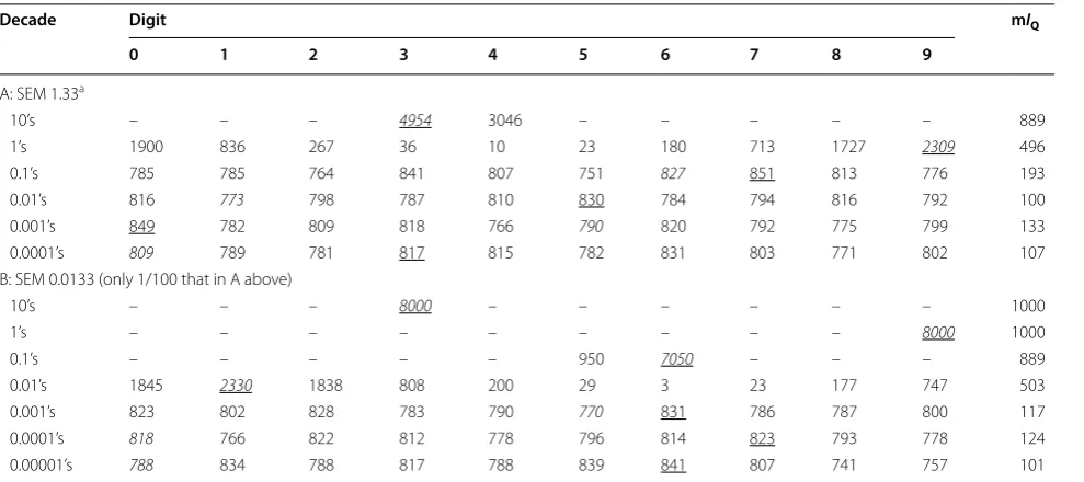
To understand the trends, consider Table 1A which shows the frequency of digits in 6 decades (from the ‘10’s to the ‘0.0001’s) in 8000 random samples from a popula-tion of Gaussian (‘normal’) values with mean 39.61500 and SEM 1.33. In the 10’s decade the frequency of ‘3’s is a bit more than that of the ‘4’s, reflecting the mean of 39…. The influence of the second digit (‘9’) is thus visible in the frequency of ‘4’s in the ‘10’s decade. The count (in italic) in target digit ‘3’ is also the most frequent (underlined). This decade is clearly significant: one or more digits close to the target dominate the frequencies. The same is true of the ‘1’s decade, though here there is a clear pattern of decline in frequency centred around the target ‘9’. In the ‘0.1’s decade the target digit (‘6’) is only next to the most frequent digit (‘7’), and pattern around ‘7’ is not conspicuous.
We may measure inequality (non-uniformity) across the digits in a decade with an index, IQ, based on the sum of absolute deviations from the mean in a row/dec-ade, defined by the ‘R’ expression ‘sum (abs (x − xbar))/s’, where x is a vector of the 10 counts for the individual dig-its, 0–9, xbar is the mean of the ‘x’ values, and ‘s = 2 * (sum
Open Access
(x) − mean (x))’ is a standardisation factor that brings IQ into the range 0–1. In Table 1 the IQ values are multiplied by 1000 as mIQ.
This IQ measure is linear and is a pure number, so val-ues in different decades (rows) can be summed.
In Table 1A there are big reductions in IQ in the first 3 decades; thereafter values differ erratically governed by random frequencies of the digits. This pattern resembles an ice-hockey stick. As you move down the handle (rows/ decades in Table 1A) the downward steps in the inequal-ity measure are large. But when you reach the blade, dif-ferences in the measures between rows/decades become erratically smaller and larger, with no obvious further predictable change with additional rows/decades. At what decade may we suppose that little or no more use-ful information is present? This is tantamount to locating the junction between the hockey stick handle and blade. This is not a sharp angle, but a mIQ value of 200 seems, from Table 1, to be suitable. A crude stopping-rule is thus to continue down the decades until mIQ is below 200, i.e. (Table 1A) to the same decade as the first digit in the SEM. This becomes Rule 1 in Rules Box (later).
This rule uses the SEM to show where to stop: it makes no use whatever of the position of the decimal point. For example, the value 12.345 mm has 5 digits after the first non-‘0’, and 3 decimal places, while the same value in dif-ferent units is 0.012345 m which also has 5 digits after the first non-‘0’ (i.e. ignoring preceding zeros) but 6, not
3, decimal places. Rules-of-thumb that specify a number of decimal places miss the point (literally as well as meta-phorically) that precision is measured by SEM (and n).
Table 1B shows similar results for the same mean as in Table 1A, 39.61500, but SEM 100 times smaller. The same features are visible, and the same crude stopping-rule emerges. The ‘10’s and ‘1’s decades show only a single (the target) digit.; not until the ‘0.1’s do the frequencies begin to spread out.
The IQ calculation takes no notice of the order of the frequencies within a decade. Murray Hannah (personal communication) points out that at least one more decade may contain some residual conditional information. For example, in Table 1A, the 0.1’s decade contains the ‘run’ of increasing or decreasing values 751, 827, 851, 813, 776, draped over the most frequent value: a faint echo of the strong patterns in earlier decades. But in Table 1B at the ‘0.001’s decade (the first with mIQ < 200) there is no sign at all of a sequence. It seems that we need to add some-where between 0 and 1 digits to the sigdig identified by the basic stopping rule (though this would require a frac-tional decade). At worst, the crude rule becomes stop at the same decade as the second digit in the SEM.
A continuous index and trends for sigdigs
In Table 1A counts in the ‘0.1’s decade show little regular-ity, but if we were to decrease the SEM gradually (details not shown) the totals for each digit in a decade become Table 1 Distribution of digits in a sample of 8000 values with mean 39.61500
Values drawn randomly from a Gaussian (‘normal’) population with mean 39.61500 and SEM as shown. The target digit in each decade is in italic; the most frequent digit in each row/decade is underlined. ‘–’ represents ‘0’. The sample of 8000 is an arbitrary choice that gives cell entries (in the lower rows) three digits. One measure of
inequality along a row is IQ (the standardised sum of absolute differences from the row mean, range 0–1, see text), presented here multiplied by 1000 as mIQ
a By the 0.1’s the target digit is not the most frequent
Decade Digit mIQ
0 1 2 3 4 5 6 7 8 9
A: SEM 1.33a
10’s – – – 4954 3046 – – – – – 889
1’s 1900 836 267 36 10 23 180 713 1727 2309 496
0.1’s 785 785 764 841 807 751 827 851 813 776 193
0.01’s 816 773 798 787 810 830 784 794 816 792 100
0.001’s 849 782 809 818 766 790 820 792 775 799 133
0.0001’s 809 789 781 817 815 782 831 803 771 802 107
B: SEM 0.0133 (only 1/100 that in A above)
10’s – – – 8000 – – – – – – 1000
1’s – – – – – – – – – 8000 1000
0.1’s – – – – – 950 7050 – – – 889
0.01’s 1845 2330 1838 808 200 29 3 23 177 747 503
0.001’s 823 802 828 783 790 770 831 786 787 800 117
0.0001’s 818 766 822 812 778 796 814 823 793 778 124
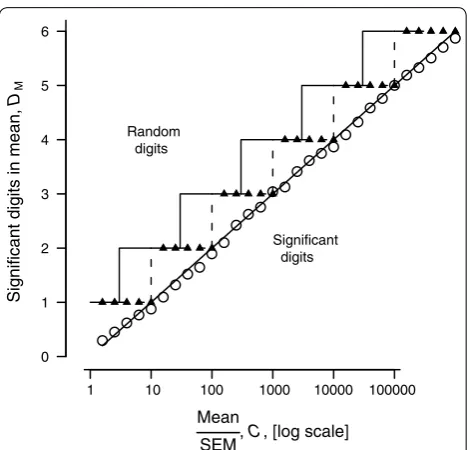
[image:2.595.57.552.100.320.2]more and more unequal as frequency peaks emerge and grow from the hummocky sinking plain and, con-sequently, indicate that we may soon be able to justify another sigdig. The examples in Table 1 are indicative, but to understand the trends and to distil general rules, we need a sigdig index, DM, for the mean that is continu-ous, and which can be plotted on a graph. For this pur-pose, because IQ is linear, we can simply add the IQ values for each decade (row) until we stop at the last decade with mIQ more than 200 (IQ more than 0.2). This value, DM= ΣIQ, is then a plottable measure of sigdigs (Figs. 1 and 2).
In Fig. 1, the large circles are for a stopping rule at 200 mIQ, Putting the stopping rule at 100 mIQ (not shown) makes little difference.
Sigdigs in the SEM, DSEM (Fig. 2) are got in the same way as DM.
Distilling rules
The points in Fig. 1 show how DM depends experimen-tally on C, the quotient of mean/SEM in experiments similar to those outlined in Table 1. The sloping line,
DM= log10 C, is close to the circles, but is not fitted to them. If we take the ceiling of these values—equivalent to truncating and adding 1—to get an integer value we get the broken line in Fig. 1, superimposed on which is the direct integer sigdig (triangles). The overshoot into the random digits region is from 0 to 1 sigdig.
The possibility of Murray Hannah’s contingent infor-mation may be accommodated by adding one extra decade to the dashed steps (Fig. 1). It may be accommo-dated in another way: shift the steps about half a decade left using log10 (3) ≈ 0.5 (continuous line steps in Fig. 1). The overshoot is more uniform at 0.5–1.5 digits, and this accommodates most if not all contingent information.
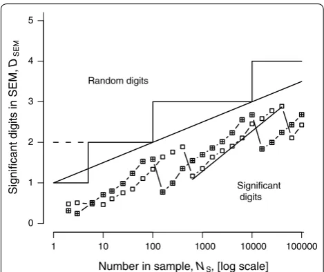
Rule 2 for DSEM is simpler but its origin is more com-plicated. Figure 2 shows, for a fixed mean and standard deviation (SD), how DSEM depends, in experiments simi-lar to those in Table 1, on the number of items, NS, in the calculation of an SEM. Points for two such experiments, with the same mean and different SDs are shown. Over a range of 100 the value of DSEM rises with a slope ≈ 1 on the log-linear scales shown: DSEM≈ log10 (NS) +c, but eventually it falls over a cliff creating a sawtooth pattern. The cliff effect is at first very confusing. We know that the precision of the SD estimate must increase monotoni-cally with increasing sample size. So too must the pre-cision of the SEM. The reason for the cliffs is that, since SEM = SD/√NS, it also decreases in magnitude. With
every 100-fold increase in NS the SEM loses a leading sig-nificant decade, as a ‘1’ in the leading decade shrinks to a ‘9’ in the next decade. So while the precision increases, the number of significant digits decreases by one.
The overall slope of this saw-toothed progression (≈ 0.5) is half that of the teeth themselves reflecting the fact that the SEM depends on √NS. The exact position of the saw-tooth depends on the numerical value of the SEM, and to accommodate this the bounding line DSEM= log10 (NS)/2 + 1 is shown. The steps show Rule 2 in Rules Box. The offset for
NS≤ 6 accommodates the fact that at small NS the bounding line curves downwards, though this is not shown in detail in Fig. 2. Reports of percentages have additional problems. The Rules Box below lists all these rules. Cole [2] considers the special case of risk (and other) ratios (strictly quotients).
Mean
SEM, C, [log scale]
Significant digits in mean,
DM
1 10 100 1000 10000 100000 0
1 2 3 4 5 6
Random digits
Significant digits
Fig. 1 Experimental dependence of sig-digs in a mean, DM, on the
C= mean/SEM quotient. The small triangles are integer significant digits that are the sum of the decades reached so far. The unfilled circles are the index DM. They are close to the line DM= log10 (C) line
(with slope 1.0 and intercept zero). The area below and to the right of this line is the domain of significant digits in the mean; above and to the left the digits are random junk. The broken line staircase above the diagonal DM= log10 (C) line shows the simple case for integer (1,
2, 3 and so on) sig-digs. Rule 1A (in Rules Box, near the end) is for this broken line (see text). The unbroken line staircase shows the better but slightly more complex Rule 1B (listed in Rules Box, near the end) that gives a more uniform distance between the staircase and the
[image:3.595.305.539.85.310.2]Rules Box
Rule 1A: for significant digits (DM) in the mean:
The last significant digit in the mean is in the same decade as the first digit in the SEM; but, better is
Rule 1B
if the first significant digit in C= mean/SEM is ‘4’ to ‘9’ then, as in Rule 1A; but if C is ‘1’ to ‘3’ then the last
significant digit in the mean is in the same decade as the
second digit in the SEM.
Rule 2: for significant digits (DSEM) in the SEM itself:
n in sample 2 to 6 7
to 100 101 to 10,000 10,001 to 1e6 > 1e6
Significant
digits, DSEM 1 2 3 4 5
Rule 3: for counts as percentages
For fewer than 100 observations then two digits in a percentage overstate the precision. For more than 100 (assuming counting statistics) Rule 1 applies.
n in sample* 11
to 20 21 to 50 51 to 100 101 to 10 000 10 001 to 1e6
Report % to the near-est/%
5 2 1 0.1 0.01
*For 10 or fewer observations do not use %
Examples: 7/17 = 40% (not 41.17… %); 6/17 = 35%; LimitationThis analysis deals with precision alone. Bias (and some-times mistakes) may often have a bigger effect on a mean than does precision.
Authors’ contributions
RSC is the sole author. The author read and approved the final manuscript.
Acknowledgements
I thank Murray Hannah for pointing out possible contingent information beyond the DM limit. I salute those whose ignorance of when to stop goaded me to start this work.
Competing interests
RSC declares that he has no competing interests.
Availability of data All in the article.
Consent for publication Not applicable.
Ethics approval and consent to participate Not relevant.
Number in sample, NS, [log scale]
Significant digits in SEM,
DSE
M
1 10 100 1000 10000 100000 0
1 2 3 4 5
Random digits
Significant digits
Fig. 2 Experimental dependence of sig-digs in the SEM, DSEM, on the
SEM sample size, NS. For samples from a Gaussian population of 107
with mean 39.5681 and the arbitrary standard deviation (SD) = 21.60 (empty squares) the points are close to a series of segments of lines DSEM= log10 (NS) + c. The squares with a cross inside show a
similar pattern for a SD half that used for the empty squares. The line through the mean for one sawtooth has a slope of 1.0. The longer sloping line y= log10 (NS)/2 + 1, with half the slope of the sawtooth
lines, summarizes the upper bound of sawtooth lines and sets the boundary between significant and random digits. The staircase ending in a broken line, with a step every 100-fold increase in NS
shows the simplest rule for significant digits in an SEM. The staircase with continuous lines and a short step at the bottom shows Rule 2 in Rules Box, taking account of the difference in behaviour for very small NS
Special cases of zeros
Suppose a raw mean of 0.0298699, has DM= 3 sigdigs under Rule 1A. The reported value should be 0.0300. The first two ‘0’s locate the decade of the first sigdig; the final two ‘0’s are significant, and their presence is sufficient to show that. They should not be omitted.
But suppose that the raw mean is 298,699 with 3 sigdigs again, then the reported value should be 300,000. The first two ‘0’s are sigdigs, but the next 3 function only to show where the decimal point is. One way (there are oth-ers) to indicate such packing digits is by italics: 300,000, or by expressing the value in exponent form: 3.00e5.
[image:4.595.304.539.86.283.2]•fast, convenient online submission
•
thorough peer review by experienced researchers in your field
• rapid publication on acceptance
• support for research data, including large and complex data types
•
gold Open Access which fosters wider collaboration and increased citations maximum visibility for your research: over 100M website views per year
•
At BMC, research is always in progress.
Learn more biomedcentral.com/submissions
Ready to submit your research? Choose BMC and benefit from: Funding
None.
Publisher’s Note
Springer Nature remains neutral with regard to jurisdictional claims in pub-lished maps and institutional affiliations.
Received: 7 December 2018 Accepted: 11 March 2019
References
1. Margolis HS, Barwood GP, Huang G, Klein HA, Lea SN, Szymaniec K, Gill P. Hertz-level measurement of the optical clock frequency in a single 88Sr+ ion. Science. 2004;306:1355–8.