Influence of some environmental factors on CIPA movement into soil

1969

Influence of some environmental factors on CIPA

movement into soil

Myron Paul Molnau

Iowa State University

Follow this and additional works at:

https://lib.dr.iastate.edu/rtd

Part of the

Agriculture Commons

, and the

Bioresource and Agricultural Engineering Commons

This Dissertation is brought to you for free and open access by the Iowa State University Capstones, Theses and Dissertations at Iowa State University Digital Repository. It has been accepted for inclusion in Retrospective Theses and Dissertations by an authorized administrator of Iowa State University Digital Repository. For more information, please contactdigirep@iastate.edu.

Recommended Citation

Molnau, Myron Paul, "Influence of some environmental factors on CIPA movement into soil " (1969).Retrospective Theses and

Dissertations. 4674.

FACTORS ON CIPA MOVEMENT INTO SOIL.

Iowa State University, Ph.D., 1969

Engineering, agricultural

by

Myron Paul Molnau

A Dissertation Submitted to the

Graduate Faculty in Partial Fulfillment of

The Requirements for the Degree of

DOCTOR OF PHILOSOPHY

Major Subject: Water Resources (Agricultural Engineering)

Approved:

f Major Work In Char;

Head of Major Department

Iowa State University

Ames, Iowa

1969

Signature was redacted for privacy.

Signature was redacted for privacy.

Page

I. INTRODUCTION 1

II. OBJECTIVES 2

III. LITERATURE REVIEW 3

A. Herbicides in the Soil 3

1. Movement of pesticides in the soil ^

2. Losses of herbicides from the soil 9

B. Herbicides in Runoff Water 14

C. Extraction and Detection of Herbicides 16

1. Extraction procedures for soils 16

2. Extraction procedures for water and sediments 17

3. Detection of herbicides by gas chromatography 19

IV. EXPERIMENTAL METHOD 24

A. Watershed Experiment 24

1. Description vf the experiment 24

2. Collection of sediment samples 28

3. Collection of soil samples 29

B. Laboratory Experiment 36

1. Description of the experiment 37

2. Equipment and materials 38

C. Preliminary Tests and Results 44

1. Detection of CIPA and general operating procedures 44

2. Extraction of CIPA from soil 54

3. Extraction of CIPA from water 61

TABLE OF CONTENTS (continued)

Page

V. RESULTS AND DISCUSSION 73

A. Laboratory Results and Discussion 73

1. Amount of movement 73

2. Shape of sphere-of-influence 80

B. Observations about Recovery and Degradation 95

1. Recovery of CIPA from the granule and soil 95

2. Observations on degradation 99

C. Watershed Results and Discussion 100

1. Loss of CIPA with time 100

2. Variation of CIPA with location and depth 118

3. CIPA in runoff water and sediment 119

D. Observations on Watershed and Laboratory Results 119

VI. SUMMARY AND CONCLUSIONS 121

VII. SELECTED REFERENCES 124

VIII. ACKNOWLEDGMENTS 130

IX. APPENDIX A. COMPUTER PROGRAM FOR DATA REDUCTION 131

X. APPENDIX B. EXPERIMENTAL DATA 149

A. Calculated Data 149

B. Computer Output 157

1. Laboratory data 157

One of the major problems facing the food producer today is the

decrease in production due to weed competition with crops. The control of

these losses with minimum cost and maximum control involves increasing

amounts cf selective and general purpose herbicides. These herbicides

must all be absorbed within the environment in either a degraded or the

original form. Both the popular and technical press have expressed concern

about the effects of these herbicides, and agricultural chemicals in

general, on our environment. This concern is being voiced because the

ultimate fate of these agricultural chemicals and their effect on the

general ecosystem is not completely known.

The use of herbicides should be governed by the idea that their most

efficient use is one that gives maximum weed control with a minimum

contamination of soil and water. Such usage implies both accurate

placement and dosage. A granular formulation is one method of achieving

the accuracy required in placement and dosage of the herbicide.

Many obstacles lie in the path of ideal use of herbicides in granular

form. Two of the most pressing are the dosage necessary to kill weeds

under varying conditions is not known, and the factors governing the

movement of herbicides from granules into the soil are poorly understood.

When the underlying principles regarding the movement of herbicides

in the soil are better understood, the engineer will be better able to

design machinery for more precise granule placement, and farmers will be

better able to choose the proper weather and soil conditions to maximize

II. OBJECTIVES

The overall objective of this study was to obtain a better understand­

ing of herbicide movement in soil. Specific objectives were as follows:

1. To describe the influence of initial soil moisture content,

relative humidity of the air above the soil, environmental temperature,

and depth of incorporation on the shape and size of the soil volume into

which herbicides move from granules.

2. To describe the effects of initial soil moisture content, relative

humidity of air above the soil, environmental temperature, and depth of

incorporation on the losses of herbicides from the soil.

3. To develop methods and techniques of sampling and measuring the

concentration of herbicides in soil and runoff following application to

controlled watersheds.

4. To describe the spatial and temporal distribution of a herbicide

The vast amount of literature on the general subject of herbicides

made it imperative that some logical sequence be followed in reading the

literature. The literature on herbicides was divided into herbicides in

the soil, herbicides in runoff water, and detection and extraction of

herbicides from soil and water.

During the past three years several symposiums have been held and

which have published proceedings (American Chemical Society, 1966; Soil

Science Society of America, 1966; Brady, 1967). These proved to be very

valuable and will be extensively cited. The American Chemical Society also

periodically publishes literature reviews on the analytical aspects of

pesticides which were very valuable (Cook, 1965; Williams, 1967; Westlake,

1957, 1959, 1961, 1963; St. John, 1953, 1955).

A. Herbicides in the Soil

A large body of literature exists describing the behavior of specific

herbicides when applied to the soil. Individual papers are usually about

one herbicide or class of herbicides such as the triazines or ureas and

not about the characteristics of all herbicides. Specific information was

sought on 2-chloro-N-isopropylacetanilide (CIPA), the anilides and amides,

and compounds which could be expected to behave as the anilides because of

their structure, such as the ureas and carbamates.

Herbicides in the soil may be reviewed by looking first at their

movement in the soil and then at losses of herbicides from the soil. The

end of this chapter in Table 1.

1. Movement of pesticides in the soil

A general theory of movement of nutrients in the soil has been

proposed (Barber, 1962). He proposed that nutrients reach a plant root

by mass flow, diffusion, and interception. Mass flow occurs when ions

move with the soil water to the root. If the root is able to absorb the

ions at a rate greater than the ion transport rate, no ions will

accumulate at the root-soil interface. Conversely, if the uptake rate is

less than the transport rate, the ions will accumulate at the interface.

Diffusion through the soil water will occur when the uptake rate is

greater than the mass flow transport rate. The third means of obtaining

nutrients is by root interception where the roots reach the nutrients by

touching and removing the ions attached to soil particles.

Barber's theory of nutrient movement was applied to herbicides by

Lavy (1968) who studied the s-triazines. He found that for a silty clay

loam, atrazine and propazine moved by mass flow while simazine moved to

the root by diffusion. With a sandy loam, atrazine moved by mass flow,

simazine by diffusion but no movement was observed for propazine. This

agrees, in general, with the solubility of these compounds of which

atrazine is the most soluble and simazine the least. The radio-carbon

method of measurement did not allow measurement of movement by soil air

diffusion.

Cearlock (1966) approached the movement of pollutants in the soil

from a transport theory point of view. He visualized total movement as

diffusion and dispersion. The concentration at any point was then the

result of these two mechanisms plus the interaction of biological,

chemical, and physical reactions.

The vast number of papers dealing with leaching and adsorption of

pesticides is evidence that many researchers feel these are the most

important properties influencing herbicide movement. Harris and Warren

(1964) determined the adsorption and desorption characteristics of CPIC,

DNBP, diquat, atrazine, and monuron. CIPC was more strongly adsorbed by

anion than cation exchangers, and only moderately affected by pH. Monuron

showed similar characteristics but less was adsorbed. The amount adsorbed

showed a strong temperature dependence with monuron having 47 percent

adsorbed at 0 C and 8 percent at 50 C.

Adding 0.25 inch increments of water by subirrigation resulted in

greater movement of dicamba and diphenamid than if one inch increments

were added (Harris, 1964). Harris (1966) also showed that adsorption of

monuron was weakest for a sandy loam and strongest for a silty clay loam.

Lambert and others (1965) developed an unusual method for obtaining

data on chemical movement in the soil. According to their results the

Gaussian equation could be used to describe movement of a chemical caused

by water percolation in soil columns. The equation is based on the

assumption that soil is much like a chromatographic column consisting of

an inert support (mineral particles) and an organic phase, a water phase,

coefficient, they calculated the movement of an herbicide due to percola­

ting water.

Herr and others (1966) studied the movement of picloram under field

conditions. Plots were sampled in six inch increments to three feet.

Surface application rates of 2, 4, 8, 32, and 64 oz/acre were used.

Regardless of soil type or rainfall, the highest concentrations were in

the top six inches three months after application. After eight months,

some picloram was found distributed through the entire profile for two

samples and to a depth of two feet for another. The highest concentrations

were in the top six inches for a heavy and a medium-textured soil but at

the deepest sampling depth for a light-textured silt loam. After 15

months, some picloram was detected at all application rates on a plot

with low rainfall and heavy-textured soil. None was found in the sampled

profile of a light-textured soil for the 2, 4, and 8 oz/acre applications.

However, the highest concentrations were again at the deepest sample

depths for the 32 and 64 oz/acre application rates. The medium-textured

soil also had no residues for the low rates but showed a uniform profile

distribution of picloram to three feet. They concluded that soil organic

matter was the most important factor in retaining picloram from leaching.

Keys and Friesen (1968) indicated that most of the picloram remained

in the top six inches regardless of application rate but that greater

downward movement occurred in low organic matter soils. All four soils

were loams and received rainfall of 22.9 inches in 23 months.

Harris and Sheets (1965) studied the chemical and physical

properties of soil and the amount of herbicide adsorbed from an aqueous

inhibition of oat seedling growth when diuron and simazine were used.

Organic matter content correlated best with seedling growth for CIPC.

None of the easily measured soil properties (field capacity, organic

matter, cation exchange capacity) provided consistent predictors of dosage

effects on the oat seedlings.

McGlamery and Slife (1966) studied atrazine adsorption on a Drummer

clay loam. They found that adsorption by the soil increased as pH

decreased and that concentration of atrazine and temperature had little

effect. Desorption increased with temperature and pH. Talbert and

Fletchall (1965) found that the increasing adsorption order for the

triazines was propazine, atrazine, simazine, prometone, and prometryne.

Organic materials generally adsorbed more than the clays.

Anderson and others (1968) reported on the leaching of nitralin,

benefin, and trifluralin in soil columns. All three herbicides had the

same solubility in water but nitralin was leached far more easily than the

others from a clay loam. Nitralin was leached four inches by four inches

of water and 4.5 inches by ten inches of water. Benefin was not leached

past the 2.5 inch depth while trifluralin was not leached past 3.5 inches.

Rogers (1968), in studying the leaching of seven s-triazines,

observed that factors other than solubility affect leaching of herbicides.

In decreasing order of leachability, the s-triazines studied were

atratone, propazine, atrazine, simazine, ipazine, ametryne, and prometryne.

This agrees with the order of adsorption on soil found by Talbert and

solubility in adsorption studies.

Baily and White (1964) have published the most comprehensive review

of adsorption and desorption to date. A total of 161 references, which

were published prior to April 1963, were cited. This review covered the

role of soil or colloid type, physico-chemical nature of the pesticide,

soil reactions, type of cation on the colloid exchange site, soil moisture

content, nature of formulation, and temperature. It was determined from

the review that the physical properties of the soil exerted only an

indirect influence on adsorption. In general, it was found that the

activity of pesticides towards biological systems was lowest in soils

which were high in organic matter and clay content, with organic matter

being the more important of the two, and highest in sandy and loamy soils.

Leaching was found to be influenced by the solubility of the pesticide

and adsorption of the pesticide onto soil particles. Most authors

reported that solubility and temperature work together to decrease adsorp­

tion as temperature rises. EPTC was an exception which had the greatest

adsorption at the highest temperature. There was general agreement that

there was greater vapor loss due to increased temperature for DNBP, EPTC,

CDEC, and CDAA. Low soil moisture was characterized as favoring adsorp­

tion, while high moisture favored lower adsorption and greater movement.

Mullins (1965) studied the micromovement of CDAA from a granule into

soil. He investigated the influence of initial soil moisture, air move­

ment, and surface applied water on the CDAA distribution. The movement

which was noted appeared to be the result of either gaseous diffusion or

of water vapor acting as a vehicle for transporting CDAA. For incorporated

One feature noticed by Mulling is the bulb-shaped sphere-of-influence

of the incorporated granule in air dry soil. The herbicide from the

granule moved mainly downward and laterally in air dry soil rather than

upwards as in soil at field capacity. Thus it appears that for dry soils,

incorporation would put the herbicide below the layer where weed seeds

germinate. Siegel and others (1951) found that for two fumigants, this

same sort of dispersion pattern holds, i.e., movement was downward and

lateral with little if any movement upward. Moisture content made no

difference in this pattern but more movement was noted for a soil at the

moisture equivalent than air dry.

2. losses of herbicides from the soil

The factors which influence the disappearance of a pesticide from

the soil can be divided into the three general groups of environmental,

metabolic, and physical factors (Van Middelem, 1966). Environmental

factors listed were climate, soil type, plant type, microorganisms, and

animals. Metabolic factors included molecular alterations and transport

mechanisms in plants and animals. Physical factors included growth

characteristics of the plant or animal and the climatic parameters such as

light, relative humidity, temperature, and so forth.

One of the reasons for the continuing search for specific short­

lived pesticides has been the concern about the biological consequences of

buildup of residues in soils. Hamaker (1966) proposed several mathemati­

cal models for predicting long term residue buildups in the soil. The

degradation model (the decay rate is proportional to the amount present).

He found that the residue present immediately after addition of the annual

increment, r, was a function of the fraction left after one year, f, and

the initial concentration, C^. The expression is

(^L = i/(i-f) o

For this case, the maximum accumulated residue for a half-life of three

months was 1.07 times the annual increment. For a half-life of one year,

the accumulation was twice the annual increment and for two years, the

accumulation was 3.40 times the annual increment. In studies in which

this first order law was applied to aldrin and dieldrin, Lichtenstein

and Schulz (1965) found the half-life of aldrin to be 4.2 years for

Illinois soils with a 24 percent conversion efficiency of aldrin to

dieldrin. Hamaker used this data to calculate dieldrin residues for a

five year period. The analysis of field samples showed 2.0 ppm and the

calculated result was 2.4 ppm. The field results and calculated results

agree exactly at two years, indicating that for Illinois conditions,

dieldrin degradation was approximately a first order reaction. Degradation

predicted by mathematical models is a descriptive device only. Nothing is

said about the factors that influence disappearance from the soil.

Some of the processes which result in losses of pesticides from soils

are volatilization, catalytic decomposition, photoinactivation, irreversi­

ble adsorption, microbial decomposition, leaching, and plant uptake (Gray,

1965; Lambert and others, 1965). Two factors which have had extensive

actually went down with increasing temperature as relative humidity was

reduced. It was also found that volatility losses were higher at low soil

moisture contents and high temperatures.

Mullins (1965) found that CDAA granules observed 48 hours after

being placed on a soil surface initially at field capacity lost four times

as much CDAA by volatilization as had granules on an air dry soil surface.

Losses by vaporization and air movement were less for incorporated granules

than for surface applied granules.

Parochetti and Warren (1966) investigated the vapor losses of IPC and

CIPC from a soil surface as influenced by temperature, soil moisture, soil

type, air flow rate, and formulation. A direct trap was used to catch all

vapor leaving the soil surface. They found that IPC was more volatile than

CIPC. CIPC losses increased by 50 percent when air flow rate over the

soil went from two to six cubic feet per hour and also losses increased

from almost nothing to 35 percent as temperature increased from 20 to 45 C

on a quartz sand. Temperature had little effect in an air dry silt loam,

however, at field capacity the CIPC losses increased with temperature while

IPC losses increased and then decreased as temperature was raised. Losses

due to volatilization decreased as percent organic matter and clay content

increased and as moisture content decreased. They also reported that IPC

losses were lower from spray applications than granules but no difference

could be noted for CIPC. Covering IPC with 1/8 to 1/4 inch soil reduced

losses by half on a silt loam and by a fourth on sand, while CIPC losses

on the disappearance of CDEC from a soil surface. He found the same loss

of CDEC occurred on a sandy clay loam as on a loamy sand. Relative

humidity had no effect on the loss. Temperature and soil moisture were

found to be the most important of the parameters studied.

Gray (1965) reported that much less EPTC was lost from dry soils than

moist. Incorporating EPTC immediately after application prevented all

loss from the dry soils and greatly reduced the loss from moist soils.

In another study. Gray and Weierich (1965) showed that the moisture

content of the soil was the most important factor related to vapor loss

of EPTC. For spray applications, the losses after one day were 23, 49,

and 69 percent from dry, moist, and wet soil, respectively, and 44, 68,

and 90 percent after six days. For granular application, there was no

loss from soil for the first ten hours in soil below six percent moixture,

but at 15 percent moisture, the loss was 60 percent in two hours. There

was a critical moisture content above which large losses could be

expected. Depth of incorporation was found to be very important also.

A depth of two to three inches was needed to prevent losses after light

rain or sprinkling.

If the pesticide disappears from the soil but is not lost by

volatilization, the disappearance is most likely due to decomposition of

the pesticide, which may be either chemical or microbial. Kaufman and

others (1968) found that amitrole degraded mainly by chemical rather than

microbial means. Several soil types and different means of sterilization

were used. They voiced concern that just because autoclaved soil showed

who cautioned that the method of sterilization may induce some changes

in the soil environment. The possibility also arises that changes in the

soil brought about by microorganisms may cause decomposition. In this

case the microorganisms would be an indirect cause of degradation.

Bartha and others (1967) and Bartha and Pramer (1967) studied the

effect of 29 different pesticides on CO^ production from soil. Four of

these compounds are of interest, diphenamid, karsil, stam F-34 (propanil),

and dicryl. Concentrations used were well above normal field applications

(over 200 ppm). The results showed an initial increase in CO^ production

followed by a decrease. One of the hydrolysis products of propanil was

toxic to the microorganisms. This toxicity increased over a 30 day

period.

It was also shown that dicryl, diphenamid, and karsil inhibited

nitrification for a period of 30 days. The three anilides caused a strong

and lengthy inhibition of nitrification and influenced the soil nitrifica­

tion. It was postulated that the increase in COg production indicated the

compounds degraded and the organisms used them as a source of carbon. In

a later test, Bartha (1968) used CIPA as well as propanil, dicryl, and

karsil. He found the microbes oxidized the carbon on the aliphatic side

chain. CIPA was the least subject to microbial degradation of these

chemicals and after 21 days, 90 percent of the applied amount was still

present although a much greater inhibition of respiration occurred with

CIPA than with other compounds. This was due to the herbicide itself

application rates were 200 ppm in the soil which is well above the normal

agricultural application of 1 to 3 ppm.

In an investigation on the phytotoxicity of some phenylureas. Comes

and Tinmons (1965) found that diuron, monuron, and fenuron activity was

materially decreased when exposed to sunlight on a soil surface for 25

days and temperatures were below 120 F. They reported that temperature

and air movement had to be carefully controlled to separate the various

decomposition effects from photodecomposition. Danielson and Centner

(1964) also reported on air movement influences in the loss of EPTC. They

found that there was an inverse relation between air velocity and EPTC

persistence but that soil composition and spray formulation did have a

modifying effect.

B. Herbicides in Runoff Water

Much concern has been expressed about the effects of agricultural

chemicals in runoff from agricultural lands, particularly insecticides and

herbicides (Pope and others, 1966; Sparr and others, 1966; Van Valin,

1966; Barthel and others, 1966; Quigley, 1967; Green and others, 1967;

Iverson, 1967). Much of this effect has been directed towards the

chlorinated hydrocarbon insecticides because of their persistence and

toxicity.

Sparr and others (1966) studied endrin and aldrin in runoff from

cotton fields and found concentrations of 50 ppt of endrin in water but

none in mud and traces in fish. As reported by Van Valin (1966), a

water within two weeks, while vegetation and soil samples showed the

highest residue level within two days. Wettable powder application

produced the highest level in water and fish within three days.

Parathion, an organophosphate, was found to persist for 96 hours after

application with irrigation water. The reported concentrations were

toxic to some aquatic organisms (Miller and others, 1967).

Crop rotation has been found to have an effect on the pesticides in

runoff. Trichell and others (1968) reported that 24 hours after applica­

tion, losses of dicamba and 2,4,5-T was greater from sod than from

fallow plots that received simulated rainfall. Picloram losses were the

same for both plots. Bamett and others (1967) reported that 2,4-D in

runoff from cultivated fallow land was positively correlated with the

amount applied to the soil. The highest concentrations were found early

in the storm. Water temperature had a positive influence on the concen­

tration in the water. Epstein and Grant (1968) reported that the

concentration of DDT, endrin, and endosulfan was lower in runoff from

plots in a potato, oats, sod rotation than from continuous potato plots.

More pesticide was found in the soil-water suspension than in the

settled muds.

Frank and others (1967) studied fenac and dichlobenil in irrigation

water. These herbicides were used to control weed growth in canals between

irrigation seasons. It was found that the first water flowing over the

treated areas contained concentrations of 8.7 ppm (enough to damage crops).

C. Extraction and Detection of Herbicides

The choice of a method to extract the herbicide from soil and water,

and detect the herbicide with the desired sensitivity was greatly

facilitated by several manuals dealing with residue analysis.

Burchfield and Johnson (1965) have compiled a guide for the use of

research workers while the Department of Health, Education, and Welfare

(1968) has published a manual intended for use in law enforcement. One

volume of a four volume work edited by Zweig (1964) covers a few herbi­

cides. Two books dealing mainly with the instrumental aspects of gas

chromatography in the detection of pesticide residues are by Bonelli

(1966) and Gudzinowicz (1965). A good general reference on gas

chromatography is that of Ettre and Zlatkis (1967). These sources provide,

in general, a starting point for the investigation of various extraction

procedures and detection methods for pesticides and CIPA in particular.

1. Extraction procedures for soils

The extraction of a substance from the soil is not as difficult as

from a crop because the fats, oils, and waxes are not usually present in

soil. Thus, pesticides can usually be extracted fairly easily. In most

cases mixing the solvent and soil and either shaking or using a soxhlet

extractor will suffice.

Mullins (1965) used three solvents for shaking extraction of CDAA;

benzene, acetone, and 4:1 hexane-benzene. Soil samples of about one gram

were spiked with CDAA, two milliliters of solvent were added, and the

mixture shaken for varying lengths of time. The results showed that

acetone. Ten minutes also proved to be optimum shaking time.

The literature is replete with soil extraction procedures. Almost

all references cited in previous sections give extraction procedures.

Suffice it to say that, in general, compounds of similar structure may or

may not behave the same and that the best procedure will be found by

experimenting with the various procedures listed in the pesticide manuals.

The Department of Health, Education, and Welfare (1968) suggests the use

of acetonitrile for use in extracting CIPA from various crops.

Solvents which have been used are chloroform for CDEC (Taylorson,

1966), hexane for chlorinated insecticides (Bowman and others, 1965),

acidified acetone for picloram (Merkle and others, 1966), and acetone for

DCA (Bartha and Pramer, 1967). The Health, Education, and Welfare manual

(1968) provides many choices of solvents but a "universal solvent" for

most pesticides is acetonitrile. Extraction is followed by various parti­

tion procedures. Volume II of that manual gives many specific procedures

for individual compounds. Again acetonitrile is usually used but

petroleum ether and various alcohols are also mentioned. This discussion

can be summed up by a quote from Burchfield and Johnson (p. II (1), 1965):

Presently there is no single sequence of extraction and clean­ up methods which is applicable to the recovery of all

pesticides .... Therefore it is essential that recoveries

of standard compounds be determined for each procedure used

2. Extraction procedures for water and sediments

Extraction procedures for removing pesticides from water samples is

are usually fewer interferences and the choice of solvents is limited.

Almost any pesticide will have a preference for the organic solvent phase

of a water-organic solvent mixture.

Several United States Government agencies routinely analyze the

nation's streams for traces of pesticides and have developed routine

methods for extraction. Lamar, Goerlitz, and Law (1965) presented a

method whereby extraction was done-~dn a separatory funnel using about one

liter of water and 25 milliliters of hexane. Breidenbach and others

(1966) used about 850 milliliters of water sample and 50 milliliters of

9:1 hexane-benzene when using the semi-automatic method of Kawahara and

others (1967). When a separatory funnel was used, the sample was

extracted successively with 100, 50, 50, 50, and 50 milliliters of

hexane. Sediment samples were air dried for three or four days, ground

in a mortar and extracted in a soxhlet for eight hours with a 9:1 hexane

acetone mixture.

Kawahara and others (1967) reported on the use of several solvents

for extraction of endrin and dieldrin. Recoveries of 62 percent for both

pesticides were found when hexane was used as the solvent and 95 and 78

percent for dieldrin and endrin respectively when a mixture of 4 percent

benzene in hexane was used.

A semi-automatic extraction method was compared with hand extraction

in a separatory funnel. Two solvent systems, benzene-hexane and

ether-hexane, were used. Semi-automatic extractions with benzene-hexane were

more consistent as shown by a standard deviation of 4.6 percent versus

8.6 percent for hand extractions. The average recovery of aldrin for the

Burchfield and Johnson (1965) discussed two methods for water

extraction. First, a batch method using a separatory funnel and chloro­

form extraction and second, a continuous extraction method, proposed by

Kahn and Wayman (1964), using petroleum ether. Johnson and Stansbury

(1965) use methylene chloride to extract carbaryl. Faust and Suffet

(1966) presented a comprehensive review of the literature prior to 1965.

A perusal of this review indicated a very wide range of solvents. However,

no papers were found giving extraction procedures for amides or anilides.

The general procedure was to try various solvent systems and select the

best one.

3. Detection of herbicides by gas chromatography

Three types of detection systems are in common use for detecting

herbicides with gas chromatography. These are the microcoulometric, flame

ionization, and electron capture detectors.

The microcoulometric detector is widely used where it is desired to

detect organic compounds which contain phosphorous, halogen, or sulfur

(Burchfield and Johnson, p. V. A. (2), 1965). The desired element is

oxidized or reduced in a furnace and passed to an automatic titration

cell. This system has two advantages over other detectors; it is very

specific and the amount of material chromatographed can be calculated

directly from the chromatogram, eliminating the need for frequent calibra­

tions. A disadvantage of this detector is the $8500 minimum cost.

A flame ionization detector measures the change in a current of ions

flame, the compound is ionized and a change in current is produced. The

flame ionization detector is inexpensive (about $2500), and easy to

maintain and use. It is not a specific detector nor very sensitive and

for these reasons is not as widely used as the electron-capture detector.

A modification of this detector makes it specific for phosphorous.

The electron-capture detector is the most widely used detector in r

pesticide residue analysis. This detector measures the affinity of

compounds for free electrons (Bonelli, 1966).

The source of the free electrons is usually a radio-active substance

such as tritium or radium. As the compound passes through the detector,

a loss of current is measured due to the capture of electrons by the

compound. The cost of this detector compares well with the cost of the

flame ionization detector. It gives a high response for halogen containing

compounds and is insensitive to nonpolar organic compounds.

Trichell and others (1968) used a six foot glass column of 10 percent

DC-200 on 100/200 mesh Gas Chrom Q with an electron capture detector for

dicamba, 2,4,5-T, and picloram. Bartha (1968) used a 1.8 meter stainless

steel column with 5 percent UC-W98 on Chromosorb W with a flame ionization

detector for CIPA, DCA, propanil, and other anilides.

CIPA can be analyzed with a flame ionization detector and a four foot

column packed with 80/100 mesh Diatoport S coated with 3.8 percent SE-30

(Department of Health, Education, and Welfare, 1968). The CIPA was first

converted to N-isopropylaniline while Bartha detected CIPA directly.

Bonelli (1966) recommends the use of two different columns to cover

column. Bonelli has compiled many practical hints on the use of the gas

chromatograph in pesticide analysis. Burchfield and Johnson (1965)

recommend 10 percent DC-200 on 80/90 mesh Anakrom ABS in a six foot glass

column and also a QF-1 and SE-30 mixture on the same support for general

use in residue analysis.

Mullins (1965) detected CDAA directly using five foot stainless steel

columns filled with 15 percent SE-30 on acid-washed Chromosorb W. He

noted that the peaks tailed and that the minimum detectable amount was on

Table 1. Chemical and common names for pesticides mentioned in the literature review

Common name Chemical name

Aldrin Ametryne Amitrole Atratone Atrazine Benefin Carbaryl CDAA CDEC CIPA EIPC DCA DDT Dicamba Dichlorobenil Dicryl Dieldrin Diphenamid Diquat Diuron 1,2,3,4,10,10-hexachloro-l,4,4a-5,8,8a-hexahydro-endo-l, 4-exo-5,8-dimethanonaphthalene 2-(ethylamino)-4-(isopropylamino)-6-Cinethylthio)-s-triazine 3-amino-s-triazole 2-(ethylamino)-4-(isopropylamino)-6-methoxy-s-triazine 2-chloro-4-(ethylamino)-6-(isopropylamino)-s-triazine

N-butyl-N-ethyl-o<, , c.<-trifluoro-2,6-dinitro-p-toluidine

1-naphthyl-N-methyl carbamate N, N-diallyl-2-chloroacetamide 2-chloroallyl diethyldithiocarbamate 2-chloro-N-isopropyl acetanilide Isopropyl m-chlorocarbanilate 3,4-dichloroaniline

2,2 bis (p-chlorophenyl)-l,l,l-trichloroethane

3,6-dichloro-o-anisic acid 2.6-dichlorobenzonitrile 3',4'-dichloro-2-methylacrylanilide 1,2,3,4,10,lO-hexachloro-exo-6,7-epoxy-l,4,4a,5,6,7,8,8a-octahydro-1,4-endo,exo-5,8-dimethanonaphthalene N, N-dimethyl-2,2-diphenylacetamide

6.7-dihydrodipyrido [l,2-a:2',l'-c] pyrazidiinium salts

Common

0, 0-diethyl 0-p-nitrophenyl phosphorothioate

4-amino-3,5,6-trichloropicolinic acid 2,4-bis(isopropylamino)-6-methoxy-s-triazine 2,4-bis(isopropylamino)-6-(methyIthio)-s-triazine 3',4'-dichloropropionanilide 2-chloro-4,6-bis(isopropylamino)-s-trizine 2-chloro-4,6-bis(ethylamino)-s-triazine

c<, o<, o{, trifluoro-2,6-dinitro-N, N-dipropyl-p-toluidine

(2,4-dichlorophenoxy) acetic acid

IV. EXPERIMENTAL METHOD

This study was divided into a watershed experiment and a laboratory

experiment. In order to determine some of the details for each of these,

some preliminary tests and planning had to be performed. Each experiment

will be discussed separately.

A. Watershed Experiment

The watershed experiment can be explained by describing the experi­

mental site, the collection of the runoff water and sediment samples, and

the collection of the soil samples.

1. Description of the experiment

The experiment was conducted on the Gingles Watersheds near the

Western Iowa Experimental Farm at Castana, Iowa. There are six watersheds

ranging in size from 1.3 to 3.8 acres. The soils on the watersheds are

Ida and Monona silt loams.

Two of these watersheds were used for the CIPA study. These are

referred to as the northeast and southwest watersheds because of their

location in the overall experimental area. Figure 1 shows all six water­

sheds with generalized contours sketched in. Figure 2 is a map of the

northeast watershed showing the soil sampling stations superimposed on the

contours, and also a listing of the cultural practices for the 1967 and

1968 sampling periods. Figure 3 is the same type of map for the

southwest watershed.

Contours are on an arbitrary datum

N) Ln

3 acres

May 13 disked and harrowed 16 planted corn

22 sprayed CIPA, 4 lb/acre June 13 sampled soil for CIPA

1968

Apr. 24 disked stalks and plowed 29 disked and harrowed 30 planted corn

May 1 sprayed CIPA, 4 lb/acre

1 sampled soil for CIPA

8 sampled soil for CIPA 14 sampled soil for CIPA 23 sampled soil for CIPA June 3 rotary hoed

6 sampled soil for CIPA

Notes :

O water table well \/ H flume

V rain gage

O sampling location

Map not drawn to scale

Contours are on an arbitrary datum

O

O

O 17

15C 14f

13/

N) o\

0

Figure 2. Sampling locations and cultural practices on the

22 sprayed CIPA, 4 lb per acre

June 13 sampled soil for CIPA 29 formed ridges

1968

Apr . 9 chopped stalks

30 planted corn

May 1 sprayed CIPA, 4 lb

per acre

1 sampled soil for CIPA

8 sampled soil for CIPA 14 sampled soil for CIPA

23 sampled soil for CIPA June 3 sprayed 2,4-D

6 sampled soil for CIPA

18 rebuilt ridges Notes :

© water table well H flume

rain gage

sampling location

not drawn to scale

\ / V

o

Map

Contours are on an arbitrary datum

Figure 3. Sampling locations and cultural practices on the

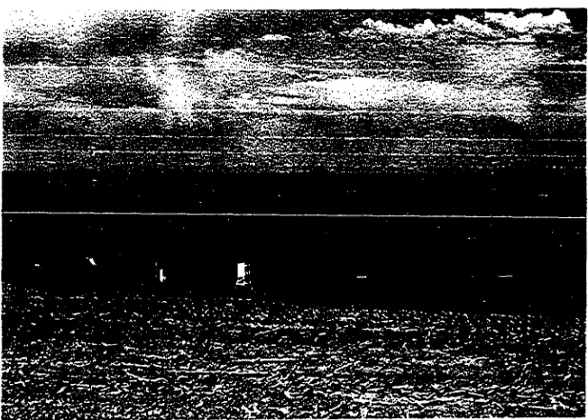
southwest watershed is com planted on contoured ridges. Figure 4 is an

overall view of the southwest watershed, while Figure 5 shows what the

ridges looked like before planting.

The general procedure followed was to apply the CIPA at the rate of

four pounds active ingredient per acre in a spray formulation. The

soil was sampled to various depths at various times. Sampling was

continued until all the CIPA had degraded. During this period, water

runoff was also sampled to determine the amount of CIPA in runoff.

2. Collection of sediment samples

Quantitative sediment samples were obtained from runoff on both

watersheds by single-stage samplers (Figure 6). The sampler is tapped

into the side of the flume (Figure 7) with 3/8 inch copper tubing through

the side of the flume and through the rubber stopper on the bottle. The

one liter sample bottles were of polyethylene in 1967 but were changed to

standard glass one quart milk bottles in 1968.

The single-stage sampler will sample the runoff when the stage reaches

the highest point on the invert of the intake nozzle. This initiates

siphon action and the bottle fills in approximately 20 seconds. Some

trouble was encountered with fine trash and sediment clogging the nozzles.

This was minimized by eliminating the invert. A 1/2 inch intake nozzle

would have helped eliminate clogging.

Qualitative sediment samples were obtained from the southwest water­

shed by use of a two foot Coshocton runoff sampler (Parsons, 1954) (Figure

8). The sampler was offset mounted with the flume centerline at the

was taken. After the water had been collected by the sampler, it would

run to a 55 gallon drum, which contained two small pails of 20 and 5

gallon capacity (Figure 9).

Laboratory tests showed that the offset of the sampler resulted in a

sampling percentage of 0.15 percent for flows less than one cubic foot

per second (cfs) and 0.23 percent for a flow of two cfs. Flows higher

than this could not be obtained in the laboratory. This was not of great

concern because few storms exceed two cfs for any length of time.

In 1967, the samples from the polyethylene bottles were poured into

plastic freezer bags and frozen. Prior to analysis, the entire sample was

weighed and allowed to thaw. The water was removed for separate analysis

and the sediment allowed to dry to a thick paste according to the method

of Breidenbach and others (1966). The paste was weighed, sampled for

moisture, and part of the remainder used for residue analysis. From these

data, both the sediment and CIPA concentration in the sample could be

calculated.

The same procedure was to be followed in 1968 except the samples were

to be frozen in plastic freezer boxes rather than bags. No runoff occurred

during the 1968 sampling period so no comparison of the two methods could

be made.

3. Collection of soil samples

Soil samples were taken with a probe 3/4 inch in diameter. Six cores

were taken transverse to the corn row and composited into a single sample.

Figure 4. View of the watershed

Figure 5. View of the north-middle watershed showing the ridges' before

sample depths of 0 to 1, 1 to 3, and 3 to 5 inches were used until June 6

when the sample depths were 0 to 2, 2 to 4, and 4 to 6 inches. Samples

were collected in standard soil sample bags and frozen immediately after

collection.

Before field sampling could begin, a system for locating sampling

points was chosen. Merkle and others (1966) used 22 by 95 and 22 by 200

foot plots, each of which was sampled in four locations and sampled at the

0-2, 5-7, 11-13, and 23-25 inch depths. The four samples were composited

for analysis. Sikka and Davis (1966) used plots of 5 by 20 feet which they

sampled randomly at six locations at the 0-6 inch depth. The six samples

were composited for analysis. Herr and others (1966) used 20 by 30 foot

plots and also sampled in six inch depth increments. He did not mention

how many locations within each plot were sampled. Nothing was found

regarding sampling of larger fields.

From the standpoint of having a reasonable number of samples to

analyze and still obtain an idea of how much herbicide was applied to the

field, the 125 foot grid spacing was selected. A grid sheet was tossed on

top of a map and the sample points located. Figures 2 and 3 show the loca­

tions of the sampling stations.

B. Laboratory Experiment

The laboratory experiment was set up to determine the effect of

temperature, soil moisture content, relative humidity, and placement on the

In order to carry out the above objective, an experiment was

designed with four different moisture levels, two humidity levels, three

temperatures, and three depths of incorporation.

The moisture levels chosen were air dry (about 3 percent), wilting

point (7.6 percent), field capacity (24 percent), and one point between

field capacity and the wilting point.

A low humidity was chosen to represent an extreme in field condi­

tions and a high value was chosen to represent the high extreme in the

field. The values desired were 20-30 percent and 85-95 percent.

Temperatures were chosen to represent extreme and average conditions.

The temperatures chosen were 50, 80, and 120 F. Table 2 shows that these

were not unreasonable temperatures for the period of the 1968 field

experiment.

Table 2. Temperature data from the Western Iowa Experimental Farm during the 1968 field experiment

Air temperature Soil temperature at one inch

Date Mean Mean Mean Mean

maximum minimum maximum minimum

April 21-30 64 38 63 46

May 1-10 70 44 72 54

May 11-20 67 42 73 52

May 21-30 68 42 73 55

Granules were placed on the surface and at the 1/2 inch depth.

Because a one inch depth was considered extreme, only one test was made

at the one inch depth for each temperature.

2. Equipment and materials

The main items of equipment used were the gas chromatograph, soil

core sampling apparatus, and the humidity chambers.

A Varian Aerograph 660 gas chromatograph was used with an

electron-capture detector. The source is a 150 millicurrie tritium foil.

Prepurified nitrogen was used as the carrier gas. The output signal was

recorded with a one millivolt one second full scale Westronics recorder;

Figure 10 shows the arrangement of the chromatograph, recorder, and

column oven temperature controller.

The soil core sampling apparatus was the one used by Mullins

(1965). This sampler will sample a 1/8 by 1/8 inch torus as shown in

Figure 11. A detailed description of this sampler is given by Mullins

and will not be repeated here. The sampler is shown in Figure 12.

Soil cores were made up in various ways depending on the final

moisture content desired. A dry bulk density of 1.0 was selected as ideal

for this study. A range of 0.9 to 1.1 was attained. If the final

moisture content was air dry or the wilting point, the correct amount of

soil was weighed out, put in the plastic cylinders, compacted into the

correct volume, covered, and kept at the test temperature until used.

For the moisture content intermediate to the wilting point and field

capacity and the field capacity moisture content, a different procedure

Figure 10. Varian Aerograph 660

electron-capture gas-liquid chromatograph

with Westronics recorder and

column oven temperature controlled

1/8

1/8 INCH

L A Y E R S

A C R Y L I C

T U B E

S O I L

R I N G S

Figure 12. Soil being shaved from soil core by soil

not be obtained with soil with moisture contents over 12 percent. Thus

the cores were made up as air dry cores and 16, 24 or 25 milliliters of

water added to bring the entire core to the desired moisture content. The

cylinder was sealed with plastic and allowed to come to equilibrium for

a minimum of five days before use. Seven days was the most common length

of time used.

To obtain constant humidity, 250 millimeter desiccators were used.

These were charged with an acid-water mixture to obtain the desired rela­

tive humidity. The desiccators also prevented air movement over the cores.

The humidity was read using a Honeywell Portable Relative Humidity

Indicator model W661A.

Ida silt loam taken from the Gingles Watersheds was used for all

laboratory tests. Laboratory analysis of this soil showed the following

physical and chemical properties: 2 percent organic matter, a pH of 7.3,

a 15 atmosphere moisture percentage of 7.6, and a 1/3 percentage of 24.

Seventeen percent of the soil particles were less than two microns in

diameter, 66 percent between 2 and 50 microns, and 17 percent between 50

and 2000 microns.

A Cahn electro balance was used to weigh the granules to the nearest

microgram. The syringe used for injection of samples into the

chromato-graph was a 10 microliter Hamilton model 701N syringe. A five milliliter

automatic pipette was used to dispense the solvent. All solvents used

were of chromatoquality grade. The Hamilton syringe and the automatic

pipette are shown with the Cahn electro balance in Figure 13.

Figure 13.

The Cahn electro-balance,

for detailed study. CIPA is a pre-emergence herbicide used to control

annual grasses. It is available in either granular or wettable powder

formulations. Some properties of the pure compound are given in Table 3

(Weed Society of America, 1967).

In order to have a common base to which all data could be referred

for comparison, CIPA standards were necessary. CIPA with a purity of 99.6

percent was obtained. Standards were made in chromatoquality benzene in

strengths ranging from 0.1 to 25 milligrams per liter.

C. Preliminary Tests and Results

Before the main part of the experiment could be done, some preliminary

tests were conducted. These dealt with the detection of CIPA and the

extraction of CIPA from soil and water samples.

1. Detection of CIPA and general operating procedures

The search for a suitable detection method for CIPA" with a gas

chromatograph was primarily a search for a column which would separate

CIPA so that a good symmetrical peak could be obtained. Several liquid

supports were available and two solid supports as well as stainless steel

and glass columns. The liquid supports were SE-30, Carbowax 20M, QF-1,

DC-11, and DC-200. The solid supports were 60/80 mesh acid-washed

Chromosorb W and 100/120 mesh Varaport 30. Various combinations were

selected from the literature and some based on intuition were tried.

Of the many combinations tried, 10 percent DC-200 on acid-washed

60/80 mesh Chromosorb W in a 1/8 inch by 5 foot glass column, and five

Table 3. Chemical and physical properties of CIPA Chemical name: Trade name: 2-chloro-N-isopropylacetanilide Ramrod Formula: CH„-CH-CH_

3 I j

-N-C-CH.Cl

II 2

0

Solubility at 20 C

Toxicity:

Formulations :

211.7

Light tan, solid

67-76 C

110 C at 0.03 mm Hg

0.03 mm Hg at 110 C

Solvent Solubility

Acetone 30.9%

Benzene 50.0%

Carbon tetrachloride 14.8%

Ethyl ether 29.0%

Water 700 ppmw

Xylene 19.3%

LD

20% attapulgite clay granules

steel or glass column proved to be acceptable. The fact that equally

good results were obtained with both column materials suggests that CIPA

does not decompose on stainless steel as do many other pesticides

(Burchfield and Johnson, 1965).

The single peak for pure CIPA was quite symmetrical on the Carbowax

20M column (Figure 14) . For the CIPA extracted from soil and granules,

a second peak was always obtained. This came very close to interfering

with the CIPA peak which emerged first from the Carbowax column.

It was desired to use peak height as a measure of the amount of

pesticide present. To do this, interference from another peak must not be

present. Bonelli (1966) stated that no interference is present if a

tangent to the leading edge of the second peak does not fall under the

top of the first peak (Figure 15). This was the situation so peak Heights

were used throughout this study.

Because the second peak was always associated with the CIPA peak,

it was decided to determine if the peak was degradation product or some

impurity in the formulation. In order to do this, a suggestion made by

Deming^ was followed. A water sample containing 0.8 milligrams per liter

of pure CIPA was refluxed for 1/2 hour with an equal volume of 0.5 Normal

NaOH. This was then extracted with benzene and the extract used for

injection. The relative retention time of the resulting second peak was

1.18 relative to the CIPA peak as one. The relative time of the two peaks

in other chromatograms ranged from 1.17 to 1.19. Deming stated that this

was most likely the hydroxy breakdown product of CIPA and that this

^Deming, John M. Monsanto Company, St. Louis, Missouri. Data on

s

1

a

column

support

column temp

injector temp

detector temp

gas flow rate

standing current

1/8 in. by 5 ft. stainless

steel

5% Carbowax 20M on 60/80

mesh, a/w Chromosorb W

186 C

260 C

199 C

66 ml/min

15920 mm

As the detector fouled in use, the standing current, measured in

millimeters (mm) of recorder deflection, decreased.

The minimum detectable quantity of CIPA will vary with the standing

current. In order to be sure that valid comparisons were made between

samples containing CIPA, the minimum detectable quantity of CIPA was

determined. This minimum quantity was taken to be the quantity whose peak

height was twice the noise in the baseline. This noise was never more

than four mm and was more often two mm at maximum sensitivity. Thus on

January 13, 1968 the standing current was 9840 mm and the amount of CIPA

equal to 3 mm unadjusted peak height was 0.04 nanograms while on

February 17, the standing current was 7360 millimeters and minimum

quantity was also 0.08 nanograms due mainly to the fact that at higher

standing currents, greater baseline noise was also found.

During the analyses of the cores, the standing current varied from

about 4500 to 5500 millimeters with a corresponding minimum detectable

quantity of 0.2 to 0.3 nanograms. The average soil sample ranged from

0.5 to 1.5 grams and was extracted with 2.5 milliliters of solvent so the

minimum detectable quantity of CIPA in the soil was 0.2 to 0.5 parts per

million by weight (ppmw). For the field samples, this minimum quantity

was about 0.2 to 0.3 ppmw.

After some experimentation, the general procedure for analyzing field

samples was as follows:

1. Obtain weight of and moisture content of entire sample.

3. Remove either 15 or 30 grams for analysis.

4. Extract with 30 or 50 milliliters of acetonitrile for 10 minutes.

5. Remove a portion, centrifuge, and inject directly into the

chromatograph.

A slightly different procedure had to be followed for the soil core

samples because not enough soil was available for a moisture analysis.

For every test, duplicate cores were used. One was used for CIPA analysis

and the other to determine moisture content. This duplicate core was then

sampled by layers for moisture and this value used as the value for the

core with the granule in it. Thus all concentrations reported in this

study are on a dry weight basis.

The soil core was taken apart as shown in Figures 11 and 12. The

soil was then transferred to paper cups. The remainder of the steps

were as follows:

1. Soil in cups was put into 5 milliliter flasks and the total weight

determined. The tare weight of the flask was determined before

the soil was added.

2. Solvent in the amount of 2.5 milliliters was added to the flask

with the automatic pipette.

3. The flasks were shaken on the sieve shaker for 10 minutes.

4. The solvent was poured into centrifuge tubes, centrifuged for one

minute, stoppered, and kept in the refrigerator until analyzed.

The chromatographic analysis of the samples was the same regardless

of the sample source. Injections of either 2 or 3 microliters were used

detector temperature of 210 C was used. A 5 percent Carbowax 20M on

acid-washed 60/80 mesh Chromosorb W packed in a 0.093 i.d. by 5 foot

stainless steel column was used for all analyses. In order to prevent

contamination between samples, the syringe was rinsed 25 times each in

three different beakers of solvent if the peak was less than one-half

scale and 50 times each if the peak was over one-half scale.

A calibration curve was run at least once each day because the

standing current varied from day to day. These were obtained from

standards that were kept in the freezer between calibrations. New

standards were made every month at first; after checking over several

months, it was found that no degradation occurred in a period of over

six months for the standards which were kept frozen and thawed only when

needed. Thus, this procedure was followed and the standards were checked

only at the end of all the tests when, again, no differences were found.

The computer program for determination of the calibration curve as well

as that for all data reduction is given in Appendix A. Because the upper

portion of a calibration may be curved, it was necessary to have a program

which would determine either a linear or parabolic curve and compute

amounts of CIPA injected and concentrations of CIPA in the sample. A

typical calibration curve is given in Figure 16 which is based on the data

of Figure 17. In most cases, even when a parabolic calibration was used,

the majority of readings were at the lower end where a linear approxima­

50.

M

4-1

•H

•H

M

•H

0.1

10

100

1000

Adjusted peak height (millimeters)