OpenCV Algorithms for facial recognition

(1)

International Journal of Innovative Technology and Exploring Engineering (IJITEE) ISSN: 2278-3075, Volume-8 Issue-8 June, 2019

OpenCV Algorithms for facial recognition

Praveen Tumuluru, Burra Lakshmi Ramani, CH

.

M.H.Saibaba, B.Venkateswarlu, N.Ravinder.

Abstract— Face recognition is a method of authenticating or identifying a person which is being used for security issues. Face recognition begins with mapping individual's facial features such as the width of the mouth, eyes, pupil, and storing the data as a face print in the database and returning the closest record (facial metrics). The data about an individual face is known as a face template and is distinct from a photograph which includes specific details that can be used to distinguish one face to another. This primary research purpose is to get the best facial recognition algorithm.

Keywords – Face recognition, facial metrics, facial template, and facial recognition algorithm.

I. INTRODUCTION

In this forefront world one can see cameras at various spots in our general public. They can be found in open areas like stores, metro stations, airplane terminals and some more. The inspiration rule, to present cameras at various spots is security. Other than these spots, cameras can be used in various fields also. The measure of contraptions per individual is continually expanding, and they are often equipped with a camera. For instance, every cell phone and tablets have one. It becomes marvelous to see a PC without a camera included, and when it isn't the condition, the proprietors a significant part of the time have a webcam. The most recent kinds of TV begin to have a united camera. Different individuals utilize cameras, for example, GoPro's for record themselves doing crazy diversions. Day by day people are using robots to film or to adopt pictures where individuals can't go physically. Picture nature of cameras has widely been improved in the midst of the latest years and will continue being updated later on. One can see cameras almost everywhere, but they are commonly used for account or taking pictures or for video talks. Their essential point is just for account minutes in a solitary's life. One needs to recognize reality that limits the use of cameras; they can be used in various diverse fields. To appreciate computerized pictures and accounts that use PC vision. For example, the remarkable Snap chat application [2] relies upon PC vision.

Revised Manuscript Received on June 05, 2019

Praveen Tumuluru, Department of Computer Science and Engineering Dept., Koneru Lakshmaiah Educational Foundation, Guntur, India.

CH.M.H.Saibaba, Department of Computer Science and Engineering Dept., Koneru Lakshmaiah Educational Foundation, Guntur, India.

B.Venkateswarlu, Department of Computer Science and Engineering Dept., Koneru Lakshmaiah Educational Foundation, Guntur, India.

N.Ravinder, Department of Computer Science and Engineering Dept., Koneru Lakshmaiah Educational Foundation, Guntur, India.

Burra Lakshmi Ramani, Asst professor, Computer Science and Engineering Dept., PVP Siddhartha Institute of Technology,Kanuru,Vijayawada, India.

Utilizing face area, the customer can incorporate a channel which will be changed as per the face. In our regular daily existence the most significant application is the web index of Google. As the motor can see what is showed up on the picture it can exhibit pictures related ask about paying little respect to whether the photographs have not been marked. Another perspective is the facial certification performed by Facebook when another image is traded by a customer. In Facebook when a picture exchanged, it can recognize the characters of the people. This feature can be used to consequently propose the customer for labeling him/her. Despite PC vision it also requires AI for the recently referenced models. The machine requires several information to see an object in which the greater proportion of information is the best outcome. The Facebook and Google have clear results and able to equip with the data which is clearly unbelievable. The rule clarification behind their success is a result of their proportion of data. For the most part, they assemble a colossal proportion of data, and they can use them for setting up their man-made mental ability.These associations have unquestionably the advantage of having a huge proportion of data, yet they also use really pivotal calculations. A couple of counts are open. Some people use a quantifiable philosophy or sweep for precedents, some other uses a neural framework. What are the complexities between these classes? Could these figuring’s helpful so as to see a face exactly? In the underlying section, this examination gives the method of reasoning behind different facial affirmation calculations. The outcomes in the second bit of the computations are elucidated through a logical examination [1].

Face detection

The underlying stage in face detection is perceived and disconnects the faces from the main pictures. In the midst of the route toward seeing a face, the figuring does consider just faces. If there are some various parts in the image that isn't somewhat of a face goes into decay the affirmation. There are a couple of existing estimations for perceiving faces. Facial Recognition Algorithms

Different approaches are available for detecting a face. To find an approach which addresses a specific individual, the count can use experiences or use a sacred neural framework. These assorted philosophies can be considered over the clarifications of various approaches in this section.

I. EIGENFACE

Eigenfaces in light of a quantifiable approach is a strategy for performing facial affirmation [3]. The foremost purpose of this system is to isolate the imperative fragments which impact the most the assortment of the photos. This is a comprehensive methodology. The entire preparing set is used for the treatment of anticipating a face. There is no specific treatment between pictures

from two novel classes. Every pixel of an image

(2)

estimation it infers a 96×96 pixels picture into 96×96 = 9216 estimations. Eigen faces depend upon Principal Component Analysis (PCA) for decreasing the amount of estimations while protecting the major data. The status part of Eigenfaces is used to find the eigen vectors and the corresponding eigen values of the covariance framework. The following is the procedure which shows the process of eigenface.

1. Change the pictures into framework

[image:2.595.54.280.356.498.2]

Each image component speaks to assortment. Consequently, it will speak to them into a lattice NxN which shows in Figure 1. wherever everything of the framework be an image component. Each instructing picture turns into a network ( ", $, . . , &, wherever rises to the quantity of pictures).

N X N

Matrix_ ( NxN)

Figure 1: The NxN matrix representation 2. Modify the matrix i into a vector Γi

A high-dimensional network house contrasted with a vector that could be a low-dimensional house. In this way, every line of the grid is connected at that point chat for speaking to the vector Γi and this shown in Figure 2.

Figure 2: Comparsion process. 3. Calculate the average of the vectors Γi.

(1)

Every vector Γi is determined, and then the aggregate is

isolated by the size of pictures which contributes the vector Ψ speaking to the normal.

4. Subtract normal from the vector Γi

Φi = Γi – Ψ (2)

Each image laid out by the vector Γi can figure the standard of the impressive number of pictures. The eventual outcomes of the subtractions are depicted by the vector Φi.

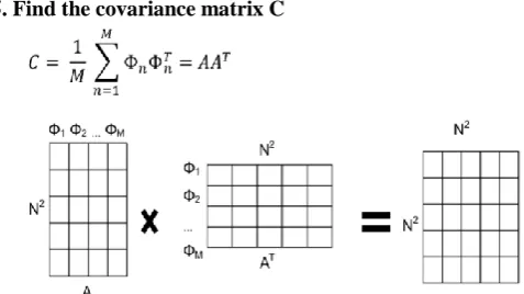
[image:2.595.321.524.507.566.2]

5. Find the covariance matrix C

Figure 3: Computation process with multiplication.

Then, the variance is calculated maintained the Φn. The

vectors Φn are classified to represent the matrix A. The

variance matrix C is processed by increasing the matrix A with the transposition of it and it alluded to as AT.

Equation (3) is the connection between a matrix A, its eigenvectors and its eigenvalues

=

−

₄

=0

(3)

= =

4 =

To get the eigenvalues, the following is the formula

Det( − $ =0) (4)

The matrix A given below is an instance to demonstrate the process to figure the eigenvalues.

(5)

The scalar is multiplied with the identity matrix of size A matrix. Accordingly, two eigenvalues are computed. The quantity of eigenvalues depends on the number of rows of the matrix A.

(6)

The two calculations higher than characterize the calculation of det − $ = zero once the equation superior than is solved, the eigenvalues -1 and four square measure obtained. Then the eigenvectors associated with every eigenvalue is calculated by determination the primary equation = with the eigenvalues antecedently achieved. The subsequent instance illustrates the computation with the eigenvalue -1.

(7)

The eigenvector given eigenvalue is -1, and shown in the equation (8) and the similar process is used for computing the eigen values.

(8)

6. Measure the eigenvectors with corresponding eigenvalues.

Here, two decisions to process eigenvectors. It is possible that one tend to compute the eigenvectors (of AAT or the eigenvectors Vi of ATA. These 2 different ways that have a

comparable eigenvalue, and accordingly the connection between the eigenvectors is i = i. AAT gives a network N2×N2 as a lead to

[image:2.595.51.290.612.746.2]

(3)

it may like the different because of regularly; the amount of pictures inside the training set is littler than the quantity of pixels. In this way, it is quicker to achieve the figuring. ATA have the limit of M eigenvalues and also eigen vectors in spite of AAT which may achieve an assortment of N2

eigenvalues and also eigenvectors. These M eigenvalues speak to the most significant eigenvalues encased to N2.

These eigenvectors (should be standardized, and furthermore the social control must rise to one, ∥ i∥ = 1). The norm of a vector actually symbolizes the length of the vector. The Pythagorean rule is provides for scheming the norm. This rule provides that during a triangle, the sq. of the hypotenuse equivalent to the addition of the squares of the 2 different sides. It implies x2 + y2 = v2. In the example below the norm of the

[image:3.595.388.459.118.161.2]

∥ ∥=

Figure 4: Norm representation. 7. Obtain Eigenvectors

These M eigenvectors are arranged in falling order supported the eigenvalues. Only K eigenvectors are continuous. K is smaller than M and is determined by the algorithmic rule. All the coaching photos are often pictured by a mix of the K eigenvectors.

(9)

= The quantity of eigenvectors Z = The eigenvectors at the index Φi = The Image - the average.

Here, each eigenvector that is additionally recognized as eigenface symbolizes a district of every image within the coaching knowledge. The picture may be rotten through every eigenface. Every projection is the vector that has been computed with the picture and an eigenvector. The square measure projections, wherever represents the number of relevant eigenvectors.

Figure 5: Square measure of k projections.

= the projection of the image " " with the eigenvector index "1".

= the quantity of eigenvectors for kept.

Face recognition with an unfamiliar image:

To start with, the picture is changed over into a vector Γi and

subtract the mean as it has been done as of now while setting up the AI (Φ = Γ − Ψ) Then, the image is foreseen into the eigen space with

(10)

The eigenspace holds all the eigenvectors. Further, Φ is associated through the Eigenfaces so as to actuate the projections.

[image:3.595.92.245.242.301.2]

Figure 6: K x 1. representation

Finally, to search the picture inside the training set that has the slight separation to investigate the picture. The below mentioned formula signifies the association among Ω of the take a look at image and Ωi wherever is that the photos of the coaching set. The category of the nearest image can predict the person of the unfamiliar image.

_{e =} ∥_Ω−Ωi∥ (11)

A geometer remove is wont to understand the shortest face. Nonetheless, it confirmed that the Mahalanobis separate is more often than not extra right is contrasted with an edge and if is littler, it will affirm that the face has a place with an individual United Nations office isn't inside the instructing set, so the picture is added to schooling set as a fresh out of the box new individual. Something else, the picture is utilized as a fresh out of the plastic fresh picture for schooling the perceived individual and is furthermore included into the instructing set with the linked mark. Then the calculation could be a consistent AI and is intended to turn into extra dependable at whatever point a fresh out of the box new check is executed because of the components of the instructing set will increment perpetually.

II. THE FISHERFACES

Fisherfaces conjointly employs a holistic method. This algorithm will be an amendment of Eigenfaces, therefore conjointly employs most important parts of Analysis [4]. The most adjustment is that Fish- faces take into thought categories. Because, it has been aforementioned antecedently, Eigenfaces doesn't create the distinction between two images from completely dissimilar categories throughout the coaching half. Every image was suffering from the entire average [5]. Fisherfaces utilizes the strategy Linear Discriminant examination so as to create the distinction among two photos from a unique category. The point is to diminish the variety among a class contrasted with the variety among categories. For that not just the complete average of countenances is utilized, however the normal per class will likewise be a basic task. The average is determined with the accompanying recipe where , the class and is the quantity of pictures in the class .

(12)

[image:3.595.125.230.581.639.2]

(4)

(13)

Now, the scatter matrixes are computed. The Intra-class scatter matrix symbolized by Sw and can be acquired with the

help of the following equation

(14)

The Inter-class scatter matrix is indicated by Sb which is

computed as follows:

(15)

The next formula will be used to obtain the total scatter matrix

S

T.

(16)

The objective is to determine a projection of

"

which make the most of Fisher’s optimization criteria.

(17)

The eigenvectors are found as follows:

_b ₍

=

₍ _w ₍

,

= 1,2,...

(18) Then at that point the strategy is equivalent to prime component Analysis. The prediction of the training picture is contrasted and the prediction of a check picture, and furthermore the picture class that has humblest separation is the expectation of the algorithmic principle.

III. THE LOCAL BINARY PATTERNS

HISTOGRAMS (LBPH)

[image:4.595.333.519.55.131.2]

This algorithmic rule conjointly needs grayscale photos for process the schooling [6]. The constituent within the center is evaluated to its neighbours. Every neighbour that is smaller than the constituent within the middle, the worth zero are added to the threshold sq. (figure 6) that stores the result or a one is to be added. The threshold sq. and weights sq. is not present within the image, they are only a representation to know the method. When comparisons are completed, every result is increased by a weight and every constituent includes a weight to the ability of 2 from 2x to 2y. Every constituent within the centre of a 3×3 sq. has eight neighbours[7]. These eight pixels represent one computer memory unit that explains the victimization of these weights. The weights area unit affected in an exceedingly round order however, the burden of a constituent doesn't a modification. For instance, if the constituent prime left includes weight of 128, and it will keep the weight for all the assessments within the image[8]. Then, the added weights is considered and becomes the worth of the constituent within the middle of the sq.. The Figure 6 shows the results of the associations and therefore the weight that is expounded to every constituent.

Figure 7: The results of the comparisons

Figure 6 shows the instance sq. characterizes a 3x3 pixels sq.. The brink sq. stores the results of the comparison created within the example sq.. The weights sq. is used to understand the load of every picture element within the example sq[9].. The calculation is the sum of every picture element within the threshold per their weight provides a new value of the pixel within the mid of the instance sq.

This methodology is done for every bit of picture and the image is isolated into a particular quantity of areas. And then, a histogram is expelled since each zone and all of the histograms are connected. For seeing a face, the extremely same methodology pear-formed aped, and the last histogram is appeared differently in relation to each and every histogram in the planning data. The name related to the neighbouring histogram is the desire for the count. When it comes to crowd locator view, this figuring isn't delicate to an assortment of radiance.

The LBPH is altered in various ways and one is named as Extended LBPH. This type of augmentation is utilizing a roundabout neighbourhood which is made of radiuses and various inspecting focuses. This methodology enables a pixel to have in excess of eight neighbours. Contingent upon the sweep (figure 7), the pixel in the centre can be evaluated are de-specification pixels which are not beside it[10]. Another expansion is termed as uniform example.

[image:4.595.307.541.588.671.2]

The augmentation contemplate is the quantity of progress in the outcome byte. One progress is, by an adjustment in the byte from a 0 to a 1 or a 1 to a 0. For instance, 00000001 has one progress and, 00011000 has two advances. It is demonstrated the designs with various changes from 0 to 2 are the most well-known. The examples with two or less changes more often than not have a particular meaning how it very well which is identified in figure 7. All histograms with multiple advances will be regrouped together. The adjustment makes the vector speaking to these histograms littler.

(5)

IV. THE

CONVOLUTIONAL

NEURAL

NETWORK

The convolutional neural is one more approach to achieve face response. The CNN has architect structure that empowers to utilize 2d pictures as data sources. A CNN comprises of a few layers will be called shrouded layers. The layers will make of a few neurons. A neuron has explicit weight and gets information. The contribution of the primary layer is an image of a face. The yield of the last layer is tpredictedted class, which is the individual. So as to have a superior appreciation of trecognitionion process, here it is desirable over utilize a simple precedent. Subsequently, 'X' and 'O' are utilized as classes rather than people. The target of this model is to foresee whether the information is a 'X' or 'O'.

The Convolution layer

Every pixel in the image is in between - 1 and 1. '- 1' is a dull pixel, and 1 is a splendid pixel, '0' is dim. And by (figure 8) which speaks to a 'X' and notice three highlights which are utilized to draw the 'X'. There is one example speaking to a back-ward-slice, another, a forward cut and the last one across. Here, sample examples are utilized as channels and will attempt to be coordinated through those photos.

Figure 9: which speaks to a "X"

Figure 8 shows the portrayal of an image of a 'X' with the qualities comparing to the shade of every pixel. The numbers are from '-1' to '1', where the most modest number is the dimest. The examples to recognize an 'X' are extricated from the picture.

The one of the channels is picked and is contrasted with other hinders the image. A channel compared to a square with a similar amount of cells. Here, the channel is first contrasted with the upper left square of the image with a similar scope. This process is rehashed over the complete picture. Later a correlation of a square, it transfers from the present position to the following square.

[image:5.595.308.542.105.188.2]

For deciding the transfer starting with one square then onto the subsequent, the walk must be taken in consideration. A walk speaks to the quantity of pixels that is moved on from the pre position. For instance, if covering ought to be kept away from when playing out the correlation, the walk must be at any rate that as large as the length of the channel, with 3x3, the walk must be no less than 3 for not having one pixel used in more than one square figure 9. The channel is ‘n’ press in grant a square of 3×3 unique sizes are conceivable. Add a zero to the picture and it includes some additional pixels all over the image with the esteem '0'. The estimation of zero states to the quantity of zero layer about the picture. For an instance, in figure 9 with a walk of 3 the following movement and later the correlation are 2. The

[image:5.595.376.476.245.347.2]

figure 10 demonstrates visualization of a zero. The target of 0 is to check the measure of the yield. By including a buffer, it is conceivable to get a yield with a similar size of information estimate.

[image:5.595.51.288.356.457.2]

Figure. 10: The Perception of a move after an examination Figure 9 shows the perception of a move after an examination with a walk 1 and a walk 3. A walk of a similar size of the channel withholds from covering

.

Figure 11: Perception of a buffer 2 encompassing an image. Every examination will give one number and it implies after every one of the examinations, it have another square a lot littler than previous. The span of the subsequent square relies upon various components:

1. The extent of the picture

2. The measure of the channel

3. The estimation of the walk

4. The span of buffering.

The accompanying equation can be utilized to predict the span of the subsequent square.

(19)

= h h h / h = h h h / h

= h = h = h h

The figure 11 shows the output size formula. For an instance, if information square of 9×9 with a channel 3×3, with no buffering and a walk of 1, it has a yield of 7×7. Expected square declares to X. Here, one will attempt to coordinate to the forward cut channel of the image and is shown in figure 8. For contrasting a channel and another square, every pixel in the channel is increased by the related pixel in the correlation square. The outcome is put away in another cluster. At that point, the total of all numbers is determined lastly, get the normal by isolating the entire with the quantity of pixels in the channel. The normal square is the last outcome for the

(6)

put away in the yield square.

The figure 12 represents the correlation between a channel and the examination square. In an ex-abundant, the correlation square is indistinguishable to the channel. The correlation of two indistinguishable pixels offers the esteem 1, in this way contrasting with an indistinguishable square will have a square brimming with 1 accordingly, and the normally 1. As an update, the pixels can be between - 1 and 1, however to make the precedent more clear, just highly contrasting pixels have been utilized.

The figure 12 shows the perception of an examination among a channel and a square which identical. The duplication among each comparing pixel is processed and the affirm phase of the subsequent square is determined. The normal comes out to the pixel it related in the square yield.

[image:6.595.380.488.52.178.2]

Figure 12: Perception of an examination between a channel and a square.

In figure 13 the regressive cut channel is contrasted with a square which isn't the equivalent. Indeed, the increase among the channel and also the other square is executed. At that point, the total will be determined, and at long last get the normal by separating entirety by 9. The analyzed square is diverse by this time, and shows the outcome is littler with an estimation of 0.33.

Figure 13: Perception between a channels which is distinctive to the thought about square.

[image:6.595.329.544.220.391.2]

[image:6.595.51.290.244.374.2]

Figure 14: Visualization of the o/p square after estimating the filter backward slash

Figure 15: Hallucination of the outputs square after evaluating all the filters.

When the procedure is rehashed for each square, figure 14 is the result. The example in reverse slice is unmistakable in outcome which is a similar example as the channel utilized for the examinations. The outcome is a square 7×7 as anticipated by the recipe. The whole procedure is additionally performed for different channels which are shown in figure 15. The outcome with the procedure is known as the convolution layer and this yield is utilized as contribution to one more layer. There is no standard for picking the hyper parameters, those are the diverse components utilized in tformula figure 11. They rely upon the sort of information, the multifaceted nature of the pictures as well as different components.

CONCLUSION AND FUTURE SCOPE

The experiment demonstrates, all these algorithms are relatively accurate. However, OpenFace is more accurate and reliable in comparison with the others.

Eigenfaces is not exceptionally sensitive to an adjustment in the number of subjects amid the principal stage, an expansion in size of the preparation set helped the calculation to address its wrong expectation. This reflection is the inverse with the tests in another condition. An expansion in the informational collection did not perceive more subjects however it transformed right expectations into improper ones. Eigenface is not precise in the second stage. Fisherfaces do well, to

[image:6.595.49.285.502.632.2]

(7)

may, its conduct was diverse in the second stage. Some of the time with 20 pictures, the outcomes are better; however with 40 pictures the outcomes are equivalent or more terrible. This calculation is more often than not the most exceedingly awful in the two stages. It additionally has low exactness in the second stage. LBPH dependably in any event 96% in the principal stage and is the next-best calculation. In the second stage, this calculation results a drop in the precision which contrast with the primary stage. It is not as much as exact than Eigenfaces. An expansion in the quantity of issues drastically changed its expectation. In each stage, an expansion in the preparation information has a constructive outcome or no impact. OpenFace is the perfect and best calculation method. It perceived splendidly every one of the photos in the main stage and organized with 5 and 10 subjects in the later stage. It has specific errors in the later stage with 15 subjects. These mistakes are limited with bigger preparing information. OpenFace is affected by an adjustment in the earth compared to the others which experienced issues to perceive the photos. In light of these outcomes, one can infer a convolutional neural system which is more proficient for playing out a facial acknowledgment than a measurable methodology or looking for examples. OpenFace can be enhanced by testing distinctive hyper parameters and various mixes of shrouded layers. Expanding the measure of information in the data index for separating the highlights is likewise an approach to conceivably improve the outcomes. Another theme, which is utilizing a similar methodology as facial acknowledgment is recognition. Rather than separating people, the point is to perceive the feeling of an individual. The idea of class is additionally utilized, in spite of the fact that as opposed to having an individual speaking to a class it is an outward appearance, for example, upbeat, pitiful, astounded, dread, outrage or impartial. Fisher-face or a convolutional neural system is utilized for perceiving feelings because of their way to deal with group pictures.

REFERENCES

1. Y.Taigman, M.Yang and M.Ranzato Deepface: Closing the gap to humal- level performance in face verification, CVPR IEEE Conference, 2014.

2. M.Weinberger, Facebook vs. Snapchat in computer vision - Business Insider. 11 May 2017.

3. M. Geitgey, Modern Face Recognition with Deep Learning, Business Insider, 11 May 2017.

4. S.Jaiswal and M. Gwalior, Comparison between face recognition algorithm-eigenfaces, fisherfaces and elastic bunch graph matching,

2011.

5. N. Morizet, F.Rossant, F.Amiel, and A.Amara,

2D du visage pour , 2006.

6. T.Ahonen, A.Hadid and M.Pietik, Face Recognition with Local Binary Patterns, 2004.

7. B.Amos, B.Ludwiczuk, and M.Satyanarayanan, OpenFace: A general-purpose face recognition library with mobile applications,

2016.

8. V. Nair, and G.E. Hinton, Rectified Linear Units Improve Restricted Boltzmann Machines. 2010.

9. M.Turk and A.Pentland, Eigenfaces for Face Detection / Recognition. Journal of Cognitive Neuroscience, 1991.