From Source to Surface: The dynamics of heterogeneous mantle plumes

(1)

From source to surface: the dynamics of heterogeneous mantle plumes

Linking plume-generated volcanism to deep mantle structure and composition

A thesis submitted by

Timothy D. Jones for

the degree of Doctor of Philosophy

of

The Australian Nation University Canberra, Australia

March 2018

c

(2)

Abstract

This thesis is a compilation of three papers investigating the relationship between mantle plume dynamics, Earth’s thermo-chemical structure, and geochemical trends recorded by volcanic hotspots, using numerical simulations that are supported by geophysical and geochemical data sets. The results show that hotspot lavas reveal a wide range of dynamical plumes behaviour previously unrecognised, and that the systematic geochemical trends recorded in hotspot lavas have a complex relationship with deep mantle structure and composition.

Paper 1 demonstrates that physical property variations across deep-mantle structure influence the structure of mantle plumes, geochemical trends recorded by hotspot lavas are unlikely to reflect large-scale chemical domains in the deep-mantle, and stable, long-lived, chemical ‘piles’ in the deep-mantle will be sampled at the centre of plume conduits. The paper reports results from a suite of numerical models in which the compositional structure in the deep-mantle is tracked through an evolving mantle plume, where the density and rheology of compositional structure in the deep-mantle is varied with respect to the ambient deep-mantle. Results indicate that deep-mantle plumes only preserve deep-mantle composition when such variations in density and rheology are negligible.

(3)

(4)

Declaration

This thesis includes 3 original papers that have been previously published/submitted for publication in peer reviewed journals. The proper citation for each paper is given at the beginning of their corresponding chapters. Each paper incorporates material that is result of joint research. I hereby declare that, in all cases, I was the lead researcher and conducted themajorityof the work on the individual elements that follow:

1. Formulation in the concept phase of the basic scientific problem on the basis of theoretical questions which require clarification, including a summary of the general questions which it is assumed will be answered via analyses or concrete experiments/investigations.

2. Planning of data collection/analyses and formulation of investigative method-ology to address those questions developed in (1), including choice of method and independent methodological development.

3. Involvement in carrying out the methods and analyses of results.

4. Presentation, interpretation and discussion of the results obtained in the form of an article or manuscript.

I declare that, to the best of my knowledge, this thesis does not infringe upon anyones copyright nor violate any proprietary rights and that any ideas, techniques, quotations, or any other material from the work of other people included in this the-sis, published or otherwise, are fully acknowledged in accordance with the standard referencing practices.

Timothy Jones Lead author

(5)

Acknowledgements

(6)

List of Figures

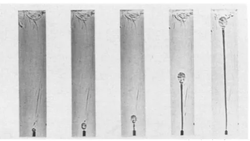
1.1 Fluid model of low viscosity plume rising through a high viscosity environment illustrating its head-tail structure. After Whitehead and Luther (1975). . . 19 1.2 Maps of large igneous provinces (LIPs). Dotted lines show the known or

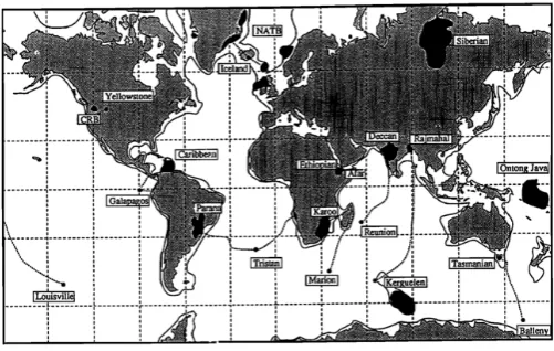
conjec-tured connections to active volcanic hotspot tracks. After Duncan and Richards (1991). . . 20 1.3 Injected lab plume that shows location of source versus entrained material. The

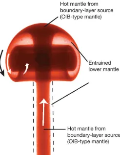
dark-coloured fluid is from the hot boundary-layer source of the plume, whereas the light material is cooler overlying fluid that was entrained into the rising plume. In the case of the mantle the dark-coloured material is from the thermal boundary layer above the core, whereas the light material is entrained lower mantle. The entrained light material makes up the largest portion of the head, with minor amounts on the edges of the conduit. The conduit is predominantly the dark material ascending from the source region. After Campbell and Griffiths (1990). . 21 1.4 a) Numerical model of evolving plume originating from a thermal boundary layer

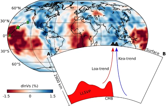
showing temperature field. b) Zoomed in view of plume from a) in final panel showing distribution of tracers coloured by their initial position. Tracer distri-bution shows that material primarily sourced from bottom 150 km and that any entrainment from shallower depths is negligible. After Farnetani et al. (2002). . . 22 2.1 The Hawaiian hotspot (green star), plotted above the shear-wave tomography

(9)

2.2 Regime diagrams for conduit structure as a function of the Buoyancy Number,

B, and theδparameter controlling the temperature dependence of viscosity. Dia-grams are presented for 3 different scenarios, where the viscosity contrast between the chemical reservoir and surrounding mantle, ˆηc, is: (a) 0.1; (b) 1; and; (c) 10.

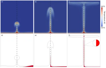
Bilaterally asymmetric and concentric regimes are denoted by blue crosses and red circles, respectively.. . . 35 2.3 (a)-(c) snapshots of the temperature field from a case where B = ∆ρc = 0.0,

ˆ

ηc = 1, andδ = 2. The solid black line is theT = 1660 K temperature contour,

whilst the dashed black line highlights the plume’s central axis; (d)-(f) simulta-neous snapshots of the compositional field (red), where φ= 0.5, showing how a bilaterally asymmetric structure is preserved in the conduit as material ascends to the surface. Note that the inset shown in (f) represents a schematic cross-section of the inner conduit. . . 37 2.4 As in Fig. 2.3, but for a case that adopts a concentric plume structure, where B =

0.5, ∆ρc= 0.75%, ˆηc = 1, andδ= 2. Under this scenario, the spatial distribution

of geochemical domains in the lowermost mantle is not preserved during plume ascent. . . 38 2.5 (a)-(c) temporal snapshots of a 3-D simulation for a case whereB = ∆ρc = 0.0,

ˆ

ηc = 1 andδ= 2. The blue isosurface atT = 1823 K outlines the plume, whilst

the red isosurface delineates the reservoir interface at φ= 0.5, which illustrates how bilateral asymmetry develops within the conduit as the simulation evolves. . 39 2.6 Snapshots of the two dominant conduit regimes identified in this study. In both

cases we plot a blue isosurface atT = 1823 K and the reservoir interface (red) at

φ= 0.5. The model parameters are: (a) bilaterally asymmetric: B= ∆ρc= 0.0,

ˆ

ηc= 1, andδ= 2; and (b) concentric: B = 0.5, ∆ρc = 0.75%, ˆηc= 1, andδ= 2.

(10)

2.7 Plot of effective (local) buoyancy number across the base of the plume conduit illustrated in Fig. 2.4. Black lines are temperature contours at T = 1750, 1820, 1890, 1960 and 2040 K. The increased temperature at the conduit centre results in a corresponding decease in effective buoyancy number, illustrating why a plume can more readily sample dense material at its centre relative to its periphery. Note that this plot assumes that dense material, with ∆ρc = 0.75%, is present

everywhere. . . 41 3.1 a) (1)-(5) temporal snapshots of the temperature field from a case whereB = 0.5

andhc= 75 km; (6)-(10) simultaneous snapshots of the compositional field (red),

where the solid black line is the T = 1623 K contour. Snapshots are mirrored along the domain’s left-hand boundary. Under this scenario, both the plume head and tail transport dense material towards the surface; b) as in Fig. 3.1a, but for a case where B = 0.6. Under this scenario, the increased thermal buoyancy of the plume head is able to advect dense material. However, this dense material is unable to rise through the comparatively low buoyancy plume tail; c) as in Fig. 3.1a, but for a case whereB = 1.0. Under this scenario, the dense layer remains at the base of the model, with the plume derived solely from overlying ambient mantle material. . . 52 3.2 Maximum values ofRc as a function of Buoyancy number for: (a) plume heads;

and (b) plumes tails. Rc for plume tails is defined 30 Myr after the maximum

value of Rc in plume head is reached. Both panels illustrate that the increase

in B results in a reduction of Rc, as less dense material is entrained. At each

value ofB, voluminous plume heads consistently yield higherRc than their tails

due to their larger thermal buoyancy; c) plot of Rc (black) and the buoyancy

flux (dashed grey) from the case illustrated in Fig. 3.1b. The initial spike in buoyancy flux reflects the plume head passing through the upper mantle. The head has sufficient thermal buoyancy to advect dense material, causing the spike inRc. The flattening of both curves reflects the rise of the plume tail through the

(11)

3.3 a) Temporal evolution of Rc for three cases, where B = 0.3 (red), 0.6 (green)

and 1.0 (blue). Note that time zero begins whenRc exceeds 0.1%. In all cases

the dense layer has an initial thickness of 75 km; b) temporal evolution ofRc for

three cases, whereB = 0.6 andhc = 25 km (red), 75 km (green) and 200 km (blue). 55 3.4 Snapshots of both the compositional and temperature fields for a case where

dense material ponds around the upper-lower mantle boundary. Parameters are the same as in Fig. 3.1b except that the dense layer is initially 200 km thick. The excess density of material at the base of the model prolongs plume initiation, allowing the TBL to thicken and spawn a wider plume, which contains more dense material. Reaching the upper mantle, the plume loses enough heat such that the dense material is no longer buoyant and, subsequently, ponds. Ambient mantle material, on the other hand, rises through the upper mantle and reaches the base of lithosphere. . . 55 3.5 (a) snapshots of temperature and compositional fields, with both dense material

(red) and ultra-dense material (black), where parameters are the same as in Fig. 3.1b except the dense layer is 65 km thick and model is initiated with ultra-dense material along its base, which is 10% denser than background mantle and 10 km thick; (b) zoomed in snapshots of bottom right corner of (a) 8 - 10, illustrating the evolution of ultra-dense material as it moves along the edge of the overlying dense accumulation and into the plume conduit. . . 57 3.6 Plot of data from Fig. 3.5: red and blue lines denote theRc diagnostic for dense

and ultra-dense material, respectively. In contrast to Fig. 3.3, the y-axis has a log-scale to reflect the orders of magnitude difference inRcfor both components.

The initial pulse in dense layer material tracks the head as it passes into the upper mantle, with the subsequent flattening tracking the tail. Roughly 25 Myr after the pulse in dense layer material, there is an increase in the proportion of ultra-dense material within the plume’s tail, which gradually increases with time. 58 3.7 Model results showing contribution from positive W reservoir (black) and core

(red) in generating µ182W when mixed with an upper mantle reservoir with a

µ182_{W value of 0. The grey shaded region shows the spread of values observed}

(12)

3.8 Regime diagram for conduit structure as a function of the buoyancy number,B, and the initial thickness of the compositional layer. We define three regimes to describe the compositional structure of plumes: (i) plume head and tail sample both ambient mantle and dense layer material (blue shading with crosses), where dense material makes up at least 1% of total plume material throughout the simulation; (ii) plume head and tail predominately sample the ambient mantle (green shading with green triangles); and (iii) dense material makes up at least 10% of the plume head and, at most, 1% of the plume tail (red shading with red dots). The blue striped region reflects simulations where dense material entered the upper mantle but stalls below 300 km depth, without reaching the base of the lithosphere. Markers indicate the parameters for which a simulation was run, and shading indicates the extrapolated regime that surrounding parameters are assumed to fall within. . . 60 4.1 Bathymetric map of recent Hawaiian volcanism, highlighting the Loa and Kea

tracks: solid lines represent the geochemically distinct Loa (blue) and Kea (red) volcanic trends Abouchami et al. (2005); Weis et al. (2011). The dashed lines are an estimate of the future projection of these trends based upon our hypothesis. Prior to the emergence of the Loa and Kea tracks, Kea-type lavas are overlain by Loa-type lavas at Ko’olau and Kaua’i Garcia et al. (2010); Weis et al. (2011). The encircled number indicates the approximate age at which Loa trend lavas first appeared at Ko’olau.. . . 70 4.2 Schematic diagram of the tilted Hawaiian plume, the overlying Pacific plate and

(13)

(14)

(15)

4.5 Simulation of a 3D mantle plume beneath a moving plate: the plume is contoured at a temperature of 1673 K. The model domain is outlined by thick black lines. plate-motion is indicated by white arrows. Melting of eclogite, peridotite and pyroxenite is contoured at half the maximum melt rate, thus highlighting the regions of maximum melt productivity for each component (see Supplementary Material to Paper 3, section 7.2.4). For eclogite, melting initiates at a depth of

(16)

4.6 Instantaneous versus gradual changes in the direction of plate-motion: a, Results from the model presented in Fig. 4.5, where an instantaneous change in plate-motion direction of 20◦ was imposed. The plotted lines are: (i) the azimuth of the imposed plate-motion (blue dashed line), and; (ii) the azimuth of a straight line between the melt-rate maxima for peridotite and pyroxenite (black dots with green dotted line). Initially, the two azimuths are parallel (not shown), but after the change in plate-motion direction they are offset by 20◦ and slowly converge over time, with realignment by 8 Myr. b, Results from a model where a gradual change in plate-motion is imposed (otherwise identical to the model in (a)), and data on the azimuthal change in Pacific plate-motion at Hawaii from our kine-matic reconstruction presented in Fig. 4.3 (red solid line). In contrast to the instantaneous case (a), the two azimuthsgradually diverge following the change in plate-motion direction at 6 Ma. The offset between the two azimuths reaches a maximum at ∼2 Ma, when the change in plate-motion direction ceases, and the offset decreases (but remains significant) towards the present-day. . . 79 7.1 Bathymetric maps of Pacific plate hotspots with recent double volcanic tracks:

(17)

(18)

List of Tables

2.1 Parameters common to all cases examined and their reference values. . . 33 2.2 Distinct material properties of all cases examined. B = Buoyancy number; ∆ρc

= chemical density contrast between the reservoir and background mantle; δ= parameter controlling the temperature dependence of viscosity; ˆηc = viscosity

contrast between the reservoir and background mantle. . . 34 3.1 Parameters common to all cases examined and their reference values. . . 51

(19)

Introduction

Plate tectonics is the unifying theory of Earth sciences, but it is somewhat in-complete. Describing only the motions of the plates but not the forces that move them, plate tectonics is a kinematic theory. A more fundamental theory, implicit to plate tectonics, is mantle convection: a dynamical theory of geology that describes the underlying forces that move and shape Earth’s crust, as well as its rocky inte-rior. Convection, more generally, appears to be a ubiquitous process throughout the planet, dictating the transfer of heat in the atmosphere, oceans, and outer core, and is essentially what makes Earth a dynamic system. It involves two basic physical processes: buoyancy-driven fluid flow and thermal conduction.

Thermal conduction essentially sets the scene for fluid flow by establishing horizontal density gradients that become unstable through their own buoyancy and either rise or fall through the interior of the fluid. In the mantle, the main horizontal density gradients occur at thermal boundary layers (TBL), one at the surface and one at the core-mantle boundary (CMB). The bottom TBL is caused by an influx of heat from the core, and the top TBL is caused by an outflux of heat through the the litho-sphere, which subsequently loses heat to the oceans, atmosphere and, ultimately, space. These two TBLs operate quite differently, establishing two distinct modes of convection. Cooling oceanic lithosphere eventually becomes negatively buoyancy and sinks into the mantle in the form of subducting sheets. Hot material sitting on the CMB becomes positively buoyant, upwelling through the mantle as columns of rock, known as mantle plumes. Although mantle convection is dominated by the surface TBL and the process of subduction, a growing body of evidence suggests that the bottom TBL plays a central role in governing its behaviour, through shap-ing deep mantle structure and generatshap-ing the mantle plumes that drive it to the surface.

(20)

[image:20.595.200.453.54.196.2]

Figure 1.1: Fluid model of low viscosity plume rising through a high viscosity environment illustrating its head-tail structure. After Whitehead and Luther (1975).

plates, formation of mineral deposits, as well as features of the deep Earth, such as the geodynamo, Earth’s internal heat budget, the behaviour of mineral-phase trans-formations, seismically inferred features of the mantle and inversions of the geoid. More recently, mantle plumes have been invoked to explain phenomena beyond the sold-earth: from long-term variations in sea-level, to climate change, mass extinc-tions, and even the development of the Martian mantle. Despite an increase in the breadth and depth of observations, research into the richness of dynamical plume behaviour, which such observations imply, has lagged. The research presented here helps to close this gap.

The history of mantle plumes is often traced back to Wilson (1963), pre-dating the concept itself. Wilson first recognised that there are around 40 volcanic island chains across the planet that are not associated with tectonic plate boundaries and seem to remain fixed relative to one another as the overlying plates moved around. He hypothesised that the source of such volcanism was a ‘mantle hotspot’, which remained in regions of low convective velocity, such as the centre of convective cells. This built on some of the earliest inferences about the volcanic island chains on the Pacific plate, which seemed to age progressively along the chain. It was Morgan (1971, 1972) who later proposed that the source of the eruptions were, instead, mantle plumes: columns of hot, buoyant rock that originate at the core-mantle boundary.

(21)

[image:21.595.201.452.56.215.2]

Figure 1.2: Maps of large igneous provinces (LIPs). Dotted lines show the known or conjectured connections to active volcanic hotspot tracks. After Duncan and Richards (1991).

is used herein to describe the volcanic surface expression of plumes and not the original concept employed by Wilson. Much of what was proposed in Morgan’s original paper (Morgan, 1971) was validated in the decades that followed. For example, the correspondence of estimates of heat transported by plumes and the estimates of heat flow from the core (Stacey and Loper, 1984), vindicated Morgan’s proposal that plumes originated from a thermal boundary layer at the base of the mantle. From this perspective, it was understood that plume’s were the convective manifestation of a cooling core. To be sure, aspects of Morgan’s idea have been reworked and updated. For instance, he conjectured that a relatively viscous lower mantle would keep plumes fixed, a good approximation at the time that helped refine plate motions. It is now generally accepted that plumes are frequently deflected by convective flow (e.g. Zhao, 2001), and are not fixed, but move at a fraction of surface plate velocities (Davies and Davies, 2009). Although it was observational evidence from volcanic island chains that established the existence of plumes, our understanding of their dynamic behaviour was propelled by mathematical results and elegant laboratory experiments on fluids that are analogous to the mantle, despite operating on observable time-scales.

(22)

[image:22.595.264.387.56.214.2]

Figure 1.3: Injected lab plume that shows location of source versus entrained material. The dark-coloured fluid is from the hot boundary-layer source of the plume, whereas the light material is cooler overlying fluid that was entrained into the rising plume. In the case of the mantle the dark-coloured material is from the thermal boundary layer above the core, whereas the light material is entrained lower mantle. The entrained light material makes up the largest portion of the head, with minor amounts on the edges of the conduit. The conduit is predominantly the dark material ascending from the source region. After Campbell and Griffiths (1990).

resistance from the surrounding mantle. In order to overcome this force, the head of the plume must be sufficiently voluminous and therefore buoyant enough to force a path. Hot material rising up through the conduit provides the head with additional fluid. Hot material rising up through the conduit is displaced at the top of the head, spreading out radially and around its peripheries. As this occurs, heat from the conduit-fed material (source material) is diffused radially, increasing the tem-perature of the surrounding mantle (and plume head), thereby decreasing its density and sweeping it into the head in a recirculating motion. Early laboratory experi-ments showed that the plume head will experience further growth through thermal entrainment of the surrounding mantle throughout their ascent. Small amounts of surrounding mantle were also shown to be entrained along the outer conduit walls of the plume tail. Numerical experiments by Davies (1999), scaled approximately to the mantle, indicate that material entrained in the plume head will come from the lowest 10-20% of the mantle (Fig. 1.3). The extent of such thermal entrainment has since been debated (Farnetani and Richards, 1995; Farnetani et al., 2002; Lohmann et al., 2009), with numerical studies showing that plumes originating from a ther-mal boundary layer experience very little entrainment of the surrounding mantle, and are instead primarily sourced from the thermal boundary layer via advection (Fig. 1.4). This has several important implications for the compositional diversity observed in hotspot volcanism, which will be expanded upon in this thesis.

(23)

perspec-Figure 1.4: a) Numerical model of evolving plume originating from a thermal boundary layer showing temperature field. b) Zoomed in view of plume from a) in final panel showing distribution of tracers coloured by their initial position. Tracer distribution shows that material primarily sourced from bottom 150 km and that any entrainment from shallower depths is negligible. After Farnetani et al. (2002).

tives on Earth’s broad-scale structure is the distinction drawn between the upper and lower mantle. Geochemists had long known that hotspot tracks, or ocean islands basalts (OIBs), and mid-ocean ridge basalts (MORBs), displayed different isotopic characteristics. Once it was recognised that the deep mantle is driven to the surface in plumes and sampled by OIBs, the inference was made that the lower mantle must have a different composition to the upper mantle, which is sampled by MORBs (e.g. White, 1985; Hart and Zindler, 1986). This sparked a long debate about whether or not the mantle was compositionally stratified, where the upper and lower mantle are connectively isolated form one another. I won’t go into the details of the de-bate here, only to say that while some degree of vertical stratification in the mantle is implied by the observed differences in MORB vs OIB chemistry, the hypothesis that there is a hard boundary between the upper and lower mantle, meaning that little mass transferred has occurred, has largely been falsified. This is most evident in images from seismic tomography that show subducted slabs descending into the lower mantle (Fukao et al., 1992; Grand et al., 1997; van der Hilst et al., 1997). Assuming that similar rates of subduction have occurred over geological history, this reflects a large mass flux on its own, which must be doubled to account for the equally large return flow. The result is devastating for any hypothesis requiring a chemically isolated lower mantle (Davies, 1998).

(24)

and a new model of the mantle began to predominate: discontinuous and distributed reservoirs (Tackley, 2000). A model that has received considerable support invokes long-lived ‘piles’ of chemically distinct material in the lowermost mantle (Tackley, 1998; McNamara and Zhong, 2005; Deschamps and Tackley, 2008, 2009). Such ‘piles’, stabilised through excess chemical density, would remain isolated from mantle circulation, for billions of years (Tackley, 2000). Plumes entraining small volume fractions of dense material could subsequently account for geochemical variation between MORBs and OIBs. This presented a new problem: how could discontinuous and distributed reservoirs be mapped, and their properties be inferred, from surface observations?

As plumes drive hot material to the surface, they carry a message from Earth’s lowermost mantle, but, as I will argue throughout this thesis, deciphering this mes-sage is a challenge. Many have assumed that the geochemical trends recorded at by volcanic hotspots at Earth’s surface reflect the large-scale thermo-chemical struc-ture of the deep mantle (e.g. Dupr´e and All´egre, 1983; Castillo, 1988; Farnetani and Hofmann, 2010; Weis et al., 2011; Huang et al., 2011; Farnetani et al., 2012). However, such inferences are problematic, as they ignore a fundamental feature of thermo-chemical convection; not only does the physical process of mantle convection affect the chemistry of the mantle, but chemical changes may also react upon mantle convection, most directly through density, buoyancy, and rheology. In order to ex-ploit the information provided by plumes at the surface in our efforts to deduce the nature of the deep mantle, we must understand how the mantle’s thermo-chemical structure influences plumes, and vice-versa.

This thesis is a compilation of three papers exploring the causal relationship be-tween mantle plume dynamics, compositional structure in the deep mantle, and geochemical trends recorded by volcanic hotspots, through the following research questions:

1. Do mantle plumes preserve the heterogeneous structure of their deep-mantle source?

2. How does the composition of LIPs and OIBs constrain plume structure and the nature of their deep mantle source?

(25)

Pacific plate?

Through each paper, summarised below, I will show that these questions have pro-found implications for plume dynamics. They generate numerous testable predic-tions about plume-related volcanism and the nature of the deep mantle, particularly the seismically inferred large low shear-wave velocity provinces (LLSVPs) and ultra low velocity zones (ULVZs). The approach employed is primarily a forward mod-elling one, in that plume dynamics are simulated using numerical models that have been developed in response to interpretations that link hotspot lavas to features of the underlying mantle. All simulations are conducted using Fluidity, a finite-element based computational modelling framework (e.g. Davies et al., 2011; Kramer et al., 2012).

Do mantle plumes preserve the heterogeneous

struc-ture of their deep-mantle source?

(26)

We demonstrate that this assumption does not hold for compositional domains that differ in their density and viscosity to surrounding mantle, as has been hypothesised for the two Large Low Shear-wave Velocity Provinces (LLSVPs) beneath Africa and the Pacific (e.g. McNamara and Zhong, 2005; Garnero and McNamara, 2008; Bower et al., 2013). When a contrast in physical properties between chemically distinct material and ambient mantle was negligible, the distributed heterogeneity within the plume mapped directly onto the original distribution in the lowermost man-tle. Under this scenario, the chemical variability at sites of plume-related volcanism are a reflection of structure in the deep mantle. However, even small contrasts be-tween the physical properties of chemically distinct material and the ambient mantle changed the result: heterogeneity took an active role in the convective organisation of the lowermost mantle, concentrating dense components toward the center of the conduit and destroying the original material distribution. Such plumes have a con-centric conduit structure. We show the conditions under which each scenario occurs, finding the the latter dominated the examined parameter space, indicating that con-centric plumes are the norm in a chemically heterogeneous mantle, rather than the exception.

This manuscript has been published in Earth and Planetary Science Letters, with the citation: Jones, T.D., Davies, D.R., Campbell, I.H., Wilson, C.R. and Kramer, S.C., 2016. Do mantle plumes preserve the heterogeneous structure of their deep-mantle source?. Earth and Planetary Science Letters, 434, pp.10-17.

Tungsten isotopes in mantle plumes:

heads it’s

positive, tails it’s negative

Paper 2 explores the relationship between the tungsten (W) isotopic compositions of LIPs and OIBs and the deep mantle source from which they originate. We report numerical modelling results that show how the observed tungsten isotope signature of LIPs and OIBs constrains plume structure and has important implications for the structure and evolution of the lowermost mantle. Relative to the modern upper mantle, LIPs have anomalously positive W compositions (expressed via µ182_{W =} [(182_W/184_W

sample / (182W/184W)standard - 1]×106) and OIBs are anomalously

(27)

60 Myr of the solar systems history. Their discovery in recent eruptions is particu-larly surprising as it requires both reservoirs to have survived 4.5 Gyr of convective stirring and mixing. Since many LIPs and OIBs are linked to mantle plumes, with LIPs derived from melting of the plume head and OIBs derived form melting of the plume tail, the positive reservoir must predominate in plume heads, while the negative reservoir must predominate in plume tails.

The results are divided into two related sections. First, using techniques from isotope geochemistry, we quantitatively constrain the relative contributions of positive and negative W sources to LIPs and OIBs, respectively. Second, we run a suite of numerical models of thermo-chemical plumes and search a wide parameter space for reservoir properties that satisfy the calculated relative source contributions to LIPs and OIBs. Taken together, our results indicate that the tungsten isotopic compositions of LIPs and OIBs can only be satisfied for a small portion of the parameter space examined, providing several constraints on the structure of the deep mantle, including reservoir density, thickness, and plume flux. This paper concludes with a discussion of the implications of these results for two consistent features of the lowermost mantle, imaged in seismic tomography models: large low shear-wave velocity provinces (LLSVPs) and ultra low velocity zones (ULVZs).

This manuscript is currently under review at Earth and Planetary Science Letters.

The concurrent emergence and causes of double

volcanic hotspot tracks on the Pacific plate

(28)

noise-mitigated reconstructions of Pacific plate motion over the past 20 Myr, highlighting a recent change in the plate’s azimuthal motion that coincides with the emergence of the Loa and Kea tracks at Hawaii, and 4 other double-volcanic tracks across the Pacific plate (Foundation, Galapagos, Marquesas, Samoa, and Society). The plate motion change is then incorporated into the numerical simulation of the tilted plume. The dynamic behaviour in the model shows that such a change in plate motion will cause the high- and low-pressure melt regions to be exposed as two separate volcanic tracks at the surface, accounting for their concurrent emergence across the Pacific plate. The final part of this study provides an argument, supported by evidence from a series of high-pressure petrological experiments (Yaxley and Green, 1998; Herzberg, 2011), that secondary pyroxenites dominate the low-pressure melt region in eclogite bearing plumes. This final process yields the systematic geochemical differences observed between Loa- and Kea-track volcanism at Hawaii.

The modelling results from this numerical study indicate that double track volcanism is transitory, occurring only when the direction of plume tilt and the azimuthal mo-tion of the overlying plate diverge above a critical threshold. The models show that, eventually, the plume will re-adjust to upper mantle flow induced by the plate, and the double tracks will disappear, re-emerging only with another significant change in plate motion. The corollary to this conclusion is that the appearance of double track volcanism in the geological record may be used as an additional criterion when searching for past changes in plate motion. The papers final conclusions offer sev-eral testable hypothesis implicit in our theory, and a suggestion for future sampling efforts along the Hawaiian-Emperor chain.

(29)

Do Mantle Plumes Preserve the

Heterogeneous Structure of their

Deep-Mantle Source?

T. D. Jones1_{, D. R. Davies}1_{, I. H. Campbell}1_{, C. R. Wilson}2 _{and S. C. Kramer}3 1_{Research School of Earth Sciences, The Australian National University, Canberra, Australia.}

2_{Lamont-Doherty Earth Observatory, Columbia University, New York, USA.} 3_{Department of Earth Science and Engineering, Imperial College, London, UK.}

(30)

Abstract

It has been proposed that the spatial variations recorded in the geochemistry of hotspot lavas, such as the bilateral asymmetry recorded at Hawaii, can be directly mapped as the heterogeneous structure and composition of their deep-mantle source. This would imply that source-region heterogeneities are transported into, and pre-served within, a plume conduit, as the plume rises from the deep-mantle to Earth’s surface. Previous laboratory and numerical studies, which neglect density and rhe-ological variations between different chemical components, support this view. How-ever, in this paper, we demonstrate that this interpretation cannot be extended to distinct chemical domains that differ from surrounding mantle in their density and viscosity. By numerically simulating thermo-chemical mantle plumes across a broad parameter space, in 2-D and 3-D, we identify two conduit structures: (i) bilaterally asymmetric conduits, which occur exclusively for cases where the chemical effect on buoyancy is negligible, in which the spatial distribution of deep-mantle hetero-geneities is preserved during plume ascent; and (ii) concentric conduits, which occur for all other cases, with dense material preferentially sampled within the conduit’s centre. In the latter regime, the spatial distribution of geochemical domains in the lowermost mantle is not preserved during plume ascent. Our results imply that the heterogeneous structure and composition of Earth’s lowermost mantle can only be mapped from geochemical observations at Earth’s surface if chemical heterogeneity is a passive component of lowermost mantle dynamics (i.e. its effect on density is outweighed by, or is secondary to, the effect of temperature). The implications of our results for: (i) why oceanic crust should be the prevalent component of ocean island basalts; and (ii) how we interpret the geochemical evolution of Earth’s deep-mantle are also discussed.

Introduction

(31)

and Campbell, 1991; Davies, 1992; Farnetani and Richards, 1994, 1995; Leitch and Davies, 2001; Davies and Davies, 2009; Davies et al., 2015b,c). Although mantle plumes represent the only source of volcanism on Earth that directly samples the lowermost mantle, it remains unclear how their variable geochemical expression at Earth’s surface (i.e. the geochemical variations recorded in volcanic hotspot lavas) relates to the heterogeneous structure of their deep-mantle source (e.g. Dupré and Allégre, 1983; Allègre et al., 1996; Tackley, 1998; Hofmann, 2003). For example, the most recent 2-3 Myr of volcanism along the Hawaiian-Emperor chain is defined by two parallel volcanic island tracks, the Loa- and Kea-tracks (Jackson et al., 1975), which exhibit distinct geochemical signatures (e.g. Tatsumoto, 1978; Abouchami et al., 2005). Southern Loa-track volcanoes are generally less depleted, displaying systematically higher208_Pb/204_{Pb at a given}206_Pb/204_{Pb, as well as higher}87_Sr/86_Sr and lower 143Nd/144Nd, when compared to the Northern Kea-track volcanoes (e.g. Abouchami et al., 2005). While several hypotheses have been proposed to explain such systematic variations (e.g. Bianco et al., 2008, 2011; Ballmer et al., 2011, 2013, 2015), the most prominent attributes them to internal zonation within the under-lying mantle plume conduit, which may relate directly to large-scale geochemical domains in the lowermost mantle (e.g. Abouchami et al., 2005; Weis et al., 2011; Huang et al., 2011; Farnetani et al., 2012; Hofmann and Farnetani, 2013; Payne et al., 2013; Harpp et al., 2014).

(32)

[image:32.595.151.505.61.286.2]

Figure 2.1: The Hawaiian hotspot (green star), plotted above the shear-wave tomography model S40RTS (Ritsema et al., 2011) at 2800 km depth, illustrating that Hawaii overlies the boundary between a large region of low shear-wave velocities – the Pacific LLSVP – and surrounding mantle. Under the assumption that the Pacific LLSVP represents a chemically distinct body, Weis et al. (2011) hypothesise that geochemical differences between the Kea and Loa trends reflect preferential sampling of these two distinct sources of deep mantle material.

2009; Schuberth et al., 2009a, 2012; Davies et al., 2012, 2015a), and it is unclear whether or not mantle plumes can preserve the heterogeneous structure of their boundary-layer source region during plume ascent, the interpretation of Weis et al. (2011) and Farnetani et al. (2012) has been extended to several other volcanic island chains in the Pacific, namely Marqueses, Samoa, Society, Galpagos and Easter (e.g. Huang et al., 2011; Payne et al., 2013; Harpp et al., 2014; Jackson et al., 2014). However, observations from the Samoan hotspot appear inconsistent with this hy-pothesis. Samoa lies on the southern margin of the Pacific LLSVP and, accordingly, the northern side of the Samoan plume would be expected to preferentially sam-ple isotopically enriched material: the opposite trend is observed, with the Malu (southern) track exhibiting more enriched compositions, when compared to the Vai (northern) track (Huang et al., 2011).

(33)

it has been recognised, in both numerical simulations and laboratory experiments, that the incorporation of active compositional heterogeneity (i.e. heterogeneity that differs from ambient mantle in its material properties) strongly influences the dy-namics of upwelling mantle plumes (e.g. Tackley, 1998; Jellinek and Manga, 2002; Farnetani and Samuel, 2005; Lin and van Keken, 2006a,b; Davies et al., 2012; Stein-berger and Torsvik, 2012).

In this study we use the computational modelling framework Fluidity (e.g. Davies et al., 2011; Kramer et al., 2012; Le Voci et al., 2014; Garel et al., 2014) to explore the parameter space over which the spatial distribution of geochemical domains in the lowermost mantle is preserved in plume conduits during plume ascent, in 2-D and 3-D. Specifically, we build on and complement earlier studies by, for example, Kerr and M´eriaux (2004), Farnetani and Hofmann (2010) and Farnetani et al. (2012), and examine the effects of density and rheological variations between initially distinct and separate source components on plume stability, source entrainment and the stirring of these components. Included in our parameter search is the density and viscosity range predicted for LLSVPs as possible long-lived, thermo-chemical piles (e.g Tackley, 1998; McNamara and Zhong, 2005; Deschamps and Tackley, 2008, 2009; Cobden et al., 2009). Our goal is to further test the hypothesis of Weis et al. (2011) and Farnetani et al. (2012) in the presence of chemical density and viscosity contrasts between different chemical domains.

Methods

(34)

par-Symbol Parameter Value Units

α Thermal expansion coefficient 3×10−5 K−1

η0 Reference viscosity 5×1020 Pa s

ˆ

ηc Ratio of compositional to reference viscosity 0.1 - 10

-ˆ

ηlith Lithosphere viscosity multiplication factor 100

-ˆ

η660 660-km viscosity multiplication factor 30

-ρ0 Reference density 3300 kg m−3

∆ρc Contrast between compositional and reference density 0.0 - 100 kg m−3

Cp Specific heat capacity (at constant pressure) 1000 J kg−1 K−1

D Mantle depth 2900×103 _m

g Gravitational acceleration 9.8 m s−2

κ Thermal diffusivity 10−6 _m2 _s−1

TSurf Surface temperature 273 K

Tp Background potential temperature 1573 K

TCM B CMB temperature 2073 K

Table 2.1: Parameters common to all cases examined and their reference values.

allel linear system solvers available in PETSc (Balay et al., 1997), that can handle sharp, orders of magnitude variations in viscosity; and (vi) has a novel interface-preservation scheme, which conserves material volume fractions, and allows for the incorporation of distinct chemical components (Wilson, 2009; Garel et al., 2014). In this study, Fluidity’s adaptive mesh capabilities are utilised to provide a local resolution of 1 km in regions of dynamic significance (i.e. at the interface between materials and in regions of strong temperature, velocity and viscosity contrasts), with a coarser resolution of up to 100 km elsewhere.

Key model parameters are provided in Table 2.1. Simulations are undertaken in 2-D square and 3-D cubic domains of dimension 2900 km. Boundary conditions for temperature areT = 273 K at the surface,T = 2073 K at the base, with insulating (homogeneous Neumann) sidewalls. Velocity boundary conditions are free-slip and no normal flow at all boundaries. The material volume fraction, φ, is 1 inside the chemically distinct reservoir and 0 elsewhere. A 100-km thick stiff lithosphere is imposed at the top of the model, with a linear temperature profile between surface and underlying mantle. A temperature dependent viscosity is utilised, following the relation:

η(T∗) =η0exp−bT ∗

(2.1)

whereT∗ = (T−TSurf)/(TCM B−TSurf) is the non-dimensionalised mantle

(35)

B ∆ρc (%) δ ηˆc

[image:35.595.241.410.54.190.2]

0.0 0.0 0,1,2 0.1, 1, 10 0.025 0.0375 0,1,2 0.1, 1, 10 0.05 0.075 0,1,2 0.1, 1, 10 0.1 0.15 0,1,2 0.1, 1, 10 0.25 0.375 0,1,2 0.1, 1, 10 0.5 0.75 0,1,2 0.1, 1, 10 0.75 1.125 0,1,2 0.1, 1, 10 1.0 1.5 0,1,2 0.1, 1, 10 2.0 3.0 0,1,2 0.1, 1, 10

Table 2.2: Distinct material properties of all cases examined. B = Buoyancy number; ∆ρc =

chemical density contrast between the reservoir and background mantle; δ = parameter control-ling the temperature dependence of viscosity; ˆηc = viscosity contrast between the reservoir and

background mantle.

by ˆηc. The temperature dependence of viscosity is controlled byb = ln(10δ), whereδ

varies from 0 (isoviscous) to 2 (the maximum temperature induced viscosity contrast examined herein).

In our 2-D simulations a mantle plume is initiated in the lower thermal boundary layer (TBL) at the domain’s centre via a Gaussian-shaped temperature perturbation, which is 200 km in height and 180 km between inflection points. The temperature is equal to Tp at the peak of the perturbation and increases linearly to TCM B at

the base of the model. A distinct geochemical reservoir (φ = 1) is initialised in the domain’s lower right hand corner with a Gaussian-shaped upper boundary. The reservoir material peaks at the domain’s right hand boundary, at a height of 200 km, and has an inflection point 290 km left of the peak. In our 3-D simulations the plume is initialised at the centre of the domain within the lower TBL. We use a Gaussian-shaped temperature perturbation with the same dimensions as in the 2-D case, except that the distance between inflection points applies radially. The geochemical reservoir is initialised with the same planar dimensions as our 2-D case but is extended throughout the domain’s entire 3-D extent.

We vary both the density contrast, ∆ρc, and the viscosity contrast, ˆηc, between

the reservoir and background mantle, in addition to the temperature dependence of viscosity, to identify the parameter space over which the final conduit structure is indicative of the initial reservoir distribution. For each case, we specify a buoyancy number:

B = ∆ρc ρ0α∆T

(36)

[image:36.595.156.496.53.374.2]

Figure 2.2: Regime diagrams for conduit structure as a function of the Buoyancy Number,B, and theδ parameter controlling the temperature dependence of viscosity. Diagrams are presented for 3 different scenarios, where the viscosity contrast between the chemical reservoir and surrounding mantle, ˆηc, is: (a) 0.1; (b) 1; and; (c) 10. Bilaterally asymmetric and concentric regimes are

denoted by blue crosses and red circles, respectively.

which denotes the ratio of the (stabilising) chemical density contrast to the (desta-bilising) thermal density contrast (∆T =TCM B −Tp = 500 K). All cases examined

are summarised in Table 2.2. Our reference case (B = ∆ρc = 0.0; ˆηc = 1; δ = 2)

has a calculated buoyancy flux, Q, of≈2.5×104 _{N/s, which is similar to the recent} estimate for Hawaii (King and Adam, 2014).

Results and Discussion

We first explore a wide parameter space (Table 2.2) in 2-D and find that two conduit regimes emerge: (i) a bilaterally asymmetric conduit structure; and (ii) a concen-tric conduit structure. The parameter space examined and the resulting conduit regimes are summarised in Fig. 2.2. The conduit regime is classified into bilaterally asymmetric or concentric via the ratio, Rc, of reservoir material on the left hand

(37)

a function of timet,

Rc =

R

Lφ|z=D−d ds

R

L∪Rφ|z=D−d ds

(2.3)

Here, φ is the reservoir volume fraction, s is the surface over which the integral is calculated, L is the conduit’s left hand side, which is separated from the conduit’s right-hand-side,R, by the maximum conduit temperature. Rc is undefined until 1%

of the total reservoir volume fraction has risen above height z = D−d. Once this condition is met, we classify the conduit structure as concentric if Rc ≥ 0.25, and

as bilaterally asymmetric if Rc <0.25, for the simulation’s entire duration.

To investigate how the two-dimensionality of our models influences results, we ex-amine a subset of the parameter space in 3-D [B = (0, 0.025, 0.05, 0.1, 0.25, 0.5), ˆ

ηc= 1, δ = 2; and B = 0.5, ˆηc = (0.1,10), δ = 2]. We find that the 3-D simulations

exhibit the same two conduit regimes identified in 2-D. Moreover, the transition from bilaterally asymmetric to concentrically zoned conduit structures is consistent with our 2-D results.

2-D Simulations

(38)

re-Figure 2.3: (a)-(c) snapshots of the temperature field from a case whereB= ∆ρc= 0.0, ˆηc= 1,

and δ= 2. The solid black line is theT = 1660 K temperature contour, whilst the dashed black line highlights the plume’s central axis; (d)-(f) simultaneous snapshots of the compositional field (red), where φ= 0.5, showing how a bilaterally asymmetric structure is preserved in the conduit as material ascends to the surface. Note that the inset shown in (f) represents a schematic cross-section of the inner conduit.

lated to an internal zonation of the underlying plume conduit that directly reflects the distribution of larger-scale geochemical heterogeneities in the lowermost mantle (e.g. Weis et al., 2011; Farnetani et al., 2012). We note that if the reference viscos-ity of dense material is identical to, or less than, ambient material, such bilaterally asymmetric conduit structures only occur where B _.0.25 (i.e. where the chemical effect on buoyancy is negligible). Where the reference viscosity of dense material is greater than ambient material, bilaterally asymmetric structures develop when B _.0.5.

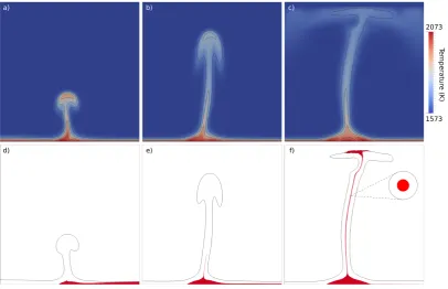
[image:38.595.122.531.55.317.2]

(39)

[image:39.595.124.531.55.317.2]

Figure 2.4: As in Fig. 2.3, but for a case that adopts a concentric plume structure, where B = 0.5, ∆ρc= 0.75%, ˆηc= 1, andδ= 2. Under this scenario, the spatial distribution of geochemical

domains in the lowermost mantle is not preserved during plume ascent.

opposite direction and, consequently, it gradually collects at the foot of the plume. Eventually, this dense material thickens to such an extent that thin tendrils are en-trained into the conduit, with entrainment occurring exclusively within the conduit’s central (hottest) region (Fig. 2.4e). This dense material remains at the conduit’s central axis throughout its ascent to the surface (Fig. 2.4f), thus producing a con-centric conduit structure (Fig. 2.4f, inset). Upon interaction with the overlying lithosphere, dense material spreads laterally to both sides of the domain, which dif-fers from the bilaterally asymmetric cases, where material spreads to one side only (cf. Figs. 2.3f and 2.4f). Under this concentric scenario, the spatial distribution of geochemical domains in the lowermost mantle is not preserved during plume ascent. As a consequence, the distribution of large-scale geochemical heterogeneities in the lowermost mantle cannot be discerned from surface observations. We find that con-centric conduit structures persist at the maximum buoyancy number examined in this study, B = 2, with entrainment rates reduced as B is increased.

3-D Simulations

(40)

[image:40.595.114.539.54.193.2]

Figure 2.5: (a)-(c) temporal snapshots of a 3-D simulation for a case where B = ∆ρc = 0.0,

ˆ

ηc = 1 andδ= 2. The blue isosurface atT = 1823 K outlines the plume, whilst the red isosurface

delineates the reservoir interface at φ= 0.5, which illustrates how bilateral asymmetry develops within the conduit as the simulation evolves.

boundary layer and rises through the mantle with a trailing feeder conduit (Fig. 2.5a/b). As it enters the lower viscosity upper mantle, the head stretches and thins, and eventually impinges on the base of the lithosphere and spreads radially (Fig 2.5c). In 3-D, the chemical reservoir is advected toward the inner conduit, along a radial path. As a result, material from the nearest part of the reservoir is the first to reach the conduit (Fig 2.5b). This material rises up on the proximal side of the conduit only (Fig. 2.5c) and, upon interaction with the base of the lithosphere, spreads only to one side of the conduit and fans out (Fig. 2.6a). This process continues as more and more reservoir material is advected into the conduit’s base. The result is a bilaterally asymmetric plume conduit, which is consistent with our equivalent 2-D case (Fig. 2.3) and with the predictions of previous studies (e.g. Kerr and M´eriaux, 2004; Farnetani and Hofmann, 2010; Farnetani et al., 2012).

Despite differences in material advection into a plume conduit between 2-D and 3-D cases, the effect of varying ∆ρc remains the same: with increasing ∆ρc, reservoir

(41)

[image:41.595.154.496.52.272.2]

Figure 2.6: Snapshots of the two dominant conduit regimes identified in this study. In both cases we plot a blue isosurface atT = 1823 K and the reservoir interface (red) at φ= 0.5. The model parameters are: (a) bilaterally asymmetric: B= ∆ρc= 0.0, ˆηc = 1, andδ= 2; and (b) concentric:

B = 0.5, ∆ρc = 0.75%, ˆηc = 1, and δ = 2. The contrasting distribution of reservoir material

beneath the lithosphere between the two regimes is apparent: only bilaterally asymmetric conduit structures can reliably map the location of the underlying mantle reservoir. For the concentric case, material beneath the lithosphere is dispersed radially and, thus, could have migrated into the conduit’s base along any radial path.

Key Controlling Parameters

The controlling role of the buoyancy number on the evolution of a chemically dense reservoirs has been recognised in previous studies (e.g. van Keken, 1997; Davaille, 1999; Oldham and Davies, 2004; Lin and van Keken, 2006a,b; Deschamps and Tack-ley, 2009). Nonetheless, to illustrate how the effective (local) buoyancy number dictates material transport into mantle plumes, in Fig. 2.7, we plot its variation across the base of the plume conduit that is illustrated in Fig. 2.4. The temper-ature gradient across the conduit, from its hot central axis to its cool periphery, causes a decrease in the effective buoyancy number towards the conduit’s central axis. In other words, the thermal effect on buoyancy is more dominant along the conduit centre and, hence, a plume can preferentially entrain dense material through its core, relative to its periphery. Accordingly, in the presence of significant density contrasts, the final distribution of chemical heterogeneities within a plume conduit will not be indicative of the heterogeneous nature of the plume’s deep-mantle source region.

(42)

viscos-0 60 120 180 240 300 360 420 Radial distance (km)

0 60 120 180 240 300 360 420

Height (km)

0.5 1.0 1.5 2.0

[image:42.595.198.455.56.268.2]

Effective buoyancy number

Figure 2.7: Plot of effective (local) buoyancy number across the base of the plume conduit illustrated in Fig. 2.4. Black lines are temperature contours at T = 1750, 1820, 1890, 1960 and 2040 K. The increased temperature at the conduit centre results in a corresponding decease in effective buoyancy number, illustrating why a plume can more readily sample dense material at its centre relative to its periphery. Note that this plot assumes that dense material, with ∆ρc= 0.75%,

is present everywhere.

ity is increased, concentric structures become more prevalent (Fig. 2.2), since dense material can flow through the lower thermal boundary layer and across the conduit’s central axis more easily. Decreasing (increasing) the dense reservoir’s viscosity fur-ther enhances (discourages) this process and, hence, concentric structures become more (less) likely as ˆηcdecreases (increases). Significantly, the trend towards

concen-tric structures with increasing B and a greater temperature dependence of viscosity is maintained over a broad range of reservoir viscosities.

Implications and Conclusions

Assigning the systematic patterns recorded in the geochemistry of hotspot lavas at Earth’s surface to the heterogeneous structure and composition of Earth’s deep-mantle is an attractive proposition (e.g. Weis et al., 2011; Huang et al., 2011; Far-netani et al., 2012). In this paper we have conducted a systematic 2-D and 3-D analysis of the conditions under which this is possible. Our models are intentionally simple, as our goal is to isolate the effects of chemical density and viscosity contrasts between different chemical domains.

(43)

mantle from being preserved during plume ascent. Given that oceanic crust and primitive iron-rich material, the most likely compositions to be sequestered in the lowermost mantle, are>2% denser than background mantle under deep-mantle con-ditions (e.g. Ringwood, 1975; Stixrude and Lithgow-Bertelloni, 2011), and similar or larger density contrasts are required to form stable, long-lived thermochemical piles (e.g. Tackley, 1998, 2002; McNamara and Zhong, 2004; Deschamps and Tackley, 2009; Davies et al., 2012), we conclude that it is premature to state that the het-erogeneous structure and composition of Earth’s lowermost mantle can be directly mapped from geochemical observations at Earth’s surface (e.g. Weis et al., 2011; Farnetani et al., 2012). Indeed, if deep mantle LLSVPs are interpreted to be dense, stable and long-lived thermochemical piles, our results imply that the scenario pro-posed by Weis et al. (2011), Farnetani et al. (2012) and others (e.g. Huang et al., 2011; Payne et al., 2013; Harpp et al., 2014; Jackson et al., 2014), on the origin of the bilateral asymmetry recorded in Hawaiian and other Pacific hotspot lavas, is invalid: any memory of the spatial distribution of source-region heterogeneities will be lost during plume ascent. The preservation of deep-mantle structure in hotspot lavas is further compounded by: (i) the orientation of a plume conduit relative to plate mo-tion (e.g. Griffiths and Campbell, 1991; Farnetani and Hofmann, 2010; Harpp et al., 2014); and (ii) mixing in magma chambers, which has been shown to dominate the compositional evolution of basaltic melts on Iceland (e.g. Maclennan, 2008; Shorttle et al., 2014).

(44)

of lowermost mantle dynamics (e.g. Schuberth et al., 2009a, 2012; Davies et al., 2012, 2015a). Further testing in global models that account for the effects examined herein, in addition to the complexities arising from subduction, background mantle flow and internal LLSVP structure, will be required to confirm this.

Our study has other important implications: Hofmann and White (1982) first pro-posed the hypothesis that plume related volcanism is derived from a source region that contains recycled oceanic crust. The success of this hypothesis in explaining the geochemistry of ocean island basalts (OIBs) has led to its widespread acceptance. The excess density of oceanic crust means that it should subduct and accumulate in the lowermost mantle, to dominate the primary source region of mantle plumes (e.g. Christensen and Hofmann, 1994; Davies, 2002a; van Keken et al., 2002; Bran-denburg and van Keken, 2007). We offer an additional argument as to why oceanic crust should be a prevalent component in OIBs: the excess density of oceanic crust, which causes it to subduct and sink to the base of the mantle, will also mean that it is preferentially sampled by the centre of plume conduits. Since the conduit centre is also the hottest part of the plume, it is: (i) the most likely part to melt; and (ii) likely to be the dominant source of picrites in plumes that undergo high degrees of partial melting.

(45)

Tungsten Isotopes in Mantle Plumes:

Heads it’s Positive, Tails it’s Negative

T. D. Jones1, D. R. Davies1, P. A. Sossi2

1_{Research School of Earth Sciences, The Australian National University, Canberra, Australia.} 2_{Institut de Physique du Globe, Paris, France}

(46)

Abstract

The lowermost mantle is driven to Earth’s surface by mantle plumes, providing a volcanic record of its structure and composition. Plumes comprise a head and tail, which melt to form large igneous provinces (LIPs) and ocean island basalts (OIBs), respectively. Recent analyses have shown that LIPs and OIBs exhibit tungsten (W) isotope heterogeneity that was created in the first ∼ 60 million years of our solar system’s evolution. Moreover, the isotopic signature found in LIPs differs to that found in OIBs, revealing that the melt products of plume heads must be dominated by a different ancient mantle reservoir to that of plume tails. However, existing geodynamical studies suggest that plume heads and tails sample the same deep-mantle source region and, therefore, cannot account for any systematic differences in composition. Here, we present a suite of numerical simulations of thermo-chemical plumes and an isotopic model for W sources in the mantle. Our results demonstrate that the W isotope systematics of LIPs and OIBs can, under certain conditions, arise as a dynamical consequence of plumes forming in a heterogeneous, thermo-chemical boundary layer. We find that ultra low-velocity zones (ULVZs), which sit on the core-mantle boundary (CMB), likely contribute to the chemical diversity observed in OIBs but not LIPs, while any dense components residing inside large low shear-wave velocity provinces (LLSVPs) may contribute to both. This study places geochemical observations from Earth’s surface in a geodynamically consistent framework and illuminates their relationship with seismically imaged features of the deep mantle.

Introduction

(47)

preferentially partitioned into the metallic core, whilst Hf, as a highly lithophile element, was retained entirely in the silicate mantle. The sensitivity of the 182 Hf-182_{W system to metal-silicate separation has made it a useful chronometer of core} formation in asteroids and the terrestrial planets (e.g. Kleine et al., 2002). This paper focuses on the 182W isotopic anomalies recently identified in materials that make up the silicate Earth (e.g. Rizo et al., 2016b; Mundl et al., 2017a), specifically in volcanic rocks representing the surface expression of mantle plumes: convective instabilities that drive Earth’s lowermost mantle towards its surface (e.g. Morgan, 1971, 1972). As a tectonic plate passes over a plume, its head and tail produce the staggering volume of volcanism associated with Large Igneous Provinces (LIPs) and the far less voluminous and generally age-progressive chain of Ocean Island Basalts (OIBs) that subsequently emerge from them (e.g. Richards et al., 1989).

Basaltic rocks from two LIPs, namely the North Atlantic Igneous Province (NAIP) and the Ontong Java Plateau (OJP), exhibit µ182_{W values (i.e. the deviation of} 182_W/184_{W of a sample from that of a standard in parts per million) ranging from} +10 to +48 (Rizo et al., 2016b), which is considered highly anomalous with respect to the ambient, modern upper mantle value of zero (2σ for Alfa Aesar standard = ±4 ppm: e.g. Mundl et al., 2017a). Conversely, OIBs from Iceland, Hawaii, Samoa

(48)

Insight into the preservation and dynamics of long-lived mantle reservoirs comes from studies of convective mixing (e.g. Sleep, 1988; Christensen and Hofmann, 1994; Kellogg et al., 1999; Becker et al., 1999; Davies, 2002b; Tackley, 2002; Xie and Tackley, 2004; Oldham and Davies, 2004; Huang and Davies, 2007; Brandenburg et al., 2008; Davies et al., 2012; Ballmer et al., 2017). Despite differences between the methods and models used, studies generally agree that to survive billions of years of convective mixing, a reservoir requires sufficient excess compositional den-sity and/or a more-viscous rheology than surrounding mantle. Accordingly, the observed isotopic characteristics of LIPs and OIBs have been linked to seismically defined regions of the lowermost mantle, which may be characterised by excess com-positional density. Specifically, Rizo et al. (2016b) suggest that large low shear-wave velocity provinces (LLSVPs), identified consistently across a number of shear-wave tomography models (e.g. Houser et al., 2008; Ritsema et al., 2011), are a likely source for the positive µ182_{W found in LIPs. This hypothesis makes two central} assumptions: (i) that LLSVPs represent long-lived chemically distinct structures, termed thermo-chemical ‘piles’ (e.g. Tackley, 1998; McNamara and Zhong, 2005; Bower et al., 2013); and (ii) that any dense material residing inside LLSVPs can be transported into and preserved within a plume head, as the plume rises from the deep-mantle to Earth’s surface. Furthermore, Mundl et al. (2017a) hypothesise that so called ‘mega’ ultra-low velocity zones (ULVZs) (e.g. Cottaar and Romanowicz, 2012; Thorne et al., 2013; Yuan and Romanowicz, 2017) are a likely reservoir for the negativeµ182_{W found in OIBs, a hypothesis that relies on similar assumptions.} The thermo-chemical structure and origin of both LLSVPs and ULVZs remains un-clear, with recent debate focusing upon the length-scale, dynamical significance and radial extent of any compositionally distinct material residing inside LLSVPs (see Davies et al., 2015a; McNamara, 2018, for recent reviews). In addition, the dynam-ical feasibility of the Rizo et al. (2016b) and Mundl et al. (2017a) hypotheses, when considered in isolation or simultaneously, have not yet been demonstrated. Doing so necessitates a quantitative understanding of the interaction between mantle plumes and deep-mantle compositional heterogeneity.

(49)

ap-pears systematic and, therefore, the result of a common process that causes the melt products of plume heads and tails to exhibit different average isotopic charac-teristics. Early laboratory experiments seemed to offer a simple explanation. The laboratory plume models of Griffiths and Campbell (1990) produced plume heads that entrain the surrounding mantle as they ascend, becoming a mixture of mate-rial from within the thermal boundary layer (TBL) and overlying ambient mantle, whereas TBL material ascending through a plume tail would undergo little contam-ination from entrained ambient mantle. Thus, the experiments predicted that the composition of plume heads would consistently diverge from their tails. However, more recent laboratory and numerical studies, which trace the material origin of plumes, demonstrate that entrainment by plume heads is minimal and, more im-portantly, entrained material does not approach the melt region that feeds surface volcanism (e.g. Farnetani and Richards, 1995; Lohmann et al., 2009). Farnetani and Richards (1995) conclude that the compositional differences between plume heads and tails reflects either inherent source region heterogeneity or contamination from the crust and lithosphere. Lohmann et al. (2009), on the other hand, favour a dif-ferential melting hypothesis, whereby LIPs and OIBs reflect melting of the same heterogeneous source to a higher versus lower degree, respectively. Neither crustal contamination or differential melting have been shown to explain the isotopic differ-ences between LIPs and OIBs and, furthermore, source region heterogeneity alone offers no explanation for a systematic contrast between the two.

In this paper we provide an alternative explanation based upon the predictions of numerical simulations that examine the interaction between mantle plumes and deep-mantle compositional heterogeneity. Fluid dynamics calculations and labora-tory experiments show that the dynamical requirements of plume formation cause their heads to be more voluminous, and thus more buoyant, than their tails (e.g. Selig, 1965; Whitehead and Luther, 1975). This, we demonstrate, allows plume heads to entrain dense components of the mantle that their tails leave behind, set-ting up a dynamical system whereby LIPs and OIBs consistently diverge in source composition.

(50)

described in Section 3, highlight general characteristics of thermo-chemical mantle plumes, alongside the factors controlling their structure and dynamics, and demon-strate the dynamical feasibility of the hypotheses proposed by Rizo et al. (2016b) and Mundl et al. (2017a) within a limited parameter space. In Section 4, we for-mulate an isotopic model of W sources in the mantle and determine the degree of mixing required to produce values ofµ182_{W that fall within the observed range (Rizo} et al., 2016b; Mundl et al., 2017a). The degree of mixing implied by these calcula-tions constrains the set of our thermo-chemical plume models that can account for the observed range ofµ182W values as a function of source variation alone, which we summarise through a regime diagram. We conclude by discussing the implications of our results for the thermo-chemical structure of Earth’s deep mantle, as well as the limitations of our study and avenues for future research.

Methodology

We solve the equations governing mantle convection (conservation of mass, momen-tum and energy) using Fluidity (e.g. Davies et al., 2011; Kramer et al., 2012; Le Voci et al., 2014), a finite-element, control-volume computational modelling framework. We also solve for a volume fraction field that tracks the presence of distinct chemical regions. To avoid numerical diffusion, this is discretized on a control volume mesh, using the minimally diffusive HyperC face-value scheme (see Wilson, 2009; Garel et al., 2014, for further details). Our simulations exploit an adaptive, unstructured mesh, providing increased resolution in regions of dynamic importance (i.e. at the interface between materials and in regions of strong temperature, velocity and vis-cosity contrasts), with minimum and maximum element sizes of 0.5 and 25 km, respectively.

(51)

background mantle, dense material and ultra-dense material, with the latter initiated as a thin layer at the very base of the model, approximating ULVZ material that sits at the core-mantle-boundary. In all results that follow, we refer to the dense material residing inside LLSVPs asdense, and the ultra-dense material representing ULVZs asultra-dense.

Key model parameters are provided in Table 3.1. Simulations are undertaken in a 2-D square domain of dimensions 2900×2900 km. Boundary conditions for tem-perature are T = 273 K at the surface, T = 2073 K at the base, with insulating (homogeneous Neumann) side-walls. Velocity boundary conditions are free-slip and no normal flow at all boundaries. The material volume fraction, φ, is set to 1 inside a layer at the base of the domain and 0 elsewhere. For two component models we examine cases with an initial dense layer of thickness, hc = 50, 75, 125 and 200

km. For three component models we examine only the case where hc = 65 km with

an additional ultra-dense layer of 10 km thickness. For each model we specify the buoyancy number:

B = ∆ρc ρ0α∆T

(3.1)

which denotes the ratio of the (stabilising) chemical density contrast, ∆ρc, to the

(destabilising) thermal density contrast (∆T = TCM B − Tp = 500 K). For two

component models, we examine simulations for cases where B ranges from 0.0 to 1.0, in increments of 0.1, for each value ofhc. For three component models,B = 0.6

for dense material and B = 6.6 for ultra-dense material. A temperature dependent viscosity is used following the relation:

η(T∗) =η0exp−bT ∗

(3.2) where T∗ = (T −TS)/(TCM B −TS) is the non-dimensionalised temperature. The

reference viscosity, η0, is multiplied by ˆη660 below 660 km depth and ˆηlith for

tem-peratures below 1573 K. The temperature dependence of viscosity is controlled by b = ln(10δ), where δ = 3 for all simulations examined herein.

Models are initiated with a 150 km thick TBL at the base, defined via an error function, where temperature ranges from Tp = 1573 K toTCM B = 2073 K. We take