Cloud Technologies for Bioinformatics Applications

Cloud Technologies for Bioinformatics

Applications

Jaliya Ekanayake, Thilina Gunarathne, Judy Qiu

Abstract—Executing large number of independent jobs or jobs comprising of large number of tasks that perform minimal inter-task communication is a common requirement in many domains. Various technologies ranging from classic job schedulers to the latest cloud technologies - such as MapReduce - can be used to execute these “many-tasks” in parallel. In this paper, we present our experience in applying two cloud technologies - Apache Hadoop and Microsoft DryadLINQ - to two bioinformatics applications with the above characteristics. The applications are a pairwise Alu sequence alignment application and an EST (Expressed Sequence Tag) sequence assembly program. First, we compare the performance of these cloud technologies using the above applications and also compare them with traditional MPI implementation in one application. Next, we analyze the effect of inhomogeneous data on the scheduling mechanisms of the cloud technologies. Finally, we present a comparison of performance of the cloud technologies under virtual and non-virtual hardware platforms.

Index Terms—Distributed Programming, Parallel Systems, Performance, Programming Paradigms.

——————————  ——————————

1

I

HERE is increasing interest in approaches to data analysis in scientific computing as essentially every field is seeing an exponential increase in the size of the data deluge. The data sizes imply that parallelism is es-sential to process the information in a timely fashion. This is generating justified interest in new runtimes and pro-gramming models that, unlike traditional parallel models (such as MPI), directly address the data-specific issues. Experience has shown that the initial (and often most time consuming) parts of data analysis are naturally data parallel and the processing can be made independent with perhaps some collective (reduction) operation. This structure has motivated the important MapReduce [1] paradigm and many follow-on extensions. Here we exam-ine two technologies (Microsoft Dryad/DryadLINQ [2][3] and Apache Hadoop [4]) on two different bioinformatics applications (EST [5][6] and Alu clustering [7][8]) and for the later we also present details of an MPI implementa-tion as well. Dryad is an implementaimplementa-tion of extended MapReduce from Microsoft. All the applications are (as is often so in Biology) ―doubly data parallel‖ (or ―all pairs‖ [9]) as the basic computational unit is replicated over all pairs of data items from the same (in our cases) or differ-ent datasets. In the EST example, each parallel task exe-cutes the CAP3 program on an input data file inde-pendently of others and there is no ―reduction‖ or ―ag-gregation‖ necessary at the end of the computation. On

the other hand, in the Alu case, a global aggregation is necessary at the end of the independent computations to produce the resulting dissimilarity matrix. In this paper, we evaluate different technologies showing that they give comparable performance despite their different pro-gramming models.

1.1 Cloud and Cloud Technologies

Cloud and cloud technologies are two broad categories of technologies related to the general notion of Cloud Com-puting. By ―Cloud,‖ we refer to a collection of infrastruc-ture services such as Infrastrucinfrastruc-ture-as-a-service (IaaS), Platform-as-a-Service (PaaS), etc., provided by various organizations where virtualization usually plays a key role. By ―Cloud Technologies,‖ we refer to various cloud runtimes such as Hadoop, Dryad and other MapReduce frameworks, and also the storage and communication frameworks such as Hadoop Distributed File System (HDFS), Amazon S3, etc. Although we name them as cloud technologies, runtimes such as Hadoop and Dryad can be run on local resources as well.

1.2 Relevance of MapReduce to Many Task Computing

MapReduce programming model comprises of two com-putation steps (map/reduce) and an intermediate data shuffling step, which can be used to implement many parallel applications. The three steps collectively provide functionality beyond the requirements of simple many task computations (MTC). However, this does not hinder the usability of MapReduce to MTC applications. For ex-ample, when only a map operation is used, the MapRe-duce programming model reMapRe-duces to a ―map-only‖ ver-sion that is an ideal match for MTC applications. Fur-thermore, with the capability of adding a ―reduction‖

xxxx-xxxx/0x/$xx.00 © 200x IEEE Manuscript received (insert date of submission if desired).

T

————————————————

 Jaliya Ekanayake, Thilina Gunarathne, and Judy Qiu are with School of Informatics and Computing and Pervasive Technology Institute of Indiana University, Bloomington, IN 47408. E-mail: jekanaya@cs.indiana.edu, tgunarat@indiana.edu, xqiu@indiana.edu.

operation MapReduce can be used to collect or merge results of an embarrassingly parallel phase of some of the MTC applications as well. Our research on applying MapReduce to many task computations was motivated by these observations.

In section 2, we give a brief introduction to the two cloud technologies we used while the applications, EST and Alu sequencing are discussed in section 3. Section 4 presents some performance results. Conclusions are given in section 7 after a discussion of the different program-ming models in section 5 and related work in section 6.

2

C

T

Dryad is a distributed execution engine for coarse grain data parallel applications. It combines the MapReduce programming style with dataflow graphs to solve the computation tasks. Dryad considers computation tasks as directed acyclic graph (DAG) where the vertices represent computation tasks and with the edges acting as communi-cation channels over which the data flow from one vertex to another. The data is stored in (or partitioned to) local disks via the Windows shared directories and meta-data files and Dryad schedules the execution of vertices de-pending on the data locality. (Note: The academic release of Dryad only exposes the DryadLINQ API for program-mers [3][10]. Therefore, all our implementations are writ-ten using DryadLINQ although it uses Dryad as the un-derlying runtime). Dryad stores the output of vertices in local disks, and the other vertices which depend on these results, access them via the shared directories. This ena-bles Dryad to re-execute failed vertices, a step which im-proves fault tolerance of the programming model. The current academic release of DryadLINQ runs only on the Windows HPC Server 2008 operation system.

2.2 Apache Hadoop

Apache Hadoop has a similar architecture to Google’s MapReduce[1] runtime. Hadoop accesses data via HDFS [4], which maps all the local disks of the compute nodes to a single file system hierarchy, allowing the data to be dispersed across all the data/computing nodes. HDFS also replicates the data on multiple nodes so that failures of nodes containing a portion of the data will not affect the computations which use that data. Hadoop schedules the MapReduce computation tasks depending on the data locality, improving the overall I/O bandwidth. The out-puts of the map tasks are stored in local disks until the

reduce tasks access them (pull) via HTTP connections. Although this approach simplifies the fault handling mechanism in Hadoop, it adds a significant communica-tion overhead to the intermediate data transfers, especial-ly for applications that produce small intermediate results frequently. Apache Hadoop runs only on Linux operating systems.

3

A

3.1 Alu Sequence Classification

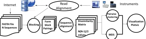
The Alu clustering problem [8] is one of the most chal-lenging problems for sequence clustering because Alus represent the largest repeat families in human genome. There are about 1 million copies of Alu sequences in hu-man genome, in which most insertions can be found in other primates and only a small fraction (~ 7000) is hu-man-specific. This indicates that the classification of Alu repeats can be deduced solely from the 1 million human Alu elements. Alu clustering can be viewed as a classical case study for the capacity of computational infrastruc-tures because it is not only of great intrinsic biological interest, but also a problem of a scale that will remain as the upper limit of many other clustering problems in bio-informatics for the next few years, such as the automated protein family classification for millions of proteins. In our previous works we have examined Alu samples of 35339 and 50,000 sequences using the pipeline of figure 1.

Fig. 1. Pipeline for analysis of sequence data.

3.1.1 Complete Alu Application

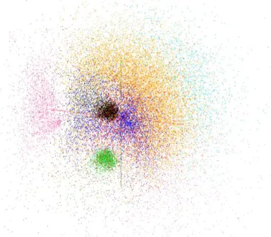
This application uses two highly parallel traditional MPI applications, i.e. MDS (Multi-Dimensional Scaling) and Pairwise (PW) Clustering algorithms described in Fox, Bae et al. [7]. The latter identifies relatively isolated se-quence families as shown in the example depicated in figure 2. MDS allows visualization by mapping the high dimension sequence data to lower (in our case 3) dimen-sionfor visualization. MDS finds the best set of 3D vec-tors x(i) such that a weighted least squares sum of the difference between the sequence dissimilarity D(i,j) and the Euclidean distance |x(i) - x(j)| is minimized. This has a computational complexity of O(N2_{) to find 3N} un-knowns for N sequences.

The PWClustering algorithm is an efficient MPI paral-lelization of a robust EM (Expectation Maximization) method using annealing (deterministic not Monte Carlo) originally developed by Ken Rose, Fox [14, 15] and others [16]. This improves over other clustering methods, such as Kmeans, which are sensitive to false minima. The orig-inal clustering work was based on a vector space model (like Kmeans) where a cluster is defined by a vector as its center. However, in a major advance 10 years ago [16], it was shown how one could use a vector free approach and operate with just the distances D(i,j). This method is clear-ly the most natural for problems like Alu sequence anaclear-ly- analy-sis where current global sequence alignment approaches (over all N sequences) are problematic, but D(i,j) can be precisely calculated for each pair of sequences. PWClus-tering also has a time complexity of O(N2_{) and in practice} we find all three steps (Calculate D(i,j), MDS and Visualization

Plotviz Blocking _alignmentSequence

FASTA File N Sequences

Form block Pairings

Internet Read Alignment

Instruments

MDS Pairwise clustering Dissimilarity

Matrix

PWClustering) take comparable times (a few hours for 50,000 sequences on 768 cores) although searching for a large number of clusters and refining the MDS can in-crease their execution time significantly. We have pre-sented performance results for MDS and PWClustering elsewhere [7][12] and for large data sets the efficiencies are high (showing sometimes super linear speed up). In the rest of the paper, we only discuss the initial dissimi-larity computation.

Fig. 2. Display of Alu clusters from MDS and clustering calculation from 35339 sequences using SW-G distances. The clusters corre-sponding to younger families AluYa, AluYb are particularly tight.

As shown in figure 1, the initial step of the pipeline is to compute the pairwise dissimilarities between each pair of genes in the data set. Since the comparison happens with the same set of genes, effectively we only need to perform half of the computations. However, the latter two stages (Clustering and MDS) require the output of the first stage to be in a format appropriate for the later MPI-based data mining stages. The MDS and PWClustering algorithms require a particular parallel decomposition where each of N processes (MPI processes, threads) has 1/N of sequences and for this subset {i} of sequences stores in memory D({i},j) for all sequences j and the subset {i} of sequences for which this node is responsible. This implies that often we need D(i,j) and D(j,i) (which are equal) stored in different processors/disks. We designed our initial calculation of D(i,j) so that we only calculated the independent set, but the data was stored so that the later MPI jobs could access the data needed.

3.1.2 Smith Waterman Dissimilarities

We identified samples of the human and Chimpanzee Alu gene sequences using Repeatmasker [13] with Rep-base Update [14]. We used an open source implementa-tion, named NAligner[11], of the Smith Waterman – Gotoh algorithm SW-G [15][16] modified to ensure low start up effects by each thread, processing a large number (above a few hundred) of sequence calculations at a time. Memory bandwidth needed was reduced by storing data items in as few bytes as possible. In the following two sections, we discuss the efficient usage of MapReduce,

DryadLINQ and MPI for the the initial phase of calculat-ing distances D(i,j) for each pair of sequences.

3.1.3 Parallelizing SW-G as a Many Task Computation

In this section, we discuss two approaches to partition the workload of the SW-G application as a many task compu-tation. Both these approaches use block based coarse grain task decomposition to minimize task scheduling overheads as individual comparisons take significantly less time.

Fig. 3. Two task decomposition approaches considering the final output as a block matrix. (Top) using only the upper triangle of the output matrix, (Bottom) using the symmetry of the calculations.

3.1.4 First Approach: Considering the Upper Triangular (TU) Blocks

In this approach, the overall pairwise computation is de-composed into tasks by considering the output matrix. To clarify our algorithm, let’s consider an example where N gene sequences produce a pairwise distance matrix of size NxN. We decompose the computation task by consider-ing the resultant matrix and group the overall computa-tion into a block matrix of size DxD where D is a multiple (>2) of the available computation nodes and d=(N/D). Due to the symmetry of the distances D(i,j) and D(j,i), we only calculate the distances in the blocks of the upper triangle of the block matrix as shown in figure 3 (top). Diagonal blocks are specially handled and calculated as full sub blocks. As the number of diagonal blocks is D and total number is D(D+1)/2, there is no significant

1 (1-100)

2 (101-200)

3 (201-300)

4 (301-400)

N

1

(1-100) M1 M2

from

M6 M3 …. M#

Reduce 1 hdfs://.../rowblock_1.out

2 (101-200)

from

M2 M4 M5

from

M9 ….

Reduce 2 hdfs://.../rowblock_2.out

3 (201-300) M6

from

M5 M7 M8 ….

Reduce 3 hdfs://.../rowblock_3.out

4 (301-400)

from

M3 M9

from

M8 M10 ….

Reduce 4 hdfs://.../rowblock_4.out

. . . .

. . . .

. . . .

. . . .

…. …. …. ….

. . . . N From

M#

M(N* (N+1)/2)

Reduce N hdfs://.../rowblock_N.out 0

..

..

(0,d-1) (0,d-1)

Upper triangle

0

1

2

D-1

0 1 2 D-1

NxN matrix broken down to DxD blocks

Blocks in lower triangle are not calculated directly

0

(0,2d-1) (0,d-1)

0 ((D-1)d,Dd-1)D-1 (0,d-1)

D

(0,d-1) (d,2d-1)

D+1

(d,2d-1) (d,2d-1)

((D-1)d,Dd-1) ((D-1)d,Dd-1)

compute overhead added. Once the block boundaries are defined, the upper triangular blocks are processed sepa-rately resembling a MTC application. Each UT block pro-duces two outputs; (i) the pairwise distances correspond-ing to the genes in the block’s boundary and (ii) the transpose of the same to represent the corresponding un-calculated block in the lower triangle. The diagonal blocks do not produce duplicates as both the output and the transpose are the same.

3.1.5 Second Approach: Considering the Symmetry of Blocks

A load balanced task partitioning strategy for all pairs problems can be devised using the following rules, which we use to identify the blocks that need to be computed as shown in the figure 3 (bottom). In addition, similar to the first partitioning appraoch, all the blocks in the diagonal needs to be computed due to the usage of blocks. Except for the diagonal blocks, all the other computation blocks produce distances for itself and transpose.

When β >= α, we calculate D(α,β) only if α+β is even, When β < α, we calculate D(α,β) only if α+β is odd. Irrespective of the adopted decomposition approache, the pairwise SW-G calculations yield the same amount of calculations in both approaches and they both can be exe-cuted as a MTC application. Next we will discuss how we map these algorithms to different runtimes.

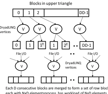
Fig. 4. DryadLINQ implementation of SW-G pairwise distance calcu-lation.

3.1.6 DryadLINQ Implementation

We used DryadLINQ’s ―Apply‖ operation to execute a function to calculate (N/D)x(N/D) distances in each block. The function internally uses the NAligher (C# ver-sion of JAligner[20]) library to calculate SW-G dissimilari-ty for each pair of genes. After computing the distances in each block, the function calculates the transpose matrix of the result matrix which corresponds to a block in the low-er triangle, and writes both these matrices into two out-put files in the local file system. The names of these files and their block numbers are communicated back to the

main program. The main program sorts the files based on their block numbers and performs another ―Apply‖ oper-ation to combine the files corresponding to rows in block matrix as shown in the figure 4. The first step of this com-putation dominates the overall running time of the appli-cation, and with the algorithm explained it clearly resem-bles the characteristics of a ―many-task‖ problem.

3.1.7 Hadoop Implementation

We developed an Apache Hadoop version of the pairwise distance calculation program based on the JAligner[20] program - the java implementation of the NAligner used in the Dryad implementation. Similar to the other im-plementations, the computation is partitioned into blocks based on the resultant distance matrix. Each of the blocks would get computed as a map task. The block size (D) can be specified via an argument to the program. The block size needs to be specified in such a way that there will be much more map tasks than the map task capacity of the system, so that the Apache Hadoop scheduling will happen as a pipeline of map tasks resulting in global load balancing inside the application. The input data is distributed to the worker nodes through the Hadoop dis-tributed cache, which makes them available in the local disk of each compute node. Hadoop uses the block sym-metry based second partitioning approach we described above to identify the blocks to compute.

The figure 5 depicts the run time behavior of the Ha-doop SW-G program. In the given example the map task capacity of the system is ―k‖ and the number of blocks is ―N‖. The solid black lines represent the starting state, where ―k‖ map tasks corresponding to ―k‖ computation blocks will get scheduled in the compute nodes. The dashed black lines represent the state at time t1 , when 2 map tasks, m2 & m6, get completed and two map tasks from the pipeline get scheduled for the placeholders emp-tied by the completed map tasks. The gray dotted lines represent the future.

Map tasks use custom Hadoop writable objects as the map task output values to store the calculated pairwise distance matrices for the respective blocks. In addition, non-diagonal map tasks output the inverse of the distanc-es matrix of the block as a separate output value. Hadoop uses local files and http transfers to transfer the map task output key-value pairs to the reduce tasks.

The outputs of the map tasks are collected by the re-duce tasks. Since the rere-duce tasks start collecting the map task outputs as soon as the first map task completes the execution and continue to do so while other map tasks are executing, the data transfers from the map tasks to reduce tasks do not present a significant performance overhead to the program ue to the overlapping of computation with I/O. The program currently creates a single reduce task per each row block resulting in total of (no. of sequenc-es/block size) Reduce tasks. Each reduce task accumu-lates the output distances for a row block and writes the collected output to a single file in Hadoop Distributed File System (HDFS). This results in N number of output files corresponding to each row block, similar to the

out-0 1 DD-1

V V V

..

..

V V V

..

DryadLINQ vertices

File I/O DryadLINQ

vertices

Each D consecutive blocks are merged to form a set of row blocks each with NxD elementsprocess has workload of NxD elements

Blocks in upper triangle

0 1 1T _{1 2}T _DD-1 V

2

put we produce in the Dryad version.

Fig. 5. Hadoop implementation SW-G pairwise distance calculation application.

3.1.8 MPI Implementation

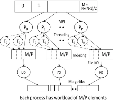
The MPI version of SW-G calculates pairwise distances using a set of either single or multi-threaded processes. For N gene sequences, we need to compute half of the values (in the lower triangular matrix), which is a total of M = N x (N-1) /2 distances. At a high level, computation tasks are evenly divided among P processes and execute in parallel. Namely, computation workload per process is M/P. At a low level, each computation task can be fur-ther divided into subgroups and run in T concurrent threads. Our implementation is designed for flexible use of shared memory multicore system and distributed memory clusters (tight to medium tight coupled commu-nication technologies such threading and MPI). We pro-vide options for any combinations of thread vs. process vs. node, but in earlier papers [7][12] we have shown that threading is much slower than MPI for this class of prob-lems.

Fig. 6. MPI implementation SW-G pairwise distance calculation ap-plication

We have implemented the above blocked algorithm in

MPI as well. Points are divided into blocks such that each processor is responsible for all blocks in a simple decom-position illustrated in the figure 6. This also illustrates the initial computation, where to respect symmetry, we calcu-late half the D(,) using the same criterion used in Ha-doop implementation:

This approach can be applied to points or blocks. In our implementation, we applied it to blocks of points -- of size (N/P)x(N/P) where we use P MPI processes. Note we get better load balancing than the ―Space Filling‖ al-gorithm as each processor samples all values of . This computation step must be followed by a communication step illustrated in figure 6 which gives full strips in each process. The latter can be straightforwardly written out as properly ordered file(s).

3.1.9 Discussion

Although the above three implementations use almost the same algorithm for the SW-G problem, depending on the runtime used we were forced to use some of the runtime features when implementing them. For example, in Ha-doop, the data is read from its distributed file system HDFS while we used local disks in DryadLINQ and for MPI. Similarly, the different runtimes follow different task scheduling approaches as well. In MPI, the tasks are statically scheduled to the available CPU cores. Dry-adLINQ schedules tasks to the computation nodes stati-cally but internal to nodes, the tasks are scheduled to dif-ferent CPU cores dynamically. Hadoop on the other hand schedules tasks to CPU cores dynamically. These differ-ences contributed to different runtime performances. However, our motivation in this paper is to demonstrate the applicability of these runtimes to two biology applica-tions that represent the class of ―many task‖ computa-tions and discuss the performance characteristics one may get in using them.

3.2 CAP3 Application EST and Its Software CAP3

3.2.1 EST and Its Software CAP3

An EST (Expressed Sequence Tag) corresponds to mes-senger RNAs (mRNAs) transcribed from the genes resid-ing on chromosomes. Each individual EST sequence rep-resents a fragment of mRNA, and the EST assembly aims to re-construct full-length mRNA sequences for each ex-pressed gene. Because ESTs correspond to the gene re-gions of a genome, EST sequencing has become a stand-ard practice for gene discovery, especially for the ge-nomes of many organisms that may be too complex for whole-genome sequencing. EST is addressed by the soft-ware CAP3 which is a DNA sequence assembly program developed by Huang and Madan [17]. CAP3 performs several major assembly steps including computation of overlaps, construction of contigs, construction of multiple sequence alignments, and generation of consensus se-quences to a given set of gene sese-quences. The program reads a collection of gene sequences from an input file (FASTA file format) and writes its output to several out-M =

0 1 _Nx(N-1)/2

P0 P1

..

..

T0

M/P M/P M/P

T0 T0 T0 T0 T0

I/O I/O I/O

..

Merge files File I/O MPI

Threading

put files, as well as the standard output.

CAP3 is often required to process large numbers of FAS-TA formatted input files, which can be processed inde-pendently, making it an embarrassingly parallel applica-tion requiring no inter-process communicaapplica-tions. We have implemented a parallel version of CAP3 using Hadoop and DryadLINQ. In both these implementations we adopt the following algorithm to parallelize CAP3.

1. Distribute the input files to storages used by the runtime. In Hadoop, the files are distributed to HDFS and in DryadLINQ the files are distributed to the in-dividual shared directories of the computation nodes 2. Instruct each parallel process (in Hadoop these are

the map tasks and in DryadLINQ these are the verti-ces) to execute CAP3 program on each input file. This application resembles a common parallelization requirement, where an executable, a script, or a function in a special framework such as Matlab or R, needs to be applied on a collection of data items. We can develop DryadLINQ & Hadoop applications similar to the CAP3 implementations for all these use cases. One can use MPI to implement a parallel version of CAP3. However, then the application needs to handle initial file distribution and final results collection manually. Since CAP3 is exe-cuted as a standalone application by each parallel process in MPI, even with the above extra work it would not yield any performance gains. Therefore we did not implement CAP3 using MPI but rather focused on Hadoop and Dry-adLINQ.

3.2.2 DryadLINQ Implementation

As discussed in section 3.2.1 CAP3 is a standalone execut-able that processes a single file containing DNA sequenc-es. To implement a parallel CAP3 application using Dry-adLINQ we adopted the following approach: (i) the input files are partitioned among the nodes of the cluster so that each node of the cluster stores roughly the same number of input files; (ii) a ―data-partition‖ (A text file for this application) is created in each node containing the names of the input files available in that node; (iii) a DryadLINQ ―partitioned-file‖ (a meta-data file understood by Dry-adLINQ) is created to point to the individual data-partitions located in the nodes of the cluster. These three steps enable DryadLINQ programs to execute queries against all the input data files. Once this is done, the Dry-adLINQ program which performs the parallel CAP3 exe-cution is just a single line program contacting a ―Select‖ query which select each input file name from the list of file names and execute a user defined function on that. In our case, the user defined function calls the CAP3 pro-gram passing the input file name as propro-gram arguments. The function also captures the standard output of the CAP3 program and saves it to a file. Then it moves all the output files generated by CAP3 to a predefined location.

3.2.3 Hadoop Implementation

Parallel CAP3 sequence assembly fits as a ―map only‖ application for the MapReduce model. The Hadoop ap-plication is implemented by writing map tasks which

ex-ecute the CAP3 program as a separate process on a given input FASTA file. Since the CAP3 application is imple-mented in C, we do not have the luxury of using the Ha-doop file system (HDFS) directly from the program. Hence the individual data files are downloaded to the nodes using a custom Hadoop InputFormat and a custom RecordReader, while preserving the data locality needs to be stored in a shared file system across the nodes.

4

P

In this section we study the performance of SW-G and CAP3 applications under increasing homogeneous work-loads, inhomogeneous workloads with different standard deviations and the performance in cloud like virtual envi-ronments. A 32 nodes IBM iDataPlex cluster, with each node having 2 quad core Intel Xeon processors (total 8 cores per node) and 32 GB of memory per node was used for the performance analysis under the following operat-ing conditions: (i) Microsoft Window HPC Server 2008, service Pack 1 - 64 bit; (ii) Red Hat Enterprise Linux Serv-er release 5.3 -64 bit on bare metal; and (iii) Red Hat En-terprise Linux Server release 5.3 -64 bit on Xen hypervisor (version 3.0.3).

In our performance measures we are focusing on DryadLINQ and Hadoop and the various performance issues that one would encounter in using these runtimes. The two runtimes does not provide identical interfaces and therefore we had to use different features depending on the runtime. For example, in DryadLINQ the files are accessed from shared directories while Hadoop uses HDFS. Further, Hadoop only runs on Linux while Dry-adLINQ require Windows HPC Server 2008. Apart from the above, we could not use DryadLINQ for the study of the performance implications of virtualization simply because the Windows HPC Server 2008 is not yet availa-ble for XEN. However, our motivation in this research is to develop and deploy applications using the best strate-gy for each runtime and analyze their performances to see what benefits one can gain from using these cloud tech-nologies.

4.1 Scalability of different implementations

4.1.1 SW-G

Jaligner on Linux in the hardware we used for the per-formance analysis.

The results for this experiment are given in the figure 7. The time per actual calculation is computed by dividing the total time to calculate pairwise distances for a set of sequences by the actual number of comparisons per-formed by the application. According to figure 7, all three implementations perform and scale satisfactorily for this application with Hadoop implementation showing the best scaling. As expected, the total running times scaled proportionally to the square of the number of sequences. The Hadoop & Dryad applications perform and scale competitively with the MPI application.

Fig. 7. Scalability of Smith Waterman pairwise distance calculation applications.

Fig. 8. Scalability of Cap3 applications.

We can notice that the performance of the Hadoop im-plementation improving with the increase of the data set size, while Dryad performance degrades a bit. Hadoop improvements can be attributed to the diminishing of the framework overheads, while the Dryad degradation can be attributed to the memory management issues in the Windows and Dryad environment.

4.1.2 CAP3

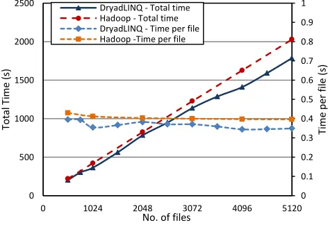
We analyzed the scalability of DryadLINQ & Hadoop implementations of the CAP3 application with the

in-crease of the data set using homogeneous data sets. We prepare the data sets by replicating a single fasta file to represent a uniform workload across the application. The selected fasta sequence file contained 458 sequences.

The results are shown in the figure 8. The primary ver-tical axis (left) shows the total time vs. the number of files. Secondary axis (right) shows the time taken per file (total time / number of files) against the number of files. Both the DryadLINQ and Hadoop implementations show good scaling for the CAP3 application, although Dryad's scaling is not as smooth as the Hadoop scaling curve. Standalone CAP3 application used as the kernel for these applications performs better in the windows environment than in the Linux environment, which must be contrib-uting to the reason for Hadoop being slower than Dryad.

4.2 Inhomogeneous Data Analysis

New generation parallel data processing frameworks such as Hadoop and DryadLINQ are designed to perform optimally when a given job can be divided in to a set of equally time consuming sub tasks. Most of the data sets we encounter in the real world however are inhomogene-ous in nature, making it hard for the data analyzing pro-grams to efficiently break down the problems in to equal sub tasks. At the same time we noticed Hadoop & Dry-adLINQ exhibit different performance behaviors for some of our real data sets. It should be noted that Hadoop & Dryad uses different task scheduling techniques, where Hadoop uses global queue based scheduling and Dryad uses static scheduling. These observations motivated us to study the effects of data inhomogeneity in the applica-tions implemented using these frameworks.

4.2.1 SW-G Pairwise Distance Calculation

The inhomogeneity of data applies for the gene sequence sets too, where individual sequence lengths and the con-tents vary among each other. In this section we study the effect of inhomogeneous gene sequence lengths for the performance of our pairwise distance calculation applica-tions.

𝑆𝑊𝐺(𝐴, 𝐵) = 𝑂(𝑚𝑛)

The time complexity to align and obtain distances for two genome sequences A, B with lengths m and n respectively using Smith-Waterman-Gotoh algorithm is approximate-ly proportional to the product of the lengths of two se-quences (O(mn)). All the above described distributed im-plementations of Smith-Waterman similarity calculation mechanisms rely on block decomposition to break down the larger problem space in to sub-problems that can be solved using the distributed components. Each block is assigned two sub-sets of sequences, where Smith-Waterman pairwise distance similarity calculation needs to be performed for all the possible sequence pairs among the two sub sets. According to the above mentioned time complexity of the Smith-Waterman kernel used by these distributed components, the execution time for a particu-lar execution block depends on the lengths of the se-quences assigned to the particular block.

0.000 0.005 0.010 0.015 0.020 0.025

10000 20000 30000 40000

Ti

m

e

p

er

A

ct

ua

l Cal

cul

at

io

n

(m

s)

No. of Sequences

Hadoop SW-G MPI SW-G DryadLINQ SW-G

0 0.1 0.2 0.3 0.4 0.5 0.6 0.7 0.8 0.9 1

0 500 1000 1500 2000 2500

0 1024 2048 3072 4096 5120

Ti

m

e

pe

r

fi

le

(

s)

To

tal

T

im

e (

s)

No. of files

Parallel execution frameworks like Dryad and Hadoop work optimally when the work is equally partitioned among the tasks. Depending on the scheduling strategy of the framework, blocks with different execution times can have an adverse effect on the performance of the applica-tions, unless proper load balancing measures have been taken in the task partitioning steps. For an example, in Dryad vertices are scheduled at the node level, making it possible for a node to have blocks with varying execution times. In this case if a single block inside a vertex takes a longer amount of time than other blocks to execute, then the entire node must wait until the large task com-pletes, which utilizes only a fraction of the node re-sources.

Fig. 9. Performance of SW-G pairwise distance calculation applica-tion for randomly distributed inhomogeneous data with „400‟ mean sequence length.

For the inhomogeneous data study we decided to use controlled inhomogeneous input sequence sets with same average length and varying standard deviation of lengths. It’s hard to generate such controlled input data sets using real sequence data as we do not have control over the length of real sequences. At the same time we note that the execution time of the Smith-Waterman pairwise dis-tance calculation depends mainly on the lengths of the sequences and not on the actual contents of the sequenc-es. This property of the computation makes it possible for us to ignore the contents of the sequences and focus only on the sequence lengths, thus making it possible for us to use randomly generated gene sequence sets for this ex-periment. The gene sequence sets were randomly gener-ated for a given mean sequence length (400) with varying standard deviations following a normal distribution of the sequence lengths. Each sequence set contained 10000 sequences leading to 100 million pairwise distance calcu-lations to perform. We performed two studies using such inhomogeneous data sets. In the first study the sequences with varying lengths were randomly distributed in the data sets. In the second study the sequences with varying lengths were distributed using a skewed distribution, where the sequences in a set were arranged in the ascend-ing order of sequence length.

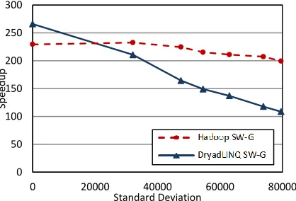
Figure 9 presents the execution time taken for the ran-domly distributed inhomogeneous data sets with the same mean length, by the two different implementations, while figure 10 presents the executing time taken for the skewed distributed inhomogeneous data sets. The Dryad results depict the Dryad performance adjusted for the performance difference of the NAligner and JAligner ker-nel programs. As we notice from the figure 9, both im-plementations perform satisfactorily for the randomly distributed inhomogeneous data, without showing signif-icant performance degradations with the increase of the standard deviation. This behavior can be attributed to the fact that the sequences with varying lengths are randomly distributed across a data set, effectively providing a natu-ral load balancing to the execution times of the sequence blocks.

Fig. 10. Performances of SW-G pairwise distance calculation appli-cation for skewed distributed inhomogeneous data with „400‟ mean sequence length.

For the skewed distributed inhomogeneous data, we notice clear performance degradation in the Dryad im-plementation. Once again the Hadoop implementation performs consistently without showing significant per-formance degradation, even though it does not perform as well as its randomly distributed counterpart. The Ha-doop implementations’ consistent performance can be attributed to the global pipeline scheduling of the map tasks. In the Hadoop Smith-Waterman implementation, each block gets assigned to a single map task. Hadoop framework allows the administrator to specify the num-ber of map tasks that can be run on a particular compute node. The Hadoop global scheduler schedules the map tasks directly on to those placeholders in a much finer granularity than in Dryad, as and when the individual map tasks finish. This allows the Hadoop implementation to perform natural global load balancing. In this case it might even be advantageous to have varying task execu-tion times to iron out the effect of any trailing map tasks towards the end of the computation. Dryad implementa-tion pre allocates all the tasks to the compute nodes and does not perform any dynamic scheduling across the

0 1,000 2,000 3,000 4,000 5,000 6,000

0 50 100 150 200 250 300

To

tal

T

im

e (

s)

Standard Deviation

DryadLINQ SW-G

Hadoop SW-G

1000 1100 1200 1300 1400 1500 1600 1700 1800

0 50 100 150 200 250 300

Tim

e

(s)

Standard Deviation

Hadoop SW-G

nodes. This makes a node which gets a larger work chunk to take considerable longer time than a node which gets a smaller work chunk, making the node with a smaller work chuck to idle while the other nodes finish.

4.2.2 CAP3

Unlike in Smith-Waterman Gotoh (SW-G) implementa-tions, CAP3 program execution time does not directly depend on the file size or the size of the sequences, as it depend mainly on the content of the sequences. This made it hard for us to artificially generate inhomogene-ous data sets for the CAP3 program, forcing us to use real data. When generating the data sets, first we calculated the standalone CAP3 execution time for each of the files in our data set. Then based on those timings, we created data sets that have approximately similar mean times while the standard deviation of the standalone running times is different in each data set. We performed the per-formance testing for randomly distributed as well as skewed distributed (sorted according to individual file running time) data sets similar to the SWG inhomogene-ous study. The speedup is taken by dividing the sum of sequential running times of the files in the data set by the parallel implementation running time.

Fig. 11. Performance of Cap3 application for random distributed inhomogeneous data.

Fig. 12. Performance of Cap3 Applications for skewed distributed inhomogeneous data

Figures 11 & 12 depict the CAP3 inhomogeneous perfor-mance results for Hadoop & Dryad implementations.

Hadoop implementation shows satisfactory scaling for both randomly distributed as well as skewed distributed data sets, while the Dryad implementation shows satis-factory scaling in the randomly distributed data set. Once again we notice that the Dryad implementation does not perform well for the skewed distributed inhomogeneous data due to its static non-global scheduling.

4.2.3 Discussion on Inhomogeneity

Many real world data sets and problems are inhomoge-neous in nature making it difficult to divide those compu-tations into equally balanced computational parts. But at the same time most of the inhomogeneity of problems are randomly distributed providing a natural load balancing inside the sub tasks of a computation. We observed that the scheduling mechanism employed by both Hadoop (dynamic) and DryadLINQ (static) perform well when randomly distributed inhomogeneous data is used. Also in the above study, we observed that given there are suf-ficient map tasks, the global queue based dynamic sched-uling strategy adopted by Hadoop provide load balanc-ing even in extreme scenarios like skewed distributed inhomogeneous data sets. The static partition based scheduling strategy of DryadLINQ does not have the abil-ity to load balance such extreme scenarios. It is possible, however, for the application developers to randomize such data sets before using them with DryadLINQ, which will allow such applications to achieve the natural load balancing of randomly distributed inhomogeneous data sets we described above.

4.3 Performance in the Cloud

With the popularity of the computing clouds, we can no-tice the data processing frameworks like Hadoop, Map Reduce and DryadLINQ are becoming popular as cloud parallel frameworks. We measured the performance and virtualization overhead of several MPI applications on the virtual environments in an earlier study [24]. Here we present extended performance results of using Apache Hadoop implementations of SW-G and Cap3 in a cloud environment by comparing Hadoop on Linux with Ha-doop on Linux on Xen [26] para-virtualised environment. While the Youseff, Wolski, et al. [27] suggests that the VM’s impose very little overheads on MPI application, our previous study indicated that the VM overheads de-pend mainly on the communications patterns of the ap-plications. Specifically the set of applications that is sensi-tive to latencies (lower communication to computation ration, large number of smaller messages) experienced higher overheads in virtual environments. Walker [28] presents benchmark results of the HPC application per-formance on Amazon EC2, compared with a similar bare metal local cluster, where he noticed 40% to 1000% per-formance degradations on EC2. But since one cannot have complete control and knowledge over EC2 infrastructure, there exists too many unknowns to directly compare the-se results with the above mentioned results.

0 50 100 150 200 250 300

0 20000 40000 60000 80000

Sp

ee

d

u

p

Standard Deviation

DryadLinq Cap3

Hadoop Cap3

0 50 100 150 200 250 300

0 20000 40000 60000 80000

Spe

ed

u

p

Standard Deviation

DryadLinq Cap3

4.3.1 SW-G Pairwise Distance Calculation

Figure 13 presents the virtualization overhead of the Ha-doop SW-G application comparing the performance of the application on Linux on bare metal and on Linux on Xen virtual machines. The data sets used is the same 10000 real sequence replicated data set used for the scala-bility study in the section 4.1.1. The number of blocks is kept constant across the test, resulting in larger blocks for larger data sets. According to the results, the performance degradation for the Hadoop SWG application on virtual environment ranges from 25% to 15%. We can notice the performance degradation gets reduced with the increase of the problem size.

Fig. 13. Virtualization overhead of Hadoop SW-G on Xen virtual machines.

Fig. 14. Virtualization overhead of Hadoop Cap3 on Xen virtual ma-chines.

In the xen para-virtualization architecture, each guest OS (running in domU) perform their I/O transfers through Xen (dom0). This process adds startup costs to I/O as it involves startup overheads such as communication with dom0 and scheduling of I/O operations in dom0. Xen architecture uses shared memory buffers to transfer data between domU’s and dom0, thus reducing the operation-al overheads when performing the actuoperation-al I/O. We can notice the same behavior in the Xen memory manage-ment, where page table operations needs to go through Xen, while simple memory accesses can be performed by the guest Oss without Xen involvement. According to the

above points, we can notice that doing few coarser grained I/O and memory operations would incur rela-tively low overheads than doing the same work using many finer grained operations. We can conclude this as the possible reason behind the decrease of performance degradation with the increase of data size, as large data sizes increase the granularity of the computational blocks.

4.3.2 CAP3

Figure 14 presents the virtualization overhead of the Ha-doop CAP3 application. We used the same scalability data set we used in section 4.1.2 for this analysis too. The performance degradation in this application remains con-stant - near 20% for all the data sets. CAP3 application does not show the decrease of VM overhead with the in-crease of problem size as we noticed in the SWG applica-tion. Unlike in SWG, the I/O and memory behavior of the CAP3 program does not change based on the data set size, as irrespective of the data set size the granularity of the processing (single file) remains same. Hence the VM overheads do not get changed even with the increase of workload.

4.3.3 Fluctuations in Results

Table 1 Systematic error of SWG and Cap3 applications

Appli-cation

Runtime Average

Time (s)

Standard Error

Error Per-centage

SWG Dryad

LINQ

2479.782 +/- 3.183 0.13%

Hadoop Bare Metal

1608.416 +/- 0.734 0.05%

Hadoop VM

1890.594 +/- 0.652 0.03%

CAP3 Dryad

LINQ

365.715 +/- 5.027 1.37%

Hadoop Bare Metal

421.91 +/- 0.411 0.10%

Hadoop VM

511.002 +/- 1.543 0.30%

Since many experiments performed to obtain the results presented in this paper are long running, we did not have the luxury of performing each experiment multiple times to calculate errors for each single experiment due to re-source and time limitations. In order to compensate for that, we ran a single representative experiment from each of the application 20 times to find the systematic errors and fluctuations of the applications, which are presented in table 1. According to table 1, we can notice the system-atic errors to be very minimal for the experiments we per-formed. For the SWG applications, we performed Pair-wise alignment on 15,000 sequences, resulting in approx-imately 114 million actual sequence alignments. For the Cap3 applications we performed Cap3 sequence assembly on 1024 Fasta files. It should be noted that the systematic timing errors due to minor system fluctuations do not

0.00 0.01 0.01 0.02 0.02 0.03

10000 20000 30000 40000 50000

0% 10% 20% 30% 40% 50% 60%

Ti

m

e

pe

r

A

ct

ua

l Cal

cul

at

io

n

(m

s)

No. of Sequences

P

er

fo

rm

an

ce

D

eg

rad

at

io

n

o

n

VM

Perf. Degradation On VM (Hadoop) Hadoop SWG on VM

Hadoop SWG on Bare Metal

0% 10% 20% 30% 40% 50% 60%

0.3 0.35 0.4 0.45 0.5 0.55

0 2000 4000 6000

VM

O

ve

rhe

ad

A

vg

. T

im

e

P

er

Fi

le

(

s)

No. of Files

have a significant effect on the overall running time of a single experiment due to the long running nature of the experiments. All the other experiment results presented in the paper are performed at least twice and the average time was taken.

5

C

P

M

The category of ―many-task computing‖ also belongs to the pleasingly parallel applications in which the parallel tasks in a computation perform minimum inter-task communications. From our perspective independent jobs or jobs with collection of almost independent tasks repre-sents the ―many-tasks‖ domain. Apart from the EST and pairwise distance computations we have described, ap-plications such as parametric sweeps, converting docu-ments to different formats and brute force searches in cryptography are all examples in this category of applica-tions. In this section we compare the programming styles of the three parallel runtimes that we have evaluated. The motivation behind this comparison is to show the reader the different styles of programming supported by the above runtimes and the programming models one needs to use with different runtimes. This is by no means an exhaustive study of programming techniques.

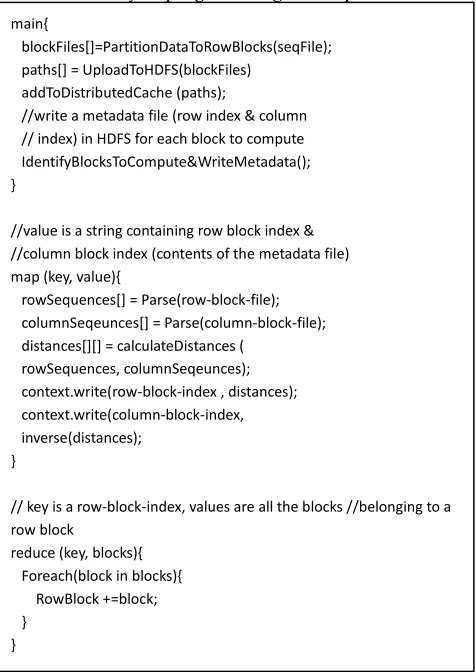
Fig. 15. Code segment showing the MapReduce implementation of pairwise distance calculation using Hadoop.

One can adopt a wide range of parallelization tech-niques to perform most of the many-task computations in

parallel. Thread libraries in multi-core CPUs, MPI, classic job schedulers in cloud/cluster/Grid systems, independ-ent ―maps‖ in MapReduce, and independindepend-ent ―vertices‖ in DryadLINQ are all such techniques. However, factors such as the granularity of the independent tasks, the amount of data/compute intensiveness of tasks deter-mine the applicability of these technologies to the prob-lem at hand. For example, in CAP3 each task performs highly compute intensive operation on a single input file and typically the input files are quite small in size (com-pared to highly data intensive applications), which makes all the aforementioned techniques applicable to CAP3. On the other hand the pairwise distance calculation applica-tion that requires a reducapplica-tion (or combine) operaapplica-tion can easily be implemented using MapReduce programming model.

To clarify the benefits of the cloud technologies, we will consider the following pseudo code segments repre-senting Hadoop, DryadLINQ and MPI implementations of the pairwise distance (Smith Waterman dissimilarities) calculation application (discussed in section 3.1.2).

In Hadoop implementation the map task calculates the Smith Waterman distances for a given block of sequences while the reduce task combine these blocks to produce row blocks of the final matrix. The MapReduce pro-gramming model executes map and reduce tasks in paral-lel (in two separate stages) and handles the intermediate data transfers between them without any user interven-tion. The input data, intermediate data, and output data are all stored and accessed from the Hadoop’s distributed file system (HDFS) making the entire application highly robust.

The DryadLINQ implementation resembles a more query style implementation in which the parallelism is completely abstracted by the LINQ operations, which are performed in parallel by the underlying Dryad runtime. The ―PerformAlignments‖ function has a similar capabil-ity to a map task and the ―PerformMerge‖ function has a similar capability to the reduce task in MapReduce. Dry-adLINQ produces a directed acyclic graph (DAG) for this program in which both ―SelectMany‖ and the ―Apply‖ operations are performed as a collection of parallel verti-ces (tasks). The DAG is then executed by the underlying Dryad runtime. DryadLINQ implementation uses Win-dows shared directories to read input data, store and transfer intermediate results, and store the final outputs. With replicated data partitions, DryadLINQ can also support fault tolerance for the computation.

Input parameters of the MPI application include a FASTA file, thread, process per node, and node count. In the data decomposition phase, subsets of sequences are identified as described in section 3.1.5. Corresponding to MPI runtime architecture in Figure 6(right), we use MPI.net [18] API to assign parallel tasks to processes (de-fault is one per core). One can use fewer processes per node and multi-threading in each MPI process (and this is most efficient way to implement parallelism for MDS and PWClustering) but we will not present these results here.

main,

blockFiles*+=PartitionDataToRowBlocks(seqFile); paths*+ = UploadToHDFS(blockFiles)

addToDistributedCache (paths);

//write a metadata file (row index & column // index) in HDFS for each block to compute IdentifyBlocksToCompute&WriteMetadata(); -

//value is a string containing row block index & //column block index (contents of the metadata file) map (key, value),

rowSequences*+ = Parse(row-block-file); columnSeqeunces*+ = Parse(column-block-file); distances*+*+ = calculateDistances (

rowSequences, columnSeqeunces); context.write(row-block-index , distances); context.write(column-block-index, inverse(distances);

-

// key is a row-block-index, values are all the blocks //belonging to a row block

reduce (key, blocks), Foreach(block in blocks), RowBlock +=block; -

Main(),

//Calculate the block assignments assignBlocksToTasks();

//Perform allignment calculation for each block //Group them according to their row numbers //Combine rows to form row blocks

outputInfo = assignedBlocks .SelectMany(block =>

PerformAlignments(block)) .GroupBy(x => x.RowIndex);

.Apply(group=>PerformMerge(group));

//Write all related meta data about row blocks and // the corresponding output files.

writeMetaData(); -

//Homomorphic property informs the compiler //that each block can be processed separately.

*Homomorphic+

PerformAlignments(block),

distances*+=calculateDistances(block); writeDistancesToFiles();

-

*Homomorphic+ PerformMerge(group),

mergeBlocksInTheGroup(group); writeOutputFile();

-

using (MPI.Environment env = new MPI.Environment(ref args)), sequences = parser.Parse(fastaFile);

size = MPI.Intracommunicator.world.Size; rank = MPI.Intracommunicator.world.Rank; partialDistanceMatrix*+*+*+ = new short

*size+*blockHeight+*blockWidth+;

//Compute the distances for the row block for (i =0; i< noOfMPIProcesses; i++), if (isComputeBlock(rank,i)), partialDistanceMatrix*i+ =

computeBlock(sequences, i,rank); -

-

MPI_Barrier();

// prepare the distance blocks to send

toSend*+ =transposeBlocks(partialDistanceMatrix);

//use scatter to send & receive distance blocks //that are computed & not-computed respectively

for (receivedRank = 0; receivedRank < size; receivedRank++),

receivedBlock*+*+ =

MPI_Scatter<T*+*+>(toSend, receivedRank); if (isMissingBlock(rank,receivedRank)), partialMatrix*receivedRank+ = receivedBlock; -

-

MPI_Barrier();

//Collect all distances to root process. if (rank == MPI_root),

partialMatrix.copyTo(fullMatrix); for(i=0;i<size;i++),

if (rank != MPI_root),

receivedPartMat=MPI_Receive<T*+*+>(i, 1); receivedPartMat.copyTo(fullMatrix); -

-

fullMatrix.saveToFile(); -else,

MPI_Send<t*+*+>(partialMatrix, MPI_root, 1); -

-

Each compute node has a copy of the input file and out-put results written directly to a local disk. In this MPI example, there is a Barrier call followed by the scatter communication at the end of computing each block. This is not the most efficient algorithm if the compute times per block are unequal but was adopted to synchronize the communication step.

The code segments (Figure 15 Hadoop MapReduce, figure 16 DryadLINQ, and figure 17 MPI) show clearly how the higher level parallel runtimes such as Hadoop and DryadLINQ have abstracted the parallel program-ming aspects from the users. Although the MPI algorithm we used for SW-G computation uses only one MPI com-munication construct (MPI_Scatter), in typical MPI appli-cations the programmer needs to explicitly use various communication constructs to build the MPI communica-tion patterns. The low level communicacommunica-tion contracts in MPI supports parallel algorithms with variety of commu-nication topologies. However, developing these applica-tions require great amount of programming skills as well.

Fig. 16. Code segment showing the DryadLINQ implementation of pairwise distance calculation.

On the other hand, high level runtimes provide limited communication topologies such as map-only or map

fol-lowed by reduce in MapReduce and DAG base execution flows in DryadLINQ making them easier to program. Added support for handling data and quality of services such as fault tolerance make them more favorable to de-velop parallel applications with simple communication topologies. Many-task computing is an ideal match for these parallel runtimes.

Fig. 17. Code segment showing the MPI implementation of pairwise distance calculation.

oriented towards memory to memory operations whereas Hadoop and DryadLINQ are file oriented. This difference makes these new technologies far more robust and flexi-ble. However, the file orientation implies that there is much greater overhead in the new technologies. This is a not a problem for initial stages of data analysis where file I/O is separated by a long processing phase. However as discussed in [12], this feature means that one cannot exe-cute efficiently on MapReduce and traditional MPI pro-grams that iteratively switch between ―map‖ and ―com-munication‖ activities. We have shown that an extended MapReduce programming model named Twister [19][7] can support both classic MPI and MapReduce operations. Twister has a larger overhead than good MPI implemen-tations but this overhead does decrease to zero as one runs larger and larger problems.

6

R

W

There have been several papers discussing data analysis using a variety of cloud and more traditional clus-ter/Grid technologies with the Chicago paper [20] influ-ential in posing the broad importance of this type of prob-lem. The Notre Dame all pairs system [21] clearly identi-fied the ―doubly data parallel‖ structure seen in all of our applications. We discuss in the Alu case the linking of an initial doubly data parallel to more traditional ―singly data parallel‖ MPI applications. BLAST is a well-known doubly data parallel problem and has been discussed in several papers [22][23]. The Swarm project [6] successful-ly uses traditional distributed clustering scheduling to address the EST and CAP3 problem. Note approaches like Condor can have significant startup time dominating performance. For basic operations [24], we find Hadoop and Dryad get similar performance on bioinformatics, particle physics and the well-known kernels. Wilde [25] has emphasized the value of scripting to control these (task parallel) problems and here DryadLINQ offers some capabilities that we exploited. We note that most previous work has used Linux based systems and technologies. Our work shows that Windows HPC server based sys-tems can also be very effective.

7

C

We have studied two data analysis problems with three different technologies. They have been looked on machines with up to 768 cores with results presented here run on 256 core clusters. The applications each start with a “doubly data-parallel” (all pairs) phase that can be implemented in MapReduce, MPI or using cloud resources on demand. The flexibility of clouds and MapReduce suggest they will be-come the preferred approaches. We showed how one can support an application (Alu) requiring a detailed output structure to allow follow-on iterative MPI computations. The applications differed in the heterogeneity of the initial data sets but in each case good performance is observed, with the new cloud MapReduce technologies competitive with MPI

performance. The simple structure of the data/compute flow and the minimum inter-task communicational requirements of these “pleasingly parallel” applications enabled them to be implemented using a wide variety of technologies. The support for handling large data sets, the concept of moving computation to data, and the better quality of services pro-vided by the cloud technologies, simplify the implementa-tion of some problems over tradiimplementa-tional systems. We find that different programming constructs available in MapReduce, such as independent “maps” in MapReduce, and “homo-morphic Apply” in DryadLINQ, are suitable for implement-ing applications of the type we examine. In the Alu case, we show that DryadLINQ and Hadoop can be programmed to prepare data for use in later parallel MPI/threaded applica-tions used for further analysis. We performed tests using identical hardware for Hadoop on Linux, Hadoop on Linux on Virtual Machines and DryadLINQ on HPCS on Win-dows. These show that DryadLINQ and Hadoop get similar performance and that virtual machines give overheads of around 20%. We also noted that support of inhomogeneous data is important and that Hadoop currently performs better than DryadLINQ unless one takes steps to load balance the data before the static scheduling used by DryadLINQ. We compare the ease of programming for MPI, DryadLINQ and Hadoop. The MapReduce cases offer higher level interface and the user needs less explicit control of the parallelism. The DryadLINQ framework offers significant support of database access but our examples do not exploit this.

A

The authors wish to thank our collaborators from Biology whose help was essential. In particular Alu work is with Haixu Tang and Mina Rho from Bioinformatics at Indiana University and the EST work is with Qunfeng Dong from Center for Genomics and Bioinformatics at Indiana Uni-versity. We appreciate all SALSA group members, espe-cially Dr. Geoffrey Fox, Scott Beason, and Stephen Tak-Lon Wu for their contributions. We would like to thank Microsoft for their collaboration and support. Tony Hey, Roger Barga, Dennis Gannon and Christophe Poulain played key roles in providing technical support.

R

[1] J. Dean, and S. Ghemawat, ―MapReduce: simplified data pro-cessing on large clusters,‖ Commun. ACM vol. 51, no. 1, pp. 107-113, 2008.

[2] M. Isard, M. Budiu, Y. Yu, A. Birrell, D. Fetterly, ―Dryad: Dis-tributed data-parallel programs from sequential building blocks,‖ European Conference on Computer Systems, March 2007. [3] Y.Yu, M. Isard, D. Fetterly, M. Budiu, Ú. Erlingsson, P. Gunda,

J. Currey, ―DryadLINQ: A System for General-Purpose Distrib-uted Data-Parallel Computing Using a High-Level Language,‖

Symposium on Operating System Design and Implementation (OSDI), 2008.