International Journal of Innovative Technology and Exploring Engineering (IJITEE) ISSN: 2278-3075,Volume-8, Issue-9S3, July 2019
Abstract: Noise removal from images is among the challenging processes for researches. Image denoising is a crucial step to improve 3D image conspicuity and to enhance the performance of all the processing needs of quantitative image analysis. Magnetic Resonance (MR) imaging has an increasing importance in the field of medical diagnosis. MR 3D image de-noising has two features (i) tri-dimensional structure of images and (ii) the nature of the noise, which are Rician & Gaussian. Kernel regression is one of 3D non-parametric noise level estimation technique which is effective than other denoising experimental filters. The proposed Fourth order Kernel Regression (FKR) algorithm builds an efficient and robust estimator and improves the accuracy of noise and it further improves the finer estimations of pixel value and its gradients. Experimental results demonstrate positively by achieving better performance, with respect to other de-noising filters.
KeyWords: Kernel regression, Median Filter, Medical Images, Rician Noise, Rican Median Absolute Deviation (RMAD) Estimator, Image denoising.
I. INTRODUCTION
Digitalized visual has come to be recognized as the means of communication in the present era. Images transmitted digitally are corrupted with noise, hence, have to be denoised before deploying them in applications [1],[ 3],[5].De-noising is done by manipulating the dataset of received image to produce high quality images. For removal of noise, knowledge about the level of noise and the type of noise is vital in selecting the appropriate de-noising algorithm. Magnetic Resonance Imaging is an imaging technique to diagnose medical conditions and the 3D images acquired are corrupted with noise and makes it difficult for interpretation [2],[4],[6]This practical difficulty is usually overcome by reducing the noise in the images. Usually Rician noise is incorporated in the MR images and they suffer from a contrast reducing signal dependent bias. The image used to be enhanced earlier by modifying the parameters of the MRI device, however, in these earlier methods, number of test images used for analyzing is more and hence time consuming.
Classical image processing parametric methods rely on a specific model while computing vital parameters. This process depends on diverse problems ranging from denoising,
Revised Manuscript Received on July 22, 2019.
B.Sundarraj, , Department of CSE, Bharath Institute of Higher Education and Research, Chennai, Tamilnadu, India.
S. Sri Gowtham, Department of CSE, Bharath Institute of Higher Education and Research, Chennai, Tamilnadu, India.
C.Nalini, Department of CSE, Bharath Institute of Higher Education and Research, Chennai, Tamilnadu, India.
up-scaling and interpolation. A generative model based upon the estimated parameters is then produced as the best estimate of the underlying signal. Kernel regression is deployed in order to ascertain the conditional expectation of the noiseless pixel value with respect to the pixel coordinates of another image. There are three types of regressions namely parametric,non-parametric and local polynomial regression.
Parametric regression can be derived as y = f(x) + e, where known smooth functions is represented as f. In non-parametric regression f represents unknown smooth function and is unspecified by regression of modular parametric [7],[9],[11]. Weighted Least Squares (WLS) is used by Local polynomial regression to fit dth degree (d≠0) to data. The weights assigned to the observations are determined by an “Initial Kernel Regression Fit” to the data. For image denoising and enhancement, a non-parametric estimation technique called kernel regression can be applied successfully.
II. BACKGROUNDWORK
Presence of Rician noise in MR intensity images is governed by Rician distribution. Rayleigh distribution function is used to generate Rician noise in images mathematically. The acquired, untreated image data is tainted by Additive White Gaussian Noise (AWGN), which is a complex value. The variance σ of the noise is taken as same for both the real and assumed complex values [9,10]. MR image is received as a magnitude of the complex values. The resulting pixels are therefore corrupted by Rician noise. Let ith pixel of given image in 3D coordinate represents xi ϵ [1,M] × [1,N] ×[1,P]. Assume ti is true value (noiseless) and qi is observed value
(noisy). The true values of pixel lie in [0, v] range and v = 255 (maximum pixel value).
Two component vectors
2 2
( (x )) ( (x ))
i i i
t
, is the magnitude of ti, where α and χ are real and imaginary values.
The equation of observed value is
2 2
( (x ) ) ( (x ) )
i i i i i
q
which has Rician noise. The square of the observed value [3, 15] is given by Equation 1
2 2 2
[
i]
[
i] 2
E q
E t
(1)To achieve best result in terms of robustness and accuracy, Rician Median Absolute Deviation (RMAD) estimator is applied primarily, to remove bias from squared magnitude image and subsequently
denoising the magnitude of MR image. For the images where no
3D MR Image Denoising using higher Order
Kernel Regression
background is available, this estimator is proposed, subject to approximation of Gaussian noise within the object. The methods for RMAD Estimation are classified as methods using background areas for estimating noise variance and image object.
In RMAD estimator equation ti is given by Equation 2
2 2
max(0,
2
)
i i
t
q
(2)
Physically insignificant complex values can be evaded using maximum function
2 2
(x )
it
i2
z
(3)
2
i i
y
q
(4)
III. EXISTING KERNEL REGRESSION MODULES
Existing image denoising system consists of four modules. Once the Rician noise level is estimated, a pre-processing task helps to obtain original image’s gradients and its pilot estimation. Following this, better inference is ascertained by deploying the same method. Eventually, the kernel regression of second order helps to evaluate weights based on filter of zeroth order. This performance is comparable with Unbiased Kernel Regression Filter (UKR)
A. Rician Noise Estimation
To have reliable estimation of noise level without human intervention for MR images, this estimation is optimum. Assuming the noise variance to be the same in both the real and imaginary parts of the raw and complex MR data are believed to be corrupted by white additive Gaussian noise [8],[10] ,[12]A general two-step process is involved in noise estimation:
(i) Squaring the input image and (ii) Noise estimation.
In this module first, the bias from the squared magnitude image is removed using unbiased estimator and then denoising is applied to the magnitude of MR image.
Unbiased estimator: A statistical method used to estimate a population parameter is said to be unbiased, if the mean of a sampling distribution of statistical marker equals the true value of the estimated parameter.
B. Pre-Processing
The objective of the pre-processing module is to estimate the original image and its gradients in three spatial directions [25],[27],[29].As the simple median filter over a 3x3x3 generates reasonable results with limited effort, it has been chosen as the primary filter which is applied to the squared input values. The median filter values obtained as output is applied through a set of four convolution filters to obtain approximations of the original values and its gradients. Median Filtering: A non-linear digital filtering technique is often used to eradicate noise; such noise reduction is typically a preprocessing step used to enhance the results of the image denoising parameters (for example, edge detection on an
image). Median Filtering preserves edges while removing noise, is therefore deployed in digital image processing. [38],[40].
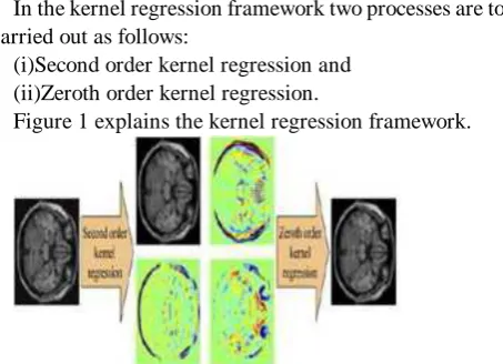
C. Kernel Regression Framework
In the kernel regression framework two processes are to be carried out as follows:
(i)Second order kernel regression and (ii)Zeroth order kernel regression.
[image:2.595.309.536.135.299.2]Figure 1 explains the kernel regression framework.
Figure 1. Kernel Regression Framework
Second Order Kernel Regression: This module serves to refine the tentative values of the original image and its gradients that occur at the pre-processing stage. Under kernel regression framework, the original biased values are estimated. The assessed values of original image, horizontal and vertical gradients are computed.
The performance is estimated to be superior, if Ki is the
preferred steering kernel.
Zeroth Order Kernel Regression: The zeroth order kernel regression computes the weighted average of pixels in a suitable neighborhood. The basis of the proposed method is obtained by the computation of weights for averaging from similar-feature vectors associated with each of the image pixels.
D. Bias Correction
Bias correction serves to derive the final estimation of the noiseless values, by correcting the Rician noise bias and reversal of the square of the pixel values. To measure the denoising performance, four quantitative measures are used as follows,
(i) Peak Signal to Noise Ratio (PSNR), (ii) Mean squared Error (MSE) and (iii) Structural Similarity Index (SSIM).
Unbiased estimator: A computation serves to arrive at an equitable population parameter wherein the mean of the sampling distribution equals the real value of the estimated parameter. A statistic d is called an unbiased estimator for a function of the parameter g(θ) provided that for every choice of θ,
( )
( )
E d X
g
(5) An estimator in simple word called as biased if the same is unbiased and the difference can beInternational Journal of Innovative Technology and Exploring Engineering (IJITEE) ISSN: 2278-3075,Volume-8, Issue-9S3, July 2019
( )
( )
( )
d
b
E d X
g
(6) Quality of Estimator: Mean Square error is computed to estimate the Quality of estimator.2 2
[( ( ) ( )) ] [ ( ) ( ) d( ) ]
E d X g E d X E d X b (7)
2 2
[( ( )
( )) ] 2 ( )( [ ( )
d( )]
d( ) ]
E d X
E d X
b
E d X
E d X
b
(8)
2
( ( ))
d( )
Var d X
b
(9) Existing Second Order Kernel Regression models produce fairly reasonable estimation for further processing, nonetheless, the original noisy data cannot be ignored or discarded, as valuable information from noiseless images is lost in subsequent filtering process.The proposed Fourth Order Kernel Regression performs better than the existing, innovative denoising techniques in terms of handing Rician noise at higher levels and in obtaining well-defined, denoised images with fewer artifacts.
IV. PROPOSED FOURTH ORDER KERNEL REGRESSION MODEL
Preliminary estimation of the original image and its three spatial direction gradients are obtained by using steering kernel regression. In order to produce such approximation with minimal calculations, pre-processing module is emphasized. As mentioned in [26],[28],[30], simple median filter over a 3x3x3 window is applied to yield reasonable results in less effort. It is applied to squared input of yi to obtain median filtered values ˜yi. Outcome of this filter is supplemented to a set of diffusion filter for extracting estimations of original value and its gradients, as stated below[13], [15] ,[17]
Gaussian low pass filter is considered as the first intricacy filter having smoothing parameter δ
2 2 2 1 2 3
0 0 1 2 3 3 2
3 2
x x x
1
(x) (x , x , x ) exp( )
f f
(10)For obtaining an approximation of true biased image z as :
0
ˆ
*
z
y
f
y
%
(11)
Where median of filtered imaged is denoted as ˜yi and convolution operator is denoted as *.
This process tends to extend the corresponding smoothed estimators to spatial directions.
ˆ
ˆ
*
j j jz
y
f
y
x
x
(12)Using 3D Discrete Fourier Transform (DFT), convolutions in Equations 11 and 12 are computed to speed up the process. Further to the frame work of Kernel Regression, the original biased value z(xi) is estimated as yi based on the observation of mean regression function [11].
( )
( )
[ ]
i i i i i
y
z x
e
z x
E y
(13)
where
e
iis the error term for ith pixel and E[e
i] = 0. FromEquations 3, 5 and 6, the image arbitrary position is x, and its components are not integers, where x is represented by
1
( )
...
2
i i i i
T T
x
x
x
x
x
x
z
z
z
x
H
z x
x
x
(14)
where
z
is Gradient Operator andH
z
is Hessian Operator, while Hessian Matrix considered as symmetric, it simplifies to
0 1
2
} ...T
T T
i i i
T
i
x x x vech x x x x
z
(15)
where vech is a vectorization of 3x3 symmetric matrix.
a
b
c
vech
b
d
e
c
e
f
= (a b c d e f)T(16) Then, by comparing Equations 14 and 15, it is suggested, pixel value of interest β0 = z(x) and vector β0 and β1 are :
1
1 2 3
( )
( )
( )
( )
,
,
T
z x
z x
z x
z x
x
x
x
(17)2 2 2 2 2 2
2 2 2 2
1 1 2 1 3 2 2 3 3
( ) ( ) ( ) ( ) ( ) ( )
, 2 , 2 , , 2 ,
T
z x z x z x z x z x z x
x x x x x x x x x
(18) 0
[
,...,
TN]
b
(19)
where N is the order of approximation and in this case N = 4. The value of β0 (the estimated value of the original image at
x) and β1 (the estimated value of the 3D gradient at x) are the
interested values.
Optimization problem of Vector b parameter can be resolved as following:
arg min
( )
b
b
$
F b
0 1
2 2
( )
( ) (x
)(
(x
)
((x
)(x
) ) ...) .
T
i i i i i i
i
T T
i i
F b
k y K
x y
x
vech
x
x
(20)where Ki is the 3D smoothing kernel function for pixel i and ki. An additional kernel is introduced for giving more prominence to those pixels i, whose observed value yi is likely more close to original value z(x). It is computed as follows:
2
(
)
1
i ii
y
y
k
%
(21)where it is to be remembered that, ˜yi is already computed media filtered value and ki(yi) ϵ
Kernel
k
i is introduced into the function to minimize the same in Equation 20. This helps to reduce those pixels’ influence which depart largely from median of its 3x3x3 window and are experienced with high noise corruption. Below equation in matrix form can be optimized by rewriting as:2
arg min arg min( ) ( )
X
T
X W X X X
b b
b$ yX b yX b W yX b
Where
1 2 0 1
[ ,
,...,
P] ,
T[
,
T,...,
TN]
Ty
y y
y
b
1( )
1 1(x
1),...,
(
)
(x
)
X P P P P
W
diag k y K
x
k
y K
x
1 1 1
2 2 2
1
(x
)
{(x
)(x
) }
1 (x
)
{(x
)(x
) }
1 (x
)
{(x
)(x
) }
T T T
T T T
X
T T T
P P P
x
vech
x
x
x
vech
x
x
X
x
vech
x
x
K
K
M
M
M
M
K
(22)
Wherein diag being a diagonal matrix produced by neighborhood position x. The number of pixels being P, for computing an estimate of image pixel value, without considering (N), the estimator order. In order to estimate the parameter of β0, the computations are limited and the simplified version of least-squares estimation will be:
1
0
e (X
1)
T T T
X X X X X
z
W X
X
W y
$
(23)
Wherein, the first element of column vector e1 equals to one and rest to Zero. While computing β0 for the N = 0 using N > 0 as estimator of high-order, fundamental difference exists. Effectively except β0 , discarding all estimated βns , estimates of pixel values are computed based on assumption that local polynomial structure of Nth is present.
1
(X
XT X X)
XT Xb
$
W X
X
W y
(24)
That the same is applicable, whenever
T
X X
X
W y
is invertible.
Subsequently, the smoothing kernel function Ki in Equation 20 is chosen and as seen in [13], the Kernel regression performance estimation is greatly enhanced. If Ki considered as a steering kernel, that is Ki depends on covariance matrix
Ci:
)
3 2
3 2
det(C
1
(x
x)
exp(
(x
x)
(x
x))
2
(2 )
i T
i i i i i
K
C
(25)wherein global smoothing parameter is ρ and is assumed that these energies and directions correspond to eigen decomposition of symmetric matrix Ci.
Ci proposed estimator reads as:
1
(
)
(y )
T
i i i i
i i
C
V S
I V
k
(26)
Where, Si is a 3x3 matrix of diagonal in nature, which is
representing dominant directions of the energy.
Vi represents 3x3 matrix of orthogonal in nature. The column
of this matrix represents its directions. λ represents regularization parameter of minor value, which, guarantees that Ci is non-singular even if Si has a zero element in its
diagonal. In addition to this, kernel ki(yi) helps in reducing
the influence of highly corrupted pixels.
Equation 20 and 25 inferring pixel i influence on values of its neighborhood pixels till it reaches further, as det Ci
diminishes and vice versa. The steering kernel Ki(xi−x)
depends on spatial separation (xi−x) and the pixel values of
yi, By using Ki instead of K is emphasized in this
mathematical notation.
The output is obtained based on the Original data weighted average using zeroth order Kernel Regression:
ˆz(x )
i
ijy
j(27)
By reversing the square of pixel values, the Rician noise bias has to be corrected, in order to yield final estimations for ti of
noiseless values.
2
ˆ
ˆ
t
i
max(0, z(x ) 2
i
(28)
Where σ is estimated in Equation 6.2 and have taken q2 2
ˆ(x )
i i
q
z
(29)
The proposed method has four modules namely : (i) Estimation of Rician noise level,
(ii) By preprocessing the original image gradients pilot estimation of the same is obtained.
(iii) Finer estimation is obtained using second and fourth order
steering kernel regression, and
(iv) Second order Kernel Regression is used for computing weights of zeroth order kernel regression output.
International Journal of Innovative Technology and Exploring Engineering (IJITEE) ISSN: 2278-3075,Volume-8, Issue-9S3, July 2019
[image:5.595.96.245.52.216.2]Figure 2. Fourth Order Kernel Regression model
Median Filtering: Digitally nonlinear technique of filtering is called median filter [14,15] and is generally deployed for noise removal. This is viewed as a preprocessing step in order to improve the results of subsequent processing such as edge detection on an image. It is used latently in digital image processing for removing noise while its edges are preserved [14],[ 16], [18].
Diffusion Filtering: The Diffusion Filtering is a discerning technique of linear filter for improving image quality and preserving its edges [37],[39],[41]. Each pixel of the image is applied with diffusion coefficients to define the smoothing extent required. When compared with the Gaussian smoothing and Wiener local empirical filter, this is effective, as the sharpness and contrast of the image is not affected.
Bias Correction: In order to obtain final estimations of noiseless values, the denoising method needs to correct the Rician noise bias and squared image pixel values to be reversed. To measure the denoising performance three quantitative measures are used viz: i) Mean squared Error (MSE), ii) Structural Similarity Index (SSIM) and iii) Peak Signal to Noise Ratio (PSNR).
Choice of Bandwidth: For non-parametric regressing fitting, appropriate bandwidth selection (smoothing parameter) is an essential element [19],[21],[23]. This model identifies balance between variance and bias to acquire an appropriate or good fit. The mean squared error criterion minimization is achieved through this identification method and helps to select an appropriate bandwidth for a dataset given.
V. IMPLEMENTATION 0F FOURTH ORDER KERNEL REGRESSION LEARNING MODEL
Summary of Fourth Order Kernel Regression denoising algorithm is as follows
Algorithm 1 - Fourth Order Kernel Regression
Require: Order of approximation N Ensure: Fourth Order Output
Step 1:
[
0,...,
]
T N
b
Where N is the order of approximation, in this case
N=4 and values of
0(the estimated value of theoriginal image at x) and
1 (the estimatedvalue of the three dimensional gradient at x).
Step 2:
0 parameter estimation is limited to estimatororder
N of the image pixel value and estimation of least square is derived as
1
0
e (X
1)
T T T
X X X X X
z
W X
X
W y
$
Where first element of e1 (column vector) =1 and remaining elements equal to 0.
Step 3: The fourth order Kernel evaluation yields estimated values of original image and its gradients. The construction of fourth order Kernel is the linear combination of two second order Kernels with the bandwidth h1 and h2 such that c = h1/h2.The fourth order Kernel is defined as,
K4 * = -k4/c2
The proposed Architecture is pictorially represented in Figure 2.
Algorithm 2 :Rician Noise estimation
Require: Rician Noise Level r Ensure: ti
Step 1: Rician noise level r to be estimated.
Step 2: From the estimated r, values are set for tunable parameters in subsequent steps: r, d, q, k and h (automated system).
Step 3: Input image to be squared and do pre-processing using
median filtering. After applying to diffusion filter, sample data of the pixel values and gradients are obtained.
Step 4: Kernel Regression to fourth order is to be carried out for evaluating assessed yield values of original image
and its gradients subsequently this output is applied to
second order regression.
Step 5: Kernel regression to second order is applied to obtain finer readings of pixel values and gradients, b0 and b1.
Step 6: Obtained results from Step 5 is used to build feature vectors, and the same is used to perform zeroth order Kernel regression filtering.
Step 7: Final output ti is obtained by correcting the bias of zeroth order Kernel regression filtered image and the
VI.EXPERIMENTALRESULTANDANALYSIS
The experimental results are carried out by using existing hardware setup and image database. The results for existing and proposed methods are verified by using MR 3D images which consists of 181 slices on each image type such as, T1- weighted, T2-weighted and Pd-weighted images. Denoising the MR image, smooth regions are filtered by the fourth order scheme and edges filtered by a second order scheme. During denoising the MR image, smooth regions are filtered by the fourth order scheme and edges filtered by a second order scheme. Sample images are shown in Figure 3.
[image:6.595.313.537.50.303.2](a) Brain Web T1 (b) Brain Web T2 (c) Brain Web Pd
Figure 3. MRI Brain Image
Database: The Proposed new method has been experimented using Internet Brain Segmentation Repository (ISBR) database and gave promising results. Currently there are six MR brain data sets, which were provided by the Center for Morphometric Analysis at Massachusetts General Hospital. Most of them have T1-weighted MR images of healthy subjects. Two data sets have images of two different patients with brain tumors. There are three different directories in which data sets can be found organized into “img”, “seg” and “otl” directories, which contain the raw, segmented and outlined images, respectively. However not all data sets have the “seg” and/or “otl” directories. Raw images are 256x256 of 16-bit, but some of them have also these images scaled to 8-bit. Segmented images are “trinary” images (pixels are labeled as a Grey Matter or White Matter tissue or as other),
with the same dimensionality as the raw
images[31],[33],[35]. Outlined images are the outcome of semi- automated segmentation techniques executed and contain indicators that define certain structures in each scan image. They are defined in a 512x512 grid, because they were created using over sampled images to double size. Parameter settings for the pre-computed brain database are three levels of intensity, non uniformity and modalities and five levels (1,3,5,7 and 9) of noise. The voxel values of each image are magnitude in nature and rather complex, imaginary or real.
MRI T1-weighted: Within the body, the difference of spin lattice is considered as T1. Subsequently various tissue relaxation times are referred as T1 weighted. Gradient or spin echo sequences are used to acquire images of T1 weighted. Gray and white substances are differentiated by appreciable contrast as provided by T1-weighted brain scans.
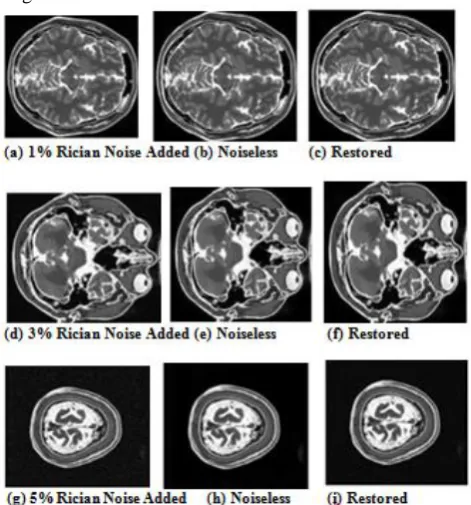
Figure 4. Results for Brain Web T1 weighted synthetic image
[image:6.595.46.262.208.288.2]MRI T2-weighted: Water is differentiated from fat as lighter and darker respectively as T2-weighted that is similar to weighted T1 scan.
Figure 5. Results for Brain Web T2 weighted synthetic image.
[image:6.595.308.544.369.622.2]International Journal of Innovative Technology and Exploring Engineering (IJITEE) ISSN: 2278-3075,Volume-8, Issue-9S3, July 2019
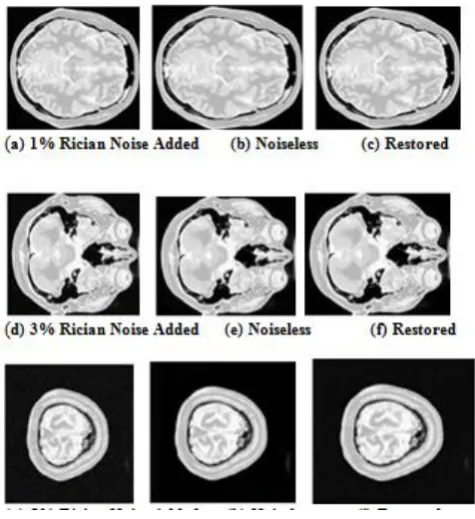
[image:7.595.304.549.51.198.2]
Figure 6. Results for Brain Web Pd weighted synthetic image.
Table 1 shows, that in the existing system maximum PSNR value achieved is 42.7172. In the proposed method, RMAD and diffusion filter play an important role in increasing higher PSNR (43.6481) for noise level (σ = 1) by preserving edges. RMAD plays another role in the reduction of MSE from 3.4782 to 2.8072 in the proposed method.
Table 1 : Performance Measures : Existing and proposed model T1 weighted image of Axial View
Table 2 shows for T2-weighted image, the PSNR value is low for noise level (σ = 1). Higher the noise level (above 1), the PSNR value is comparably higher than existing method.
Table : 2 Performance Measures for existing and proposed model for T2-weighted image of Axial View.
[image:7.595.50.288.54.314.2]In existing system, the maximum PSNR value is achieved 41.9949. In proposed method, RMAD and Diffusion Filter plays an important role to increase high PSNR (42.2917) for noise level (σ = 1) by preserving edges. RMAD play another role to reduce the MSE from 4.8296 to 4.1076 in the proposed method as shown in Table 3. Resulted images for T1 weighted MRI (Brain Web) are shown in Figure 4.
Table : 3 Performance Measures for existing and proposed model for Pd-weighted image of Axial View
Test
image/Method Noise added (in dB)
MSE RMSE PSNR SSIM
Proposed 1 4.1076 2.0267 42.2917 0.9860 Existing 4.8296 2.1976 41.9949 0.9833 Proposed 3 15.8563 3.9820 36.1288 0.9373 Existing 35.4161 5.9511 32.6388 0.8849 Proposed 5 28.7566 5.3625 33.5434 0.8983 Existing 91.6619 9.574 28.5089 0.7554 Proposed 7 42.6341 6.5295 31.8332 0.8546 Existing 146.0120 12.0835 26.4869 0.6867 Proposed 9 68.0639 8.2501 29.8016 0.8007 Existing 337.8333 18.3802 22.8438 0.5004
[image:7.595.301.553.318.459.2]Figure 7 shows the comparison result (RMSE) of the existing second order kernel regression and the proposed fourth order kernel regression for T1, T2, Pd weighted images. It clearly shows that RMSE of the proposed method is lesser than the existing method. Resulted images for T2 and Pd weighted MRI (Brain Web) are shown as Figure 5 and 6 respectively.
Figure 7. Comparison of RMSE value between Proposed and Existing method for T1,T2 and Pd Weighted images
Figure 8 shows the comparison result (PSNR) of the existing second order kernel regression and the proposed fourth order kernel regression for T1, T2, Pd weighted images. The value for PSNR is
[image:7.595.305.548.554.684.2]Figure 8. Comparison of PSNR value between Proposed and Existing method for T1,T2 and Pd Weighted images methods
[image:8.595.48.282.227.350.2]Figure 9. Comparison of SSIM value between Proposed and Existing method for T1,T2 and Pd Weighted images
[image:8.595.310.544.323.451.2]Figure 9 shows the comparison result (SSIM) of the existing second order kernel regression and proposed fourth order kernel regression for T1, T2, Pd weighted images. It clearly shows that the SSIM of the proposed method is greater than the existing method.
Figure 10. Comparison of Processing Time
Table 4 shows that the processing time of second order Kernel regression for T1- weighted image is increased when the noise level increase. For lower noise level, the processing time is minimal. Considering an example, when the moderate noise level is 3db, the processing time is 255.81 sec, whereas in proposed method by combining two second order Kernel with the bandwidth h1 and h2 linearly so we can achieve the processing time is 116.50 seconds for noise level 3dB.
Table : 4 Quantitative results for Brain Web T1-weighted image to calculate processing time (in seconds) for second order and fourth order Kernel regression.
Table 5 shows that the processing time of second order Kernel regression for T2- weighted image is increased when noise level increases. For lower noise level, the processing time is minimal. In fourth order Kernel regression for noise level (σ = 1, 3, 5, 7 and 9) the processing time increases gradually. For noise level above 9dB the processing time increases.
[image:8.595.50.282.463.587.2]Table: 5 Quantitative results for Brain Web T2-weighted image to calculate processing time (in seconds) for second order and fourth order Kernel regression
Table 6 shows the processing time of an existing method for Pd-weighted image varying non-linearly when noise level increases. In the proposed method the processing time is minimal as compared and varies slightly for different noise level.
Table :6 Quantitative results for Brain Web Pd-weighted image to calculate processing time (in seconds) for second order and fourth order Kernel regression
While estimating the Rician noise, Standard deviation from a 2D MRI image gets corrupted on the basis of the unevenness of the distribution. This method is not dependent on the background for noise estimation,
[image:8.595.309.547.591.708.2]International Journal of Innovative Technology and Exploring Engineering (IJITEE) ISSN: 2278-3075,Volume-8, Issue-9S3, July 2019
To estimate the sigma value, smoothing parameters are fixed in the preprocessing filter by reducing the constant value from 2000 to 1000.
Obtained sigma values are categorized into five ranges i.e., (i) Less than 0.021, (ii) Between 0.021 to 0.041, (iii)Between 0.041 to 0.067, (iv)Between 0.067 to 0.089 and (v) Greater than 0.089.
Depending on the ranges of sigma value, diffusion filter smoothing parameter, h, λ and local smoothing parameters are fixed. For sigma value less than 0.021- diffusion filter Smoothing parameter = 3.79597, h =0.98827, λ = 1.63609 and Local Smoothing parameter value = 0.000287814 are [20],[ 22], [24]
For obtained sigma value ranging between 0.021 to 0.041 the values are fixed as Diffusion Smoothing parameter = 3.90586, h=0.60711, λ = 0.110266 and Local Smoothing = 0.00077781.
For obtained sigma value ranging between 0.041 to 0.067 the values are fixed as Diffusion Smoothing parameter =5.17508, h=0.79454, λ = 0.13355 and Local smoothing parameter value = 0.0013252[32],[34],[36]
For obtained sigma value ranging between 0.067 to 0.089 the values are fixed as, diffusion Smoothing parameter = 4.54708, h=1.07039, λ = 0.3008 and Local smoothing parameter value =0.0021564.
For obtained sigma value greater than 0.089 the values are fixed as diffusion Smoothing parameter =4.8871, h=0.7803, λ =0.0209 and Local smoothing parameter value =0.0030891.
Image searching window size of 9x9x9 is replaced with 7x7x7 for all above ranges of sigma value. As the image window size is reduced the processing time using proposed algorithm reduces considerably.
VII. CONCLUSION
The proposed Fourth Order Kernel regression model yields an increase in PSNR value for the image; within computational time could produce enhanced quality images. This Kernel regression takes into consideration the combination of median and diffusion filter which improves the finer estimations of pixel value and its gradients. Viewed as an ill-posed problem, the proposed algorithm works to achieve satisfactory performance in general. Notwithstanding, this paves the way for further research work, which could bring about the use of next generation hybrid optimization-based denoising algorithms.
R
EFERENCES[1] Kumarave A., Rangarajan K.,Algorithm for automaton specification for exploring dynamic labyrinths,Indian Journal of Science and Technology,V-6,I-SUPPL5,PP-4554-4559,Y-2013
[2] P. Kavitha, S. Prabakaran “A Novel Hybrid Segmentation Method with Particle Swarm Optimization and Fuzzy C-Mean Based On Partitioning the Image for Detecting Lung Cancer” International Journal of Engineering and Advanced Technology (IJEAT) ISSN: 2249-8958, Volume-8 Issue-5, June 2019
[3] Kumaravel A., Meetei O.N.,An application of non-uniform cellular automata for efficient cryptography,2013 IEEE Conference on
Information and Communication Technologies, ICT 2013,V-,I-,PP-1200-1205,Y-2013
[4] Kumarave A., Rangarajan K.,Routing alogrithm over semi-regular tessellations,2013 IEEE Conference on Information and Communication Technologies, ICT 2013,V-,I-,PP-1180-1184,Y-2013 [5] P. Kavitha, S. Prabakaran “Designing a Feature Vector for Statistical
Texture Analysis of Brain Tumor” International Journal of Engineering and Advanced Technology (IJEAT) ISSN: 2249-8958, Volume-8 Issue-5, June 2019
[6] Dutta P., Kumaravel A.,A novel approach to trust based identification of leaders in social networks,Indian Journal of Science and Technology,V-9,I-10,PP--,Y-2016
[7] Kumaravel A., Dutta P.,Application of Pca for context selection for collaborative filtering,Middle - East Journal of Scientific Research,V-20,I-1,PP-88-93,Y-2014
[8] Kumaravel A., Rangarajan K.,Constructing an automaton for exploring dynamic labyrinths,2012 International Conference on Radar, Communication and Computing, ICRCC 2012,V-,I-,PP-161-165,Y-2012
[9] P. Kavitha, S. Prabakaran “Adaptive Bilateral Filter for Multi-Resolution in Brain Tumor Recognition” International Journal of Innovative Technology and Exploring Engineering (IJITEE) ISSN: 2278-3075, Volume-8 Issue-8 June, 2019
[10] Kumaravel A.,Comparison of two multi-classification approaches for detecting network attacks,World Applied Sciences Journal,V-27,I-11,PP-1461-1465,Y-2013
[11] Tariq J., Kumaravel A.,Construction of cellular automata over hexagonal and triangular tessellations for path planning of multi-robots,2016 IEEE International Conference on Computational Intelligence and Computing Research, ICCIC 2016,V-,I-,PP--,Y-2017 [12] Sudha M., Kumaravel A.,Analysis and measurement of wave guides
using poisson method,Indonesian Journal of Electrical Engineering and Computer Science,V-8,I-2,PP-546-548,Y-2017
[13] Ayyappan G., Nalini C., Kumaravel A.,Various approaches of knowledge transfer in academic social network,International Journal of Engineering and Technology,V-,I-,PP-2791-2794,Y-2017
[14] Kaliyamurthie, K.P., Sivaraman, K., Ramesh, S. Imposing patient data privacy in wireless medical sensor networks through homomorphic cryptosystems 2016, Journal of Chemical and Pharmaceutical Sciences92.
[15] Kaliyamurthie, K.P., Balasubramanian, P.C. An approach to multi secure to historical malformed documents using integer ripple transfiguration 2016 Journal of Chemical and Pharmaceutical Sciences92.
[16] A.Sangeetha,C.Nalini,”Semantic Ranking based on keywords extractions in the web”, International Journal of Engineering & Technology, 7 (2.6) (2018) 290-292
[17] S.V.GayathiriDevi,C.Nalini,N.Kumar,”An efficient software verification using multi-layered software verification tool “International Journal of Engineering & Technology, 7(2.21)2018 454-457 [18] C.Nalini,ShwtambariKharabe,”A Comparative Study On Different
Techniques Used For Finger – Vein Authentication”, International Journal Of Pure And Applied Mathematics, Volume 116 No. 8 2017, 327-333, Issn: 1314-3395
[19] M.S. Vivekanandan and Dr. C. Rajabhushanam, “Enabling Privacy Protection and Content Assurance in Geo-Social Networks”, International Journal of Innovative Research in Management, Engineering and Technology, Vol 3, Issue 4, pp. 49-55, April 2018. [20] Dr. C. Rajabhushanam, V. Karthik, and G. Vivek, “Elasticity in Cloud
Computing”, International Journal of Innovative Research in Management, Engineering and Technology, Vol 3, Issue 4, pp. 104-111, April 2018.
[21] K. Rangaswamy and Dr. C. Rajabhushanamc, “CCN-Based Congestion Control Mechanism In Dynamic Networks”, International Journal of Innovative Research in Management, Engineering and Technology, Vol 3, Issue 4, pp. 117-119, April 2018.
[22] Kavitha, R., Nedunchelian, R., “Domain-specific Search engine optimization using healthcare ontology and a neural network backpropagation approach”, 2017, Research Journal of Biotechnology, Special Issue 2:157-166
[23] Kavitha, G., Kavitha, R., “An analysis to improve throughput of high-power hubs in mobile ad hoc network” , 2016, Journal of Chemical and Pharmaceutical Sciences, Vol-9, Issue-2: 361-363
[24] Kavitha, G., Kavitha, R., “Dipping interference to supplement throughput in MANET” , 2016, Journal of Chemical and Pharmaceutical Sciences, Vol-9, Issue-2: 357-360
[25] Michael, G., Chandrasekar, A.,”Leader election based malicious detection and response system in
Sciences(JCPS) Volume 9 Issue 2, April - June 2016 .
[26] Michael, G., Chandrasekar, A.,”Modeling of detection of camouflaging worm using epidemic dynamic model and power spectral density”, Journal of Chemical and Pharmaceutical Sciences(JCPS) Volume 9 Issue 2, April - June 2016 .
[27] Pothumani, S., Sriram, M., Sridhar, J., Arul Selvan, G., Secure mobile agents communication on intranet,Journal of Chemical and Pharmaceutical Sciences, volume 9, Issue 3, Pg No S32-S35, 2016 [28] Pothumani, S., Sriram, M., Sridhar , Various schemes for database
encryption-a survey, Journal of Chemical and Pharmaceutical Sciences, volume 9, Issue 3, Pg NoS103-S106, 2016
[29] Pothumani, S., Sriram, M., Sridhar, A novel economic framework for cloud and grid computing, Journal of Chemical and Pharmaceutical Sciences, volume 9, Issue 3, Pg No S29-S31, 2016
[30] Priya, N., Sridhar, J., Sriram, M. “Ecommerce Transaction Security Challenges and Prevention Methods- New Approach” 2016 ,Journal of Chemical and Pharmaceutical Sciences, JCPS Volume 9 Issue 3.page no:S66-S68 .
[31] Priya, N.,Sridhar,J.,Sriram, M.“Vehicular cloud computing security issues and solutions” Journal of Chemical and Pharmaceutical Sciences(JCPS) Volume 9 Issue 2, April - June 2016
.
[32] Priya, N., Sridhar, J., Sriram, M. “Mobile large data storage security in cloud computing environment-a new approach” JCPS Volume 9 Issue 2. April - June 2016
[33] Anuradha.C, Khanna.V, “Improving network performance and security in WSN using decentralized hypothesis testing “Journal of Chemical and Pharmaceutical Sciences(JCPS) Volume 9 Issue 2, April - June 2016 . [34] Anuradha.C, Khanna.V, “A novel gsm based control for e-devices“
Journal of Chemical and Pharmaceutical Sciences(JCPS) Volume 9 Issue 2, April - June 2016 .
[35] Anuradha.C, Khanna.V, “Secured privacy preserving sharing and data integration in mobile web environments “ Journal of Chemical and Pharmaceutical Sciences(JCPS) Volume 9 Issue 2, April - June 2016 . [36] Sundarraj, B., Kaliyamurthie, K.P. Social network analysis for decisive
the ultimate classification from the ensemble to boost accuracy rates 2016 International Journal of Pharmacy and Technology 8 [37] Sundarraj, B., Kaliyamurthie, K.P. A content-based spam filtering
approach victimisation artificial neural networks 2016 International Journal of Pharmacy and Technology83.
[38] Sundarraj, B., Kaliyamurthie, K.P. Remote sensing imaging for satellite image segmentation 2016 International Journal of Pharmacy and Technology8 3.
[39] Sivaraman, K., Senthil, M. Intuitive driver proxy control using artificial intelligence 2016 International Journal of Pharmacy and Technology84.
[40] Sivaraman, K., Kaliyamurthie, K.P. Cloud computing in mobile technology 2016 Journal of Chemical and Pharmaceutical Sciences92. [41] Sivaraman, K., Khanna, V. Implementation of an extension for browser to detect vulnerable elements on web pages and avoid click jacking2016 Journal of Chemical and Pharmaceutical Sciences92.
AUTHORS PROFILE
B.Sundarraj, Assistant Professor, Department of Computer Science & Engineering, Bharath Institute of Higher Education and Research, Chennai, India
S.Sri Gowthem, Assistant Professor, Department of Computer Science & Engineering, Bharath Institute of Higher Education and Research, Chennai, India