Implementing intersection calculations of the ray tracing algorithm with systolic arrays

Rochester Institute of Technology

RIT Scholar Works

Theses

Thesis/Dissertation Collections

1987

Implementing intersection calculations of the ray

tracing algorithm with systolic arrays

Andrea Stankus

Follow this and additional works at:

http://scholarworks.rit.edu/theses

This Thesis is brought to you for free and open access by the Thesis/Dissertation Collections at RIT Scholar Works. It has been accepted for inclusion

in Theses by an authorized administrator of RIT Scholar Works. For more information, please contact

[email protected]

.

Recommended Citation

Roch

ester

I

n s

t i t

u

t e

of

T

e

c h

n

c

l cq

v

School

of

Computer

Sc

ien

ce

a

nd

Tec

h

n o l o

q v

I

m

p l e

me

n

t

i

n

g

Int e ~ seLt ion

C

al c ulati o n s

o

f

th

E:.

R

elY

T

r ac: i r

lg

Al

g orit h

m

w

i th

S

y s t o l

i

c::

Ar

ra

y

s

b

y

Andr

ea

St

an

kus

M

a

y

13

,

1

9

8

7

A

t

ll

e s l

s

s

ub mitt

ed

t

o

Til

e

F

a

c ul

l y o

f

th

e

S

choe l

of

C

Onlp u t l?l-

S

c

iep

ce

a

n d

T

e c hno l o g

y

in

p

ar

t

ial

f

i l f i llmen t

of

t

h l::

r-eq

u

i

r

em

en

t

s

f

o r

the deq

r e

c

-

0"

Mast e

r

a

f

Sci

enc e

in Cc

mou't.er-

Sc

i

euc

e

Ap

proved

B

y:

_ _ _ _ _ _ _ __ n

m

~

-

_

hl

r

lli r:r

Dr"

.

Do

n c

.

l<:l L.

Kr

-eh er

(

:d

'C

~

ij

)

GL.lY

J

oh n

s

on

Title of The I mp 1ement_{i ng} Intersec:11 on Calcul ations

of the

Ray

Tracing

Algorithm with

S ystolie Ar r a_ys

I Andr e a S ta nku. ?> here_{b y g}rant per m :i. ssion to Wallace

Memorial

Library,

- r r"'T"r J j..-.- -.. j-u._4^ who1e o r in _pa rt.

commercial use or profit. of RIT.

An_y r e_pr odu ctio

to reproduce _my thesis in

ACKNOWLEDGEMENT

I want to express _my sincere thanks arid appreciation

to Professor Gerald Johnson for

taking

the time to review

and critique this paper as it was

being

developed. I also

want to thank my committee?

Guy

Johnson,

Andrew Kitchen

arid Don Kreher for

helping

to define the final form of

ABSTRACT

Ray

tracing

is one technique that has been used to

synthesize realistic images with a computer.

Unfortunately,

this

technqiue,

when implemented in

software, is slow and expensive. The? trend in

computer-graphics has been toward the use of special purpose

hardware,

to speed _up the calculations, and,

hence,

the

generation of the synthesized image. This paper describes

the design and the operation of a systolic based

architecture, tailored to speed _up the intersection

calculations, that must be performed as a part of the _ray

TABLE OF CONTENTS

INTRODUCTION

1,1 STATEMENT OF PROBLEM 1

1.2 LITERATURE REVIEW 5

1.3 RAY TRACING IMPLEMENTATION 11

IMPLEMENTING RAY TRACING WITH TECHNIQUES FROM

IMAGE PROCESSING 13

2.1 DETAILED DESCRIPTION OF THE OFERATION OF

RAY TRACING ALGORITHM 13

2.2 INTRODUCTION TO SYSTOLIC ARRAYS 17

2.3 APPLICATION OF SYSTOLIC ARRAYS TO RAY TRACING 22

2.3.1 RAY TRACING AS A HIDDEN SURFACE REMOVAL

TECHNIQUE 22

2.3.1.1 POLYGON APPROXIMATION 22

2.3.. 1.1.1 ANALYSIS OF USE OF SYSTOLIC

2.3.1.2 QUADRIC SURFACES

2.2.1.2.1 ANALYSIS OF USE OF SYSTOLIC

ARRAYS 40

2.3.1.3 COMPOSITE SURFACES 43

2.3.1.3.1 CSG SOLIDS 43

2.3.1.3.2 HETEROGENEOUS SCENE 45

RAY TRACING WITH GLOBAL ILLUMINATION 52

2.3.2.1 POLYGON APPROXIMATION 6?

2.3.2.1.1 ANALYSIS OF USE OF SYSTOLIC

ARRAYS 7 2

23.2.2 QUADRIC SURFACES 80

ARRAYS 82

2.3.2.3 COMPOSITE SURFACES 83

2.3.2.3.1 HETEROGENEOUS SCENE 83

2.4 ANALYSIS OF THE APPLICATION OF SYSTOLIC ARRAYS TO

RAY TRACING 84

3. SUMMARY AND CONCLUSION 92

4. SUGGESTIONS FOR FURTHER RESEARCH 94

REFERENCES- ₁₀₂

BIBLIOGRAPHY 1 1 1

ASSEMBLY-LIKE SOURCE LISTING 140

LIST OF FIGURES

1 RAY TRACING USED TO IMPLEMENT HIDDEN SURFACE REMOVAL 2

2 RAY TRACING USED WITH A GLOBAL ILLUMINATION MODEL. 14

3 SYSTOLIC BASED ARCHITECTURE FOR IMPLEMENTING

RAY TRACING AS A HIDDEN SURFACE REMOVAL ALGORITHM 26

4 HIGH LEVEL DESCRIPTION OF A SINGLE SYSTOLIC CELL 28

5 HIGH LEVEL DESCRIPTION OF A SEPARATE CELL PROCESSOR 29

6 EXAMPLE OF THE TIMING OF THE INTERSECTION CALCULATIONS

FOR A SYSTOLIC ARRAY 34

7 HIGH LEVEL DESCRIPTION OF A SYSTOLIC BASED ARCHITECTURE

TO SUPPORT A HETEROGENEOUS SCENE 4 8

8 TIMING DIAGRAM FOR INTERSECTION CALCULATIONS FOR THE

ARCHITECTURE IN FIGURE 7 49

9 CALCULATION OF THE STARTING ADDRESS OF THE INSTRUCTION

SEQUENCE USING THE SURFACE IDENTIFIER 51

10 SYSTOLIC BASED ARCHITECTURE TO IMPLEMENT THE

INTERSECTION CALCULATIONS FOR RAY TRACING 57

11 LINEAR REPRESENTATION OF A BINARY TREE PRODUCED BY AN

ALGORITHM IMPLEMENTED ON A SYSTOLIC ARRAY 64

12 EXAMPLE OF AN ENTRY IN THE LOOKUP TABLE USED BY THE

SINGLE SEPARATE CELL. TO CALCULATE THE REFLECTION

REFRACTION RAYS 69

13 SEPARATE CELL FOR DETERMINING THE REFLECTION AND

REFRACTION RAYS 72

14 FICTORIAL DEPICTION OF THE TIMING OF A DAI A STREAM

THROUGH A SYSTOLIC ARRAY 74

15 PICTORIAL DEPICTION OF THE. TIMING OF A DATA STREAM

RECIRCULATING THROUGH A SYSTOLIC ARRAY 75

16 PICTORIAL DEPICTION OF THE TIMING OF A DATA STREAM

RECIRCULATING THROUGH A SYSTOLIC ARRAY WITH BUILDING

CHAr'TL'R 1

N! <L il ION

1 . 1 S 1'

A '~

E M E;'-iT 0' l"

R 0 BLE !vi

a L-H.U.' '..,:-i!" i.'Ji .

!r ; I .+

iS'-i'iqn an

r o n cj i l i

aly-ir: of diSc^>?it parr^,,, e^p-i.te

of Lite part qi: :,'. ckI /., The us:

expects tc tie able to see tne result:: of c

on the updated proau:t in the- _{'.-a me so^sion}

known as ray tr'c.cinu (RAY CASTING) can oc incor

CAD/CA1'

oacka.c.io." _{to fal i '.'.itate trie r}

such a part CrLUNOtLU The fundamer

:_{i p 1}e O'i _{ray tracing} i 3 to il1 low a r _ay

o-ji in a dj : ectioi". _{opposite i}

Jir ecit^or; of the light _ray tr- find _any inttrv^i

obj'

cL:=. Thv? inter veninc: ol.,jet L:., arc immediate

I j uhI and arsr thereto1 e visible to the vieur D^

"enGcr_nii

acri: n

rl-^noe

H '.eunr'!.. que

*i -.,*

, i

iICjfit

I., n(

--,r:in : t- ₁

. mpi SiTiei'ii ray '*-' a cine as: a n:

.,.gur 1. , T

4-'!

i)!!!ina.'i. -in;our

n '_.'

r; r i: +r cm er':...:":

c!':;'.- c.1 a ray

'

t:.'. s:.i!'

-;ac.;..

that arB

reflected,

absorbed,

and/or

(Side View)

Rl

-does not intersect _any object in the scene;

corresponding pi* el is intensified to the background color.

R2

--intersects the back and front planes of block

El;

the closest plane is visible and its color is used to

intensify

the _corrsponding plane.

R3

-intersects blocks El and

B2;

since B2 is closer to the viewer, the color of its front plane is used to

intensify

the _corrsponding pixel.

FIGURE 1: RAY TRACING USED TO IMPLEMENT HIDDEN SURFACE REMOVAL

refracted

b/

the object. The path of each of the spawned

ra.yz:- _is calculated and followed

by

the _ray

tracing

a. surface.

Ray

tracing

_may be further augmented

by

the

inclusion of other visual features such as _shadows,

texture and

transparency

_{CR0GE85]. In}

addition,

ray-tracing

may be used in c o nju n ct io n wi t hi str u ctur a1

analysis packages as a part of a CAD/CAM system in

order-to determine the physical properties of a discrete part,

such as_, weight and center of _gravity

L'PLUNSS,

WYVILS6,

R0TH82].

The problem with _ray

tracing

is that it is

computationally intensive. Traditional ray

tracing

is a

brute force technique that must calculate the

intersection of each _{ray, starting} from the eye of the

viewer through each pixel involved with image synthesis

with surface of each object ERQGES5 3.

Up

to 957. or more

of the time of the algorithm may be spent _calculating the

intersections CWHIT803. With the addition of a global

illumination model and _any other visual

features,

not

only the computational time but also the computational

complexity increases. Different techniques in terms of

hardware and software have be?en devised to reduce the

co m_putat io n a1 t im e a nd cost, of t he a_{1 g}a ri t hrr, : bou nd in_g

boxes and spheres, extended to hierar chially related

groups of objects in a scene

CWHITBO,

WEBHB4 3 ; efficient

specific types of surfaces CSEDE84

3;

use of VLSI special

pur_po s e chups to ca.1c u1ate t hie _points of intersectio n

CR0GE853;;

vector and parallel computer architectures

CPLUNB53;;

extending the _ra>.y to a beam swept over

po1_{y g}o n a1 s la

<-fa c e s C HEC K 8 4.] ; e x

pa nd in_g t hc r a_y to a cone

over an area of spatial coherence

CAMAN843;

implementing

ray

tracing

in microcode

CH00K843;

_using a three

dimensional digital differential analyzer CFUJIS6J.

The large number of pixels used and the independence?

of each pixel

intensity

_calculation, makes ray

tracing

amenable to the expertise and techniques used in image

processing in order to reduce the computational time and

cost.

Image _processing is concerned with the manipulation

and extraction of information from existing pictorial

data LPAVI823.

Ray

tracing,

on the other

hand,

is an

example of image synthesis or picture generation under

computer control. Although the two areas _may appear

"opposite"

each other, these- two areas have much) in

common. Both have the problem of representing the picture

inte r n a_{I 1 y}, a nd st.o ring a nd r etrie virig t hia s e

representations. If raster devices 3.rs _used, then both

image processing (IP) and computer graphics (CG) view the

and both would benefit from efficient manipulation of

those values to generate/extract useful information. One

of the hardware architectures that image processing has

adopted and used _successfully sa-b systolic srt&yz,.

Systolic arrays are an efficient means for _performing

repeated pixel calculations of an image. This same

architecture can be incorporated in the implementation of

traditional _ray

tracing,

to perform the repeated

calculations for certain representations of the scene.

1.2 LITERATURE REVIEW

The technique of _ray

tracing

was first su.gguested

by

Appel CAPPE683 and _successfully implemented in

MAGI,

a

solid modeler EG0LD71J.

Ray

tracing

with a global

illumination model was first implemented

by

Whitted

CWHIT803 and

Kay

CKAY793. A ray of light _reaching the eye

of the observer, arid the continuation of the _ray, is;

followed in revet se direction to determine which objects

the _ray intersects. If the ray inter-sects the objects, at

more than one surface point or intersects more than one

object, the intersection points art: sorted

by

their

distance from the viewer, in order to find the object

that is closest to the viewer,, The closest intersection

point :i.v.- _thi_at

closest to the viewer. The properties of the closest

surface are used to

intensify

the _{corresponding} pixel. If

a global

illumination

_{model is}

incorporated,

the

corresponding pixel is intensified

by

the amount of

reflected light _reaching the user from the intersection

point Thie intensi_{i t y} of t he _{p i}x e1 is; _{d ep}endent on t he

illumination _model, the position of the _viewer, the

surface orientation and what, other paramemters the model

simulates. When a global illumination model is

implemented with a _ray

tracing

_algorithm, the surface and

material properties of the intersected surface are taken

into consideration. For _example, transparent and

translucent surfaces refract the light rays and allow

varying degrees, of _visibility of _any posterior objects. A

solid opaque object with a matt surface is a perfect

diffuser,

reflecting the same amount of light in all

directions. A smooth metallic surface reflects light

differently

in each direction and produces specular

highlights. Reflected and refracted rays spawned from the

inte r s e ct io n _point a r e c a1c u1ated and followe cl _{b y} t hie r a_y

tracing

algorithm to determine which surfaces these rays

intersect and to determine their contribution towards the

inten sit_y of thie c o r r e s_pond in_{g p i}x el. Thes e spa w n ed r a y, s,

calculated and followed

by

the ray

tracing

algorithm,

that reachi the observer and pass through a pixel of the

display

are the rays _{initially followed.} Traditional _ray

tracing

implemented the _ray path and the spawned rays

with a tree structure

IIWHIT80,

KAY793. The tree is

traversed

by

the shader

, implemented in software, to

determine the contribution of light at each intersection

point _using the attributes of the surface as well as the

1 ight_{i ng} model

Ray

tracing

has generated some of the most realistic

synthesized images to date CPLUN853. The realism depends

on the sophi stication of the illumination model and on

the resulting spectral distribution of light spread o^er

the scene. Earlier implementations of _ray

tracing

used

global illumination models based em extensions of the

Bui-tuong

model for

intensity

calculations

CEfUI75,

KAY79B3.

Bui-tuong

's model simulated diffuse surfaces of

an ambient light source, a single light source located at

infinity,

specular highlights and reflection. Extensions

to the global illumination model include _simulating

tr ai"i s;_pa r e nt a. nd tr a. n s1u c e nt s u rfaces a. n cl light wi t h in t hio

scene

CKAY79A,

KAY79B3. Further improvements include

1 imi t inq t hie a r e a i 1 1u min a c ed _{b y} a co n c e ntr ated _{1 i g h t}

source from a

particular-direction CBUI753.

Later,

rough _surfaces, model multiple light sources and

multi-colored light more accur atel_{y C WARN83,} T0RR67_,

BLIN7SA,

C00K82AJ. Other illumination models increased

realism

by

imitating

a lens camera and scattered light

CC00K82A,

P0TM82A,

P0TM82B, HALL82A3. These illumination

models yielded different visual attributes such as

refraction and

transparency

CKAY79A,

KAY79B, HALL833 ,

shadows

CAPPE68,

KAY79A,

KAY79B,

C00K82, NEWE72,

MEYE75,

CR0W77,

VERB84,

B0UC70_, KELL70,

WILL78,

ALBE78 3 and

specular highlights

CATHE7SB,

G0UR71 ,

BUI75,

WARNB3,

T0RR67,

BL.IN77,

R0TH82 3.

Different surfaces and classes of objects have been

synthesized _{using ray}

tracing

such as; planar polygonal

and analytical surfaces

CG0LD71,

_APPE68, KAY79A_,

KAY79B,

WILL.7B,

FUSS823;

bipolynomial parametric surfaces

CWILLB3,

CATM743;

general algebraic surfaces

CHANR83];

surfaces with superimposed

density

distributions

CBLINS23;

fractal surfaces

CKAYS3,

F0UR80,

CARP7S3;

surfaces of simple swept objects

[SEYBB33;

swept spheres

CWIJK34B3;

swept planar cubic spline^

CWIJK84B3;

ft ee

form surfaces described as Steiner patches

LSEDE843;

free

form b-spline surfaces LSWE86J; biquadratic surfaces

CSTEI843;

stochastic surfaces

[FQURB2]?

volume densities

cylinders _EBRQN853. Other features or effects rendered

with _ray

tracing

are terrain CCDQU843_, texture CWILLB3,

BLIM76,

CARP783,

and rough surfaces

CDUFF79,

BLIN783.

Since _ray

tracing

is a point _sampling

technique,

a

scene rendered _using this technique is subject to

aliasing LWHIT803. The visual effects of _aliasing are

jagged lines that are _especially noticeable with diagonal

lines and with the boundaries between adjacent solid

areas of different colors. One method of _alleviating this

problem is

by

recursively

taking

the average of four

neighboring pixels of _closely valued intensities or

by

subdividing until four such pixels are found or until the

resolution of the

display

has been reached CWHIT803.

Another approach is to put the entire picture through a

low-pas:>s filter"

CWHIT803. Other solutions to the _aliasing

problem include _extending thie ray to a beam (BUNDLE OF

RAYS)

intersecting

polygonal surfaces

by

_exploiting

spatial _coherenu?, and _extending the _ray to a cone

CW1LL78,

C00K833.

Solving

the _aliasing problem has lead

to t hie im_{p 1}e111entat io n of b1u rred m otion w 1 1hi r a_ys tr a cinq

CCASA853. In _addition, ray

tracing

has been used to

r e nde r te r r ain data_, a nd hias bee n inco r_po r ated into s oI id

m odeler s_, e spe cia1_{1 y} fo r c o n-^tr u ct iv e s olid modelers

WYVI863. As part of a. CAD system _ray

tracing

in the solid

modeler is used to calculate the phyiscal properties of

objects, such as _mass, volume and center of _gravity in

order to facilitate finite element analysis._/

Ray

tracing

itself,

and _especially with the

incorporation of shader s for realistc _rendering, is

computationally intensive and expensive. The cost

being

due to _calculating the intersections between rays and

surfaces. Different solutions, in terms of _software,

hardware and firmware have been devised to reduce the

computational cost of _executing some form of the

ray-tracing

algorithm. Software solutions have looked for

ways of _reducing the

number-of intersection calculations.

One solution is to encompass the object

by

a

bounding

box

or sphere. If the ray does not intersect the

bounding

volume then the object is ignored for this ray;

otherwise, the intersection calculation with

bounding

volume is performed CWHIT803. This idea has been extended

to groups of objects and to hierarchies of

bounding

volumes for an entire scene _lRUIBO, WEGHS4, GLAS84J.

Other techniques include _subdividing the objects space as

a

hierarchy

of cubes or octants, called an _octree?,

extending the ray to a

beam,

extending the ray to a _cone,

u sin_g c eI 1u1a r de c o m_posi t io n, u sing a n adap t i v e tr e e wi t hi

depth control EJ0NE71 ,

KAJI82,

C00K33,

HALLS3,

ULLM533 _,

and _using a directed acyclic graph (DAG) to represent the

solid CWYVI86J. A _ray

tracing

_{system that uses} a three

dimensional digital di f ferentai 1 analyzer (3DDDA) has

been implemented [FUJI 863. Hardware solutions that reduce

the computational time

by

increased processor power and

speed have been proposed and/or implemented. For _example,

a multi-processor architecture that can be reconfigured

to handle subsets of the _objects, or subsets of the _rays,

has been sugguested EDIPP843. Another proposed solution

is to decompose the image into subregions that _map onto a

three dimensional _array of independent processors

CNISH833. Special purpose hardware for _ray traced

animation has been implemented CCLEA833.

Other-multiprocessor architectures have been proposed

EWEIN81,

FUCH813. A number of VLSI based architectures have been

discussed in order to reduce computation time

ER0GE35,

PLUN85,

FUCHBiJ. The implementation of the _ray

tracing

algorithm on a parallel array architecture required a

reanaiysis of the algorithm EPLUN853.

1.3 RAY TRACING IMPLEMENATION TECHNIQUES

A more detailed description of tne basic ray

tracing

a_{I g}o r

-:i.thm is _{g i}ve n in detai 1 l n t hie in a in _{bo d y} of t h is

te xt. A fter t hat_, a hard w a r e im pie m e 1 11ation tec hi niqu e

used

by

image _processing (IP) to reduce computational

cost and

time,

is discussed. This technique comes from

VLSI

technology,

and is applied to the basic ray

tracing

algorithm. An analysis to determine the effectiveness of

this technique is followed

by

a discussion

describing

the

limitations of _applying the IP technique to the

ray-tracing

algorithm.

CHAPTER 2

IMPLEMENTING RAY TRACING WITH TECHNIQUES FROM

IMAGE PROCESSING

2.1 DETAILED DESCRIPTION OF OPERATION OF RAY

TRACING ALGORITHM

Ray

tracing

is the _only hidden surface removal

algorithm that allows the use of a global illumination

model for realistic synthesis of images

[WHIT80,

ROGE353.

The appropriateness of _ray

tracing

with the use of a

global illumination model can be demonstrated

by

an

example of a situation that can be encountered

during

image synthesis. A scene includes a solid object that

partially obscures a metallic surface from the viewer. In

order for this scene to be rendered _{realistically,} a

portion of the hidden surface of the siolid object must be

partially reflected on the metallic surface behind the

the solid object. Rays

deflecting

from the? hidden surface

of the solid must be followed to see _where, and

if,

they

s

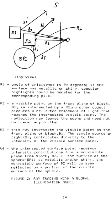
Rl

(Top

View)

-angle of inicidence is 90

degrees;

if the

surface was metallic or _shiny,

specular-highlights could be modeled for the

correspnding pixel

-a visible point on the front plane of

block,

B2,

is intersected

by

a R2;no other abject produces a reflected component of light that

reaches the intersected visible point. The

reflection _ray leaves the scene and need not.

be traced _any further.

R3 this _ray intersects the visible point on the

front plane of

block,

Bl. The single source of

light(S),

contributes

directly

to the

intensity

of the visible surface point.

R4 the intersected surface point receives

intensity

contributions from a nonvisible pi ame from

block,

B2. If the surface of the

sphere(SPl) is metallic and/or shiny, the

nonvisible surface of E<2 will be seen

reflected on a portion of the visible

surface of the sphere.

FIGURE 2: RAY TRACING WITH A GLOBAL ILLUMINATION MODEL

[image:22.528.87.441.19.658.2]

The global illumination _{model, using} the

intersection information from the _ray

tracing

_algorithm,

determines the

intensity

of the _{corresponding} pixels.

Ray

tracing

can support a _variety of _shading models and a

variety of geometrical descriptions of the? objects in the

scene.

In traditional ray

tracing,

for each _{ray reaching}

the viewer and

intersecting

a pixel on the screen

(SCANNING LEFT TO RIGHT AND TOP TO

BOTTOM),

a tree is

built. The nodes of the tree represent the ray-surface

intersections,and the branches represent any spawned,

reflected and/or refracted rays that might be modeled in

the shader. The

intensity

of a pixel is dependent on the

intensity

of light transmitted from the _{corresponding}

point on thie visible surface of an object to the viewer.

Among

the _contributing components that are modeled

by

the

illumination _model, are the reflected and refracted light

i-a_ys t hat r e a chi t hat _point. Contri but io n s of these 11 g h t

rays are based on the laws of optics [WHITSO, ROGE853.

The refraction and reflection rays are traced to their

r e s_pe ctj ve sources. These sources can be ot her surfac e s ,

or the light, source

(S),

and are assumed to be point

sources. If these -sources are other surfaces then the

to those point surfaces are also traced. This

tracing

of

the two light ray types continues until the light source

is _reached, or until the rays follow paths out of the

scene. These rays are traced backwards to the light

source (S) from the viewer. The shader then traverses the

tree from the leaves to the root _using the contributions

from the reflected and refracted surfaces, to determine?

the

intensity

of the pixel. The calculations _performed,

and the information maintained in the data structures

depend on the illumination model

being

implemented.

Regardless of thie illumination model _used, the _ray

tracing

algorithm must be able to extract the geometrical

information from the internal representation of the

objects, and determine the points, of intersection.

Different internal representations include approximation

by

polygons. The polygon is represented

by

an implicit

form of a. planar equation. In many implementations, the

ray is represented as a parametric equation. The two

points on the ray are the position of the

viewer-(PI) and

the pixel of current interest (P2) . The ray can be

defined as thus:

R =

RX

RY

RZ

P 1 -i- _{( F2}

= FIX + AT

= _P1Y + BT

- P1Z + CT

P 1 ) T

A :r _P2X -P 1 X

B == _F2Y - _{F 1Y}

C == _P2Z - _{P 1 Z}

The values for t are non-negative. This anchors the

ray at the viewer. Values less than zero are behind the

viewer and indicate intersection with objects not in the

scene. The parametric equations for x,y,z (RX,RY,RZ) are

substituted into the implicit form of the

planar-equation, and then solved for t. The value for t is

substituted into the parametric equations for RX,RY,RZ to

determine the actual intersection point. To make sure

that the intersection is within the bounded _plane, a

bounds test is performed. This same technique can be

applied to surfaces defined

by

quadric equations.

Here,

the quadratic formula is used to solve for t. A complex

root indicates no intersection. Reduction in time to do

intersection calculations with traditional ray

tracing

may be achieved by:

1-reducing the number of

intersection

calculations--a software _solution; or

2-using special-purpose hardware to shorten the time in

performing the intersection calculations EGLAS843.

2.2 I N T R 0 D U C T ION TO G Y S T 0 L I C A R R A Y S

Ray

tracing,

like many image? processing operations

performed o n pictures, is c o m_putat io n a_{1 J. y} inte n s i v e.

Calculations must be performed for each pixel. Special

pu r

-po s e a r chi i te ctu res have bee>_{n bui 1 1} to e x_ped i te thie I P

enhancement techniques EFU 823. Some of these special

purpose architectures are described

briefly

here. The

CLIP4 is 96 x 96 _array of parallel processors that

perform local neighborhood _{calculations,} such as shrink

and expand. The processors can be reconfigured

by-different types of neighbor connections (I.E. 6-CQNNECTED

OR 3-CONNECTED) . The _mpp (MASSIVELY PARALLEL

PROCESSOR),

built

by

Goodyear Aerospace Co. for NASA ,consists of 256

processing elements, which _may contain _up to 32

processing units. The MPP was designed to perform IP

functions,

such as feature _extraction, pattern

recognition, and relaxation. The ILLIAC IV is a SIMD

architecture with one central control _unit, and 64

processing units, and was designed to handle a range? of

problems. The IF'

appl ications include _clustering, pattern

classification arid texture analysis.

Picap

II is a MIMD

architecture that allows _up to 64 x 64 neighborhoods in

performing pattern recognition calculations on multiple

images. Measurements are _{automatically} performed on a

field of data that is 512 x 640 to reduce the input. The

measurements include histogram collection, gray scale?

range

determination,

and _x-y extent determination. In

addition, there are dedicated processors for performing

filtering, generating graphical _overlays, and for

labeling

and template _matching CFU--823.

Also,

extensions

to _{existing programming} languages have been implemented

to reflect these new _{architectures,} and to facilitate the

development of algorithms to take? advantage of the new

architectures. For the

CLIP4-array processor, an

extension of Pascal _, i. e. _{Pascal pi,} has been implemented

[UHRB23. Applications that have been implemented using

this language include _performing calculations in

IF',

pattern recognition and scene description. Constructs of

the language include parallel _{assignment, condition,} and

i /o statements as well as; parallel _{proceedures, allowing}

for-the simultaneous _processing of _{array elements,} as

well as sets of arrays. The data types of these arrays

are

binary,

_gray scale, or nonnumeric.

Also,

the

capability exists to access relative locations in a two

dimensional array in order to perform _operations, such

as, windowing and _masking C DUFFS XI , UHR843. PPL (PICTURE

PROCESSING LANGAUGE) developed for the

F'icap

I and _{Pi cap}

II is also an extension of Pascal. Features of the

language to facilitate the image

pi-ocessi_ng computation:.

in c1ude bi n ar_{y p i}ctur e_{, p i}ctu_re, and te m_{p 1}ate eiem ent as

data, types. Picture operators include? parallel arithmetic

operations on 3x3 neighborhoods [DUFFS! 3. One of the

languages includes Pixal (PIXEL MANIPULATION ALGORITHMIC

LANGUAGE) , also targeted for the

CLIP4,

is an extension

of Algol60. D<*ta types specific to IF include grey,

binary,

mask and frame. Control structures tailored for

IF'

include parallel assignment _statements, parallel

comparisons between _masks, and submatrici es of a two

dimensional _array, and parallel arithmetic operations.

Pixal has been used to implement parallel

thinning

and

object extraction algorithms [DUFF81 , FU823,,

IP has _recently found

help

for its calculations from

the VLSI (VERY LARGE SCALE INTEGRATION)

technology

in the

form of systolic based architectures CKUNGB23.

Currently,

VLSI on a single _chip is a two dimensional

technology,

that

is,

architectures are designed and laid out in a two

dimensional grid. Problems arise when there is too much

crossover of communications paths between the cells

[JALA853. To reduce crosstalk it is neccessary to have

short and regular paths on the chip, in order to reduce

the initial design cost and delays

during

execution.

These two dimensional architectures are easier and

cheaper to manufacture when the cells/components

of-the

chip are of regular shapes with regular interconnections.

The s.i~ravs may be one dimensional or two ci i.moiisionaJ _,

depending

on the algorithm to be implemented.

Systolic a chiteetui es exploit t:it-?se constraints to

make algorithms, that can also exploit tnese constraints

a specialised architecture that embeds much of the

algorithm in the hardware. Applications for systolic

architectures have included IP _operations, matrix

arithmetic _operations, data base _{manipulations,} speech

recognition _{systems, vision,} and stero vision systems

LK1JNG82,

MEAD80,

FRIS85,

GUER85_, SYMA850. The design

principles of systolic architectures are descr 1nod belcu

A single cell is replaced _by an _array of cells CKUNG82 3.

T h isi a1 1c? w s t.hie t hir o u_{g h p}ut to be in c r e a s e ci wiehio ut

increasing

the? _memory bandwidth. One of the? goals of

systolic architectures is to decompose complex problems

into simple and regular pieces that can _map onto regular

simple, arid _relatively fast cells. These cells per form

the specialized calculations, and have the same? design.

The throughput of the system is tnen improved

i.y

also

implementing

concurrency to the extent permitted

by

the

algorithm. In a systolic archi tec tun

>.._-, tnie :.s

accomplished

by

"pumping"

i.ho data through the cells.

Once art input value has been useci in a _calculation, the

data is passed on to the next cell. The next cell is

algorithm dependenc This; circulating of data imposes a

regui. ar flow of data throughout the system, arid enables

the simultaneous execution of many cells. The regular

njiiimunicdtion paths for the data reduce the overhead

of the systolic architecture is; to balance the

computational bandwidth with the I/O bandwidth. Once a

data item has entered the _array, the data is reused. The

data are input to the

boundary

ceils of the array

[KUNG823.

Therefore,

the criteria used to determine

whether an algorithm is amenable to execution on a

systolic based architecture appear to be the following:

1- _{the algorithm is compute bound rather than}

I/O bound (.I.E,THE NUMBER OF

NUMBER OF I/O DATA

ELEMENTS);

I/O bound (.I.E,THE NUMBER OF OPERATIONS EXCEED THE

2-the algorithm must execute in real-time

(I.E.,

WHILE THE USER VIEWS THE IMAGE ON THE

SCREEN);

3- _{the calculation are regular} and can be;

defined with simple recurrence relations;

4- _{the design}

of the components on the _chip to implement

the algorithm aie regular

(I.E. ,MINIMIZE CROSSTALK AND DESIGN COSTS) [JALAS53.

1.3 APPLICATION OF SYSTOLIC ARCHITECTURES FOR RAY TRACING

2.3.1 RAY TRACING AS A HIDDEN SURFACE REMOVAL TECHNIQUE

2.3.1.1 POLYGON APPROXI MAT I ON

The _ray

tracing

algorithm can be adapted to take

advantage of the VLSI systolic technology.

Starting

with

ray

tracing

as a visible surface algorithm, and with the

solid objects in a scone approximated with _polygons, the

the? traditional _ray

tracing

algorithm can be reduced

by-adapting the algorithm

to,

and

by,

_running the _algorithm,

on, a systolic: based architecture?. The _ray

tracing

algorithm meets the criteria stated in the previous

section (SECTION 1.2). The ray

tracing

algorithm is

certainly compute bound with each pixel _ray

being

compared to each polygon in the scene. Back plane _culling

could be used to remove those polygons that are

obviously-hidden from the? viewer. The picture must be generated in

real_{-time, especially} when _ray

tracing

is a part of a

solids modeler of a CAD/CAM workstation. Although there

are no recurrence _relations, the same calculations are

done repeatedly for each pixel in the _screen,

for-each

plane in the scene. For ray-plane

intersections,

the

calculations are strai ghtf orward. Since the cells must

perform the same calculations, and the pixels are scanned

in an incremental order, the? design of the cells should

be the same. The interconnections-, between the cells;

should be linear rather than

diagonal,

vertical, or

horizontal as in IP- This type of connection is certainly

regular. The number of pixels that need to be intensified

or shaded is proportional to an area on the surface of

the graphical

display

device. The area is normally

rectangular. The complexity of the scene and of the

objects would determine the

approximate the objects. The systolic architecture to

implement the ray

tracing

algorithm is based on the

calculations that must, be performed. The calculations

that must be performed are the _{intersections} of a

directed line segment with planes. The general form of a

p 1an ar _equation is :

AX +

BY + _CZ + _D =: ₀

The parametric form of the x,y,z components of the _ray

are: (VIEWER POSITION DENOTED BY XO,YO,ZO)

X (T) = _XO + _ET Y(T) = _YO + _FT Z (T) = _ZO + _GT

The right side? of the equations are substituted into the

plane equation:

A(XO + ET) + Bi'YO + FT) + C(ZO + GT) + D -0

Then the equation is solved for ts

t = _-(AXO + BYO + CZO + D) / AE + BF + CG

WHERE: AE + BF + CG is NOT EQUAL TO ZERO

The value of t can be checked to make sui e that it

is _positive, and that the point of intersection is in

front of the viewer. If positive, the value of t is

s ubsti tuted back: into the par

-a m etnc: equations for t he

x,y,z components of the ray. A rectangular bounds test is

performed for each

bounding

plane to make sure that the

intersection point is within the bounded planes that are

part of the object. The

following

set of equations must

be? _{simultaneously} satisfied,,

XMIN

YMIN

ZMIN

X <> XMAX

Y <= _YMAX

Z <== _ZMAX

For _{visibility calculations,} the pixel can be

intensified to the color of the polygon, or to the

background_, if there are no valid intersections. The

colors available are dependent on the capabilities of the

graphics processor in the

display

terminal. Normal

1/,

some method is provided to specify the varying

intensities of _red, green and blue to generate the

desired color for the pixel. The data for _calculating

t,

the coefficients of the plane, the? position of the

viewer, and the current pixel to be

intensified,

are

readily available. A systolic array of

linearly

connected

cells that can support the calculations is shown in

Figure 3. The number of cells (M) is equal to the number

of polygons in the scene. The inputs and the outputs of

the cells are the pixel coordinates, the line parameters

of the ray, a t parameter _value, and a polygon

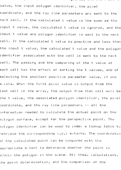
identifier. At the start of the intersection calculation,

used to calculate the t for the cell. If the calculated t

value is _negative, the value is

ignored,

and the input t value, the input polygon

identifier,

_the pixel

coordinate, and the ray line parameters a.re sent to the next cell. If the calculated t value is the same as the

input t _value, the calculated t value is

ignored,

and the input t value and polygon identifier is sent to the next cell. If the calculated t value is positive and less than [image:34.528.64.469.69.639.2]

the input t _value, the calculated t value and the polygon

identifier associated with the cell is sent to the next cell. The _passing and the _comparing of the t value at

each cell has the effect of _sorting the t _values, and of

selecting the smallest positive parameter _value, if one

exists. When the first pixel value is output from the

last cell in the _array^ the output from that cell will be

the t _value, the associated polygon

identifier,

the pixel

coordinate, and the ray line parameters all the?

information needed to calculate the actual point on the

polygon _surface, except for the perspective point. The

polygon identifier can be used to index a

lookup

table to

retrieve the corresponding x ,y,z extents. 3"

he? coordinates

of the c a1c u1 a.te ci _point ea. n be co m pared withi the

a_{p p}

|-o_pr i.ate e,-.te nt to dete r min e whet her thie point i s

within the polygon in the scene. All these _{calculations,} the _point determinat

ion,

and the c o m parison of the

c oordinate s wi t hi the e :;te nts_, c a n hie pe i

-far m ed

by

a

separate, single cell. Depicted as S in Figure 3. The

output of this cell is the intersection point and the

polygon identifier , or a not valid intersection

indicator-. This i1 1fo r m at io n is cir c u1ated t hir o u_{g h} t he

systolic _array, or sent

directly

to the interface buffer,

Figure 3 depicts a high level representation of the

supporting architecture. The operations performed

indicate a need for local _memory to sitore? intermediate

results.

The architecture of a cell is based on the _assembly

language level_like

calculations found in Appendix D

Figure 4 shows the architecture designed to support the

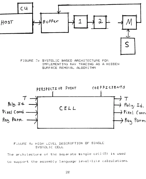
FIGURE 3: SYSTOLIC BASED ARCHITECTURE FOR

IMPLEMENTING RAY TRACING AS A HIDDEN

SURFACE REMOVAL ALGORITHM

T

M

pol^jd.

}

P'ixe[

Coo*!.

Ra^

far/n.

pEdSPEtTioe

p0Lur

coefficients

Mt

P'Uel

Coord.

Irm.

FIGURE 4: HIGH LEVEL DESCRIPTION OF SINGLE

SYSTOLIC CELL

Trie architecture of the separate single cell(S) is used

to su_{p p}ort thie a. s s e mb_{1 y} lan_gu a_ge 1e v e1

-11 1-.e calcu1ations

[image:36.528.30.515.75.668.2]

found in Appendix D. Figure

the single separate cell.

shows the archiecture of

S'm^lc

JcpavQ-ir.

Cell

fWfecfii/e

FIGURE 5: HIGH LEVEL DESCRIPTION OF A

SEPARATE CELL PROCESSOR

One consequence of _using the systolic based architecture

is the _{necessary mapping} of the algorithm onto this

hardware. A high level description of the algorithm is

gi ven here:

PICK A PERSPECTIVE POINT

FOR. EACH PIXEL IN THE VERTCAL DIRECTION

FOR EACH PIXEL IN THE HORIZONTAL DIRECTION

FOR EACH FOLYGOM IN THE SCENE

DETERMINE RAY PARAMETERS

CALCULATE INTERSECTION POINT

END FOR

END FOR

END FOR

The language in which tins algorithm is implemented

must be _enhanced, or designed, to accommodate the net-,)

code that must be generated. This implies that the

compiler designer must be

knowledgeable

about the

underlying auxiliary systolic architecture. The _scanning

of the

display

1eft

to-right ,

top--to-bottom , suggests a

data type in the language that is _{automatically} accessed

in the same _manner, and is _{rectangularly} shaped. As this

data structure is _scanned, the pixel coordinates can be

generated with the ray parameters, and sent to the

systolic array.

Normally,

a special purpose _{architecture,}

like the systolic _arrays, is connected to a

traditional,

general purpose?, host computer. Based on the above

algorithm, and on the calculations that must be

performed, the parameters that, must be made available at

the? time the systolic _array iss _ready to perform the

intersection calculations are shown here:

. STARTING PIXEL LOCATION

. NUMBER OF PIXELS IN THE HORIZONTAL AND VERTICAL

DIRECTIONS

. POINT OF VIEW

. POLYGON IDENTIFIER

. COEFFICIENTS OF PLANE EQUATION

T hie 1a st ite m in the list will de_pe nd o n t hie

internal description of the objects in the scene. The

inter n a1 de sc ri pcion is de_pe ndent on the m at. hiem a11 c a1

-functions used to depict the scene objects,, For the

the planar _{coefficients,} the x,y,z _extents, and the

polygon identifiers _quickly from the internal data

structure. The interface between the host and the

systolic _array is a _memory buffer with separate input anc

output _ports, between the host and the buffer _, and the

array and the buffer. Before the calculations

begin,

the

planar coefficients must be preloaded into the cells, as

well _as, the x,y,z extents, and the perspective point

into the

lookup

table,

and the single separate _cell,

respectively. An _entry of the

lookup

table is as shown

here:

Poll).

-i

K

1)

Z

tXTBWS

Fitfei

Locaf'/or)

The format of the data stream _coming from the

buffer-would be:

A1B1C1D1X1Y1Z1P0LY1

. . . . AMBMCMDMX-MYMZMPOLYM*

Where the '#'

is an end-of-datastream indicator". The

instructions to be executed should also be preloaded

EUME0853. The format of the data stream should be:

I1+I2-+I3+. . . +IK

Where?:

k

-number of instructions

+

-an interi n struct! on indicator

--

end-of-instruction stream indicator

Ther^e instructions could be sent through the cells

like the

data,

or be broadcast

by

the host

directly

to

the cells. The microcode should be extremely fast. The

instructions need _only be loaded canoe. The idea of

loading

instructions suggests howi systolic arrays can be

tailored tc? accommodate different, surface-ray

calculations. This would also require the _preloading and

circulating of different data values. Once the _necessary

corresponding ray paramemters must be? _generated, and sent

through the systolic array. _{For hidden}

surface _removal,

the pixel parameters need _only be sent through the

systolic _array once. There will be an initial

delay

until

the first t value is output from the last cell.

Then,

the

a r

-r a_y she u1 d o u_{t p}ut t values at r e_qu1a. r inte r v a1s.

2.3.1.1.1 ANALYSIS OF THE USE OF SYSTOLIC ARRAYS

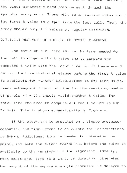
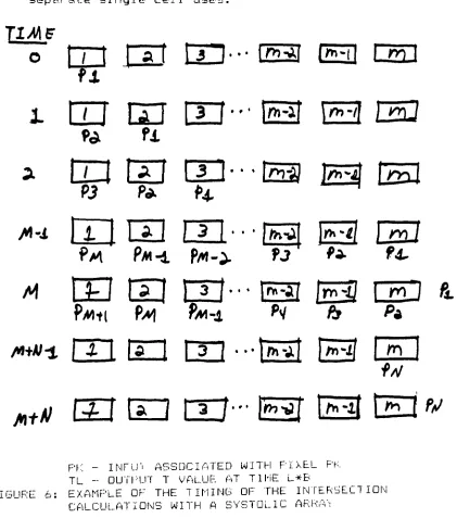
The basic unit of time (B) is the time needed for

the cell to compute the t value and to compare the

computed t value with the input t value. If there are M

cells, the time that must elapse before the first t value

is available for further calculations is M*B time units.

Every

subsequent B unit of time for the _remaining number

of pixels (N

-1) _, should yield another t value. The?

total time required to compute all the t value's is B*M -r

B*(N-1). This is shown _{schematically} in Figure 6.

If the

algorithm-1 is executed on a single

processor-computer _, the time needed to calculate the intersections

is Ef*N*M. Additional time is needed to determine the

po

int,

a n ci it iahe t he e xter11 c o mpa rions before t he _point i s

available to trie remainder of the algorithm.

Ideally,

this additional time is B units in

duration,

otherwise.' [image:41.528.60.472.61.620.2]

the next multiple of B. The

delay

requires the queuing of

the pixel _coordinates, the ray parameters, the t _value,

and the? polygon identifier. The number of entries in the

queue is proportional to the number of B units the

separate single cell uses.

o

fT~t

psi

rri"-

p^

geeo

Hvfi

i

tZJ

DlJ

CEJ-"

\EH

\EI

CS2

*

tn izj

tx3---isa

a

ta

Pi

P*

*

^

/1-1

Pm

Pm-i

P/h->

?j

'*

f4.

m

ES

CEJ

nEJ-"

ESI

Ie3

rFn

&

P/Mtl

PaI

Bm-i

pv

&

**

^

GET

CO

CH-S

E3

S

w

PK _ IMFU"' ASSOCIATED WITH PIXEL F'K

TL - _OUTPUT T VALUE AT TIME L*B

FIGURE 6: EXAMPLE OF THE TIMING OF THE INTERSECTION

[image:42.528.54.475.131.608.2]

2.3.1.2 QUADRIC SURFACES

Quadric surfaces are exemplified

by

the conic

sections ( I E. ,CIRCLE,

ELLIPSE,

PARABOLA,

AND HYPERBOLA)

extended to three dimensions. A quadric surface is of the

form:

DX-**2 + BY*-*2 + FZ**2 + GXY + HXZ + IYZ + YX +

KY + L.Z + M = _{0 (1)}

This expression is also an implicit _equation, in

which thie parametric components of the _ray can be

substituted for x,y,z.

Recalling

the parametric, form of

t he r a_y :

X (T) ^ _XO + _A*T

Y(T) = _YO

-i-B*T

Z (T) = _ZO + C*T

Subst

ituting

into e_qu at ion ( 1 ) :

D(XO

T-A*T)**2 -i- _EI*

(YO + B*T)*₂ -+ F-*(20 + C*T)**2

I-MYO + A*-T)#(ZO + C*T) +

J*(XO + A*T)

+-K*(YO + _B*T) + L*(ZO + _C*T) + M = ₀

Expand! ng:;

D* _{(Y 0}* *2 + _A**2T*-2

+-2*_{X 0 A}*_{T )} +

E*<Y0**2 + _B**2T**2 + _2*Y0#B*T>

->-F-*(Z0**2 + _C**2T**2 + _2*Z0*C*T) +

G*iXO*YO + _T*(XO*B + YO*A) + _A*B*T**2) +

H*(XO*YO + _T*(XO*C

h-ZO*A) + A*C*T**2) +

I*(YO*ZO + _T*(YO*C + ZO*B) + B*C*T**2) +

J*(.XO + _A*T) + K*(YO + B*T) + L*(ZO + C*T) + M = ₀

And collecting like powers of t yields:

T**2 (D*A**2 + E*B**2 + _F*C-<-#2 -+

G*A*B + H*A*C + I*B*C ) +

T*(2*D*A*X0 -i- _2*E*B#Y0 +

2*F*C*Z0 + G*(XO*B + YO*A.> +

H*(XO*C + ZO*A) + I*(YO*C +Ze*B..' +

J*A + f>B + L*C ) +

(D*Xu**2 + E*Y0**2 + F*Z0**2 + G*XO*YO + H*XO*ZO + I*YO-*ZO +

J*XO + K*YO + L*ZO -+ M )

= _{0 (3)}

Equation (3> is in the form:

A '

-*T-*-*2

-i-B *T -i- _C

-0;

The values of t can be solved

for"

by

using the quadratic

T - ( -B

' -r/~

( B '**-2

-4*_{A *C')**l/2 ) / 2*A}

The coefficients are based on the perspective _point,

and the _ray parameters and coefficients of the quadric

surface. Complex values of t indicate no intersection

with the _surface, and can be ignored.

Again,

negative t

values can also be

ignored,

because the intersection

point is not within the scene. Since there are two t

values _generated, the smaller positive t value is chosen.

The t value is put back into the ray component equation

to determine the point on the surface. A bounds test is

made to ensure that the point is, within the? sight of the

vi

ewer-.

The architecture _supporting the intersection

calculations, is a one dimensional _array of connected

cells, one cell for each surface in the scene. The

systolic _array communicates with the host via an

interface buffer.

Preprocessing

prior to the intersection

calculations include? generating the pixel. cca

dinuteb,

and _computing the _ray parameter and surface? coefficients.

The pixel coordinates are generated a second time when

the coordinates are sent through the array. The inputs

its _ray parameters, a t _value, and a surface identifier

The two t values are generated through the quadratic

fo r mula. Ea chi c e1 1 _pe rfo r m s t he a s s e mI:?_{I y} 1an_gauge

level-like operations found in Appendix D.

The _supporting architecture is shown in Figure 3.

The determination of which t value is sent to the next

cell is shown in the high level algorithm here:

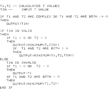
T1,T2 CALCULATED T VALUES

TIN INPUT T VALUE

IF Tl AND T2 ARE COMPLEX OR Tl AND T2 ARE BOTH -> 0

THEN

OUTPUT (T IN)

IF TIN IS VALID

THEN

IF Tl > 0 OR T2 > 0

THEN

OUTPUT( M I N I MUM ( T,T I N ) )

IF Tl AND T2 ARE BOTH > 0

THEN

OUTPUT (MINI MUM ( T 1 ,T2,T I N ) )

ELSE

TIN IS INVALID

IF Tl > 0 OR T2 > 0

THEN

OUTPUT (T)

IF Tl AND T2 ARE BOTH > 0

THEN

OUTPUT( M I N I MUM ( T 1 ,T2 ) )

END IF

The output from the last cell includes trie smallest

positive t

value-if there is one--the _{corresponding}

[image:46.528.73.453.231.550.2]

parameters. The separate single cell performs the same

basic calculations as for polygon approximation. The t

veUue is substituted into the parametric _ray equations to

determine the point on the surface, the surface

identifier is used to index a

lookup

table to retrieve

the x,y,z extents. The x,y,z coordinates are compared

with the extents. The output of the separate? single cell

is an intersection point and a surface _identifier, or"

an

intersection point and an invalid surface indicator.

Again,

the output can be circulated through the _cell, or

sent

directly

to the interface buffer. The algorithm that

must be mapped onto the? systolic _array is shown below:

PICK A PERSPECTIVE POINT

FOR THE NUMBER OF PIXELS IN THE VERTICAL DIRECTION

FOR THE NUMBER OF PIXELS IN THE HORIZONTAL DIRECTION

DETERMINE THE RAY PARAMETERS

FOR EACH SURFACE IN THE SCENE

PERFORM RAY-SURFACE INTERSECTION

CALCULATION

END FOR

DETERMINE SURFACE POINT

COMPARE WITH SURFACE EXTENTS

END FOR

END FOR

The a_{I g}or

-11hm as s uin es a ho mo_ge? n e o u s seen e_; that is,

all the objects in the scene are represented as quadric

start of the intersection calculations is similar to the

information that must be available for polygon

approximation of a scene. The list of information is:

. STARTING PIXEL COORDINATE

. NUMBER OF PIXELS IN THE HORIZONTAL AND VERTICAL

DIRECTIONS

. PERSPECTIVE. POINT

. INITIAL SURFACE IDENTIFIER AND T _VALUE

. COEFFICIENTS OF THE QUADRIC SURFACE

The initial surface identifier is an invalid _one,

and the t value is negative. These initial values are

implementation

dependent,

and indicate that the ray does

not intersect _any object in the scene. Once the? _ray has

circulated through the? systolic _array, the surface

identifier and t value will either still indicate that.

the _ray does not intersect any object in the _scene, or

the closest

intersecting

surface and the? parametric

intersecting

t value?. The instructions to perform the

intersection calculations are loaded

during

the?

preprocessing of the surface coefficients, using the same

fo r

-ni at a s de s c r i be cl for- _po_{1 y g}on a_{p p}r o xim at io n of a s c e n e.

The coefficients are broadcast to the appropriate ceils.

Again,

there will be an initial delay until the first t

v alue is a v aiIab1e.

2.3.1.2.1 ANALYSIS OF USE OF THE SYSTOLIC ARRAYS

The basic unit of time (B) is based on the computing

of the t values with the quadt atric

formula,

and the

comparing of the t values for the smallest positive

value. The _qu adi~

ic s u rfaces a re mo r e c o m_{p 1}e x t hia. n thie

planar _polygons, and require more time to determine the t

value to output to the next cell. The variability in time

comes from the square root calculation and the comparison

of the t values. The? square root can be calculated

by

using an iterative _algorithm, or retrieved from a

lookup

table. The number of iterations can not be _{predetermined,}

and is based on the desired number of digits of _accuracy.

The

lookup

table removes this variability, but requires the generation of a globally accessible data structure.

The other source of variability with respect to time is

the comparison of the t values. Upon the selection of the

t value to be input to the next _cell, the cell _may be

idle until the B unit of time has elapsed.

The intial

delay

until the first t value is

available is as before: M*B, where M is the number of

cells <ICE., THE NUMBER OF"

QUADRIC SURFACES). The

subsequent t values are available _every B units for the

remaining pixels (N-l). The total time that must elapse

before all the t value's are available is:

M-fc-B +

(N -1)*B = _B*(M + N

-1).

The time needed to perform the actual point _{calculations,}

and the extent _comparisons, is the same length as for the

polygons. If the time to make these calculations is

L,

the time that must elapse before the surface point is

available to the remainder of the algorithm is M*B + L.

The total time that must elapse before all the points are

available to the algorithm in the host is:

M*B + L + _(N-l) (E + L) = _B*(M + N -1)

For execution on a single processor computer-the

analysis i- as follows. Thie total time that must elapse

before the first t parameter is available is M*B + L. The

total time that must elapse before all the intersection

points are available issN*(M*B + L) == _N*M*B + N*L.

Calculations are based on the

following

high level

aIgorithm:

FOR ALL THE PIXELS(N)

FOR ALL THE OBJECTS (M)

CALCULATE THE INTERSECTION POINT (B)

END FOR

DETERMINE ACTUAL SURFACE POINT (L)

END FOR

Since the time to determine the actual surface point

is the same as for polygon _{approximation} of the _scene,

and the basic unit of time to perform the t calculations

is

longer,

the number of input t values to the separate

single cell that must be queued should be smaller than

for polygon

approximation,

or non-existent.

2.3.1.3 COMPOSITE SOLIDS

2.3.1.3.1 CONSTRUCTIVE SOLID GEOMETRY SOLIDS

Ray

tracing

has been used to synthesize objects

built

by

solid _modelers, in _particular,

by

constructive

solid _geometry (CSG) modelers

[R0TH82,

WYV.I86,

CASA85,

F'LUN853. A constructive solid modeler (CSG)

modeler-builds _up an object from a set of primitive solids that

are combined hierarchi al_{1 y} in a

binary

tree with boolean

operators. The primitive objects

typically

are:

block,

sphere, cylinder,

torus,

and cone. The regularized

boolean operators are union,

intersection,

and

d i f ference.

The

binary

tree consists of the primitive solids as

t hie 1e a v e s , and t he in te rior nod es a. r e t he bo o1e a n

operators. The root node represents the final object.

Ea cI"i l nte rio r

-n ode r e_pr e s e nts a boa1e a n oper at ion_, o r a

r_{i g i}d bod y m otion s u ch a s tr an s1at ion a nd r otat

ion,

t hat

is -a_{pp lie d} to the c o r

i-e s_po nd ir i_g s ub tr e e. W hen a object is

rendered with ray

tracing,

each _ray must traverse the

binary tree,

representing the _{object, starting} at the

root. The intersections of the straight line ray with the

primitive _{objects, making}

up the composite _object, are

c aleu1ated _, and t hie r a_y is s ubclivided into regions t hat

are _{outside, on,} or inside the boundaries of the solids.

The _ray is; a parametric equation of a line? anchored at

the _viewer, and directed toward the scene. When the

inter-section calculations with a solid primitive have

been performed, the results are combined with the results

of the other branch from the same parent _{node, according}

to the boolean operator in thie parent node. This

information _along with an ^identification of the

intersected surface is maintained in a global data

structure?. The results of one level are combined and

returned to the next higher level in the tree? until the

r oot i s r eached.

The sides of a block are usually represented as six

half planes. The sphere, cylinder, and cone are examples

of quadric _surfaces; the torus is represented

by

a

quartic polynomial. The different representations

imply-that different calculations are needed to accommodate the

different surface

types,

and these calculations require a

different amount of time.

Also,

the hierarchical

relationships _among the primitive solids must be

maintained. Both of these

features

of CSG solids preclude

the

beneficial

use of a one

dimensional

systolic _array to

perform the

intersection

calculations,, The _uniformity

criteria for qualification for execution on a systolic

array can not. be? met.

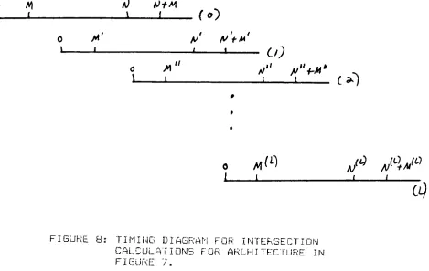
2.3.1.3.2 HETEROGENEOUS SCENE

A scene _consisting of surfaces of different

mathematical (ANALYTICAL) representations can be rendered

with a systolic based architecture to facilitate the

intersection calculations,, The systolic based

architecture consists of a number of one dimensional

arrays. Each cell of the systolic _array calculates the

intersection for a particular surface type. The length of

eachi _array is equal to the? number of objects in the scene

with the same mathematical representation. Each cell of

the _array is preloade?d with the corresponding

instructions to perform the? intersection calculations,

and with the coefficients of one object in the scene? with

the representation corresponding to the array. The basic

unit of

time,,

the? time to perform one intersection

c a1c u

lation,

is cli f fer e nt fo r e a chi a.r r a_y. T hi is c! if fe r e n c e

in time for the intersection calculations must be

resolved before the systolic based architecture can be

used.

The systolic arrays should be arranged in

decreasing

or

increasing

time to perform the intersection

calculations. If the arrays are sorted in _increasing time

to perform the intersection _{calculations,} the circulated

t values, and _ray parameters generated from one

array-will queue _{up waiting} to circulate through the next

slower array. The length of the queue depends on the

relative slowness of one _array with respect to a previous

array,, This arrangement of the arrays ensures that each

array is in continuous _operation, once the the values

enter the _array, but also requires more _memory to hold

the _qu eued in_puts. T hie a1 1e r n at iv e ar r a n_ge m e nt 1 s to

order the arrays in

decreasing

time of the intersection

calculations. The subsequent arrays require a shorter

time interval to calculate the ray-surface intersections.

As a _consequence, the subsequent arrays will not be

continuously active?. The previous arrays will generate? t

values at. a rate slower than the next array, and,

therefore,

no _memory is needed to hold intermediate

results. The? time interval between consecutive? inputs to

an _array should become shorter, as subsequent arrays

became _active, and consequently each array must have its