MICRO-MACRO MODELING OF ADVANCED MATERIALS BY
HYBRID FINITE ELEMENT METHOD
by
Changyong Cao
A thesis submitted for the degree of
Doctor of Philosophy
of The Australian National University
Thesis Supervisors:
Prof. Qinghua Qin Prof. Aibing Yu
Supervisory Panel:
Prof. Qinghua Qin, The Australian National University, Chair Prof. Aibing Yu, The University of New South Wales
Prof. Xi-Qiao Feng, Tsinghua University, China Prof. Xuanhe Zhao, Duke University, USA
iii
Declaration
I hereby declare that this submission is my own work at the Research School of Engineering of The Australian National University, Canberra, Australia. This thesis contains no material that has been previously accepted for the award of any other degree in any university, and contains no material previously published or written by another person, except where acknowledged in the customary manner.
I also declare that the intellectual content of this thesis is the product of my own work, except to the extent that assistance from others in the project's design and conception or in style, presentation and linguistic expression is acknowledged.
(Signed) Changyong Cao
Dedication
v
Acknowledgements
During the long journey of my PhD study over the past few years, many people have supported me in different ways. This is a right moment that I would like to give those people sincerely gratitude. First I would like to express my deepest gratitude to my thesis supervisors Professor Qinghua Qin and Professor Aibing Yu for their great support, inspiring guidance and kind encouragement to me during my study, especially in difficult moments. Their breadth of intellectual inquisition continually stimulates my analytical thinking skills. This work would not have been accomplished without their efforts. I am deeply indebted for their guidance and support in both my study and my daily life.
I sincerely thank my committee members for their continuous effort, valuable insights and kind willingness to serve in my supervisory committee. In particular, I would like to thank Professor Xi-Qiao Feng for his guidance on instability analysis and modeling of biomaterials during my stay at Tsinghua University. I am deeply impressed by his enthusiasm as to the various scientific researches. His dedication to science has inspired me to be a scholar in mechanics for which I owe much gratitude.
I would like to express my sincerely gratitude to Professor Xuanhe Zhao of Duke University for his kind guidance, strong support and fruitful discussion. I have benefited significantly from his teaching and mentorship on mechanics of soft active materials. He taught me many wonderful things about mechanics, offered me much sound advice, and helped me get through difficult times. I am grateful to Professor Zbigniew Stachurski for his discussion and guidance in the topic of composite materials. I would like to thank Professor Shaofan Li for his hosting, support and discussions during my research visit to the University of California at Berkeley.
Hui Wang for his valuable suggestions and fruitful discussion during his visit to ANU. I would like to thank my colleagues Mr. Jin Tao, Mr. Zewei Zhang, Mr. Check Yu Lee and Mr. Song Chen for their help, discussion and company during my study at ANU. Special thanks are also due to my friends Mr. Wensheng Liang, Ms. Ting Cao, Mr. Zhuojia Fu, Dr. Yongling Ren and Mr. Yimao Wan from ANU for their help and the wonderful times we had together. I would like to thank Mr. Xiaoyu Sun for his great help during my stay at Tsinghua. Thanks also to Ms. Weihua Xie, Mr. Mangong Zhang, Mr. Cheng Ye, Dr. Yue Li, Mr. Liyuan Zhang, Ms. Xiangying Ji and many other friends from Tsinghua, and Mr. Honfai Chan, Mr. Stephene Ubnoske, Mr. Qiming Wang and Mr. Qing Tu from Duke. I sincerely thank our supporting staff at
CECS, especially Mr. Jonathan Peters, Ms. Kylee Robinson and Ms. Suzy Andrew. I would like to extend my thanks to all the friends, colleagues and staff at ANU, Tsinghua, Duke and UC Berkeley for their help and for creating a pleasant working atmosphere.
I greatly acknowledge the International PhD Scholarship and HDR Merits Scholarship from ANU, and research funding from Laboratory for Simulation and Modeling of Particulate Systems at UNSW for providing financial support during my PhD study. My research visit overseas and conference attendance were also funded by Vice Chancellor’s Travel Grants and Dean’s Travel Grant from ANU.
vii
Micro-macro Modeling of Advanced Materials by Hybrid Finite
Element Method
by Changyong Cao
Research School of Engineering, Australian National University, 2013
ABSTRACT
Advanced composite materials are increasingly used in a variety of fields due to their desirable properties. The use of these advanced materials in different applications requires a thorough understanding of the effect of their complex microstructures and the effect of the operating environment on the materials. This requires an efficient, robust and powerful tool that is able to predict the behavior of composites under a variety of loading conditions. This research addresses this problem and develops a new convenient numerical method and framework for users to perform such analyses of composites.
the proposed micromechanical models. Meanwhile, special elements are also proposed for mesh reduction and efficiency improvement in the analyses.
ix
Table of Contents
List of Tables... xv
List of Figures ... xvii
Chapter 1. Introduction ... 1
1.1. Background and motivation ... 1
1.2. Modeling of advanced materials ... 2
1.2.1. Macroscale modeling of composites ... 2
1.2.2. Microscale modeling of composites... 4
1.2.3. Multiscale modeling of composites ... 8
1.2.4. Modeling of multifield materials ... 9
1.3. Hybrid finite element method ... 11
1.3.1. Hybrid Trefftz finite element method ... 11
1.3.2. Hybrid fundamental solution-based finite element method ... 14
1.4. Objectives of research ... 15
1.5. Scope and organization of thesis ... 16
Chapter 2. Framework of HFS-FEM for Plane Elasticity and Potential Problems ... 19
2.1. Introduction ... 19
2.2. Formulations of HFS-FEM for elasticity ... 20
2.2.1. Linear theory of plane elasticity ... 20
2.2.2. Assumed fields ... 22
2.2.3. Modified functional for the hybrid FEM ... 25
2.2.4. Element stiffness equation ... 26
2.2.5. Numerical integral for H and G matrix ... 27
2.2.6. Recovery of rigid-body motion ... 28
2.3. Formulations of HFS-FEM for potential problems ... 29
2.3.1. Basic equations of potential problems ... 29
2.3.2. Assumed fields ... 29
2.3.3. Modified variational principle ... 31
2.3.4. Element stiffness equation ... 34
2.3.5. Numerical integral for H and G matrix ... 35
2.3.6. Recovery of rigid-body motion ... 36
Chapter 3. HFS-FEM for Three-Dimensional Elastic Problems ... 38
3.1. Introduction ... 38
3.2. Formulations for 3D elasticity without the body force ... 40
3.2.1. Governing equations and boundary conditions... 40
3.2.2. Assumed fields ... 41
3.2.3. Modified functional for hybrid FEM ... 44
3.2.4. Element stiffness equation ... 45
3.2.5. Numerical integral over element ... 46
3.2.6. Recovery of rigid-body motion terms ... 48
3.3. Formulations for 3D elasticity with body force ... 49
3.3.1. Governing equations ... 49
3.3.2. The method of particular solution ... 49
3.4. Radial basis function approximation ... 50
3.5. HFS-FEM for homogeneous solution ... 51
3.6. Numerical examples... 52
3.6.1. 3D Patch test ... 52
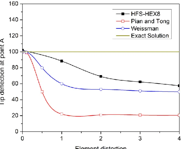
3.6.2. Beam bending: sensitivity to mesh distortion ... 53
3.6.3. Cantilever beam under shear loading ... 55
3.6.4. Irregularly meshed beam with two materials ... 57
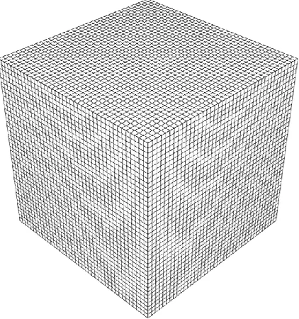
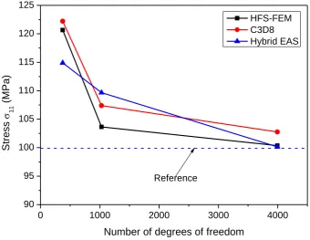
3.6.5. Cubic block under uniform tension and body force ... 59
3.6.6. Thick plate with a central hole ... 63
3.6.7. Nearly incompressible block... 66
3.7. Summary ... 68
Chapter 4. HFS-FEM for Anisotropic Composites ... 70
4.1. Introduction ... 70
4.2. Linear anisotropic elasticity ... 72
4.2.1. Basic equations and Stroh formalism ... 72
4.2.2. Foundational solutions ... 74
4.2.3. Coordinate transformation ... 75
4.3. Formulations of HFS-FEM ... 76
4.3.1. Assumed fields ... 76
4.3.2. Modified functional for HFS-FEM ... 78
xi
4.3.4. Recovery of rigid-body motion terms ... 81
4.4. Numerical examples ... 82
4.4.1. Finite orthotropic composite plate under tension ... 82
4.4.2. Orthotropic composite plate with an elliptic hole under tension ... 85
4.4.3. Cantilever composite beam under bending ... 89
4.4.4. Isotropic plate with multi-anisotropic inclusions ... 92
4.5. Summary ... 96
Chapter 5. Micromechanical Modeling of 2D Heterogeneous Composites ... 97
5.1. Introduction ... 97
5.2. Governing equations and homogenization ... 100
Governing equations of linear elasticity ... 100
Representative volume elements ... 101
Boundary conditions for RVE ... 102
Homogenization for Representative Volume Element ... 103
5.3. Formulations of the HFS-FEM ... 104
Two assumed independent fields ... 104
Modified functional for hybrid FEM ... 108
Element stiffness matrix ... 109
Recovery of rigid-body motion ... 110
5.4. Formulations of the HT-FEM ... 110
5.5. Numerical examples and discussion ... 112
Composite with isotropic fiber ... 112
5.5.1.1. Effect of mesh density ... 112
5.5.1.2. Effect of fiber volume fraction ... 116
Composites with orthotropic fibers ... 120
5.5.2.1. Effect of mesh density ... 120
5.5.2.2. Effect of fiber volume fraction ... 121
5.5.2.3. Effect of fiber shape ... 123
5.5.2.4. Effect of fiber configuration... 125
5.6. Summary ... 126
Chapter 6. Effective Thermal Conductivity of Fiber-reinforced Composites.... 128
6.2. Homogenization of heat conduction problems ... 131
Governing equations ... 131
RVE for micro-thermal analysis ... 131
Homogenization for the RVE ... 132
Boundary conditions for the RVE... 133
6.3. Fundamental solutions of plane heat conduction problems ... 134
General fundamental solution ... 135
Special fundamental solutions for hole in a plate ... 135
Special fundamental solutions for inclusion in a plate ... 137
6.4. Formulations of the HFS-FEM for heat transfer problems ... 137
Intra-element field ... 138
Auxiliary frame field... 140
Hybrid variational functional ... 140
Recovery of rigid-body motion ... 141
6.5. Numerical examples and discussion ... 142
RVE with one reinforced fiber ... 143
6.5.1.1. Convergence verification of the method ... 144
6.5.1.2. Effect of fiber volume fraction ... 145
6.5.1.3. Effect of material mismatch ratio ... 146
RVE with multiple-fibers ... 149
6.5.2.1. Effect of material mismatch ratio ... 150
6.5.2.2. Effect of fiber pattern ... 152
6.6. Summary ... 154
Chapter 7. HFS-FEM for 2D and 3D Thermo-elasticity Problems ... 155
7.1. Introduction ... 155
7.2. Basic equations for thermoelasticity ... 157
7.3. The method of particular solution ... 158
7.4. Radial basis function approximation ... 159
7.4.1. Method 1: Interpolating temperature and body force separately ... 159
7.4.2. Method 2: Interpolating temperature and body force together ... 162
7.5. Formulations of the HFS-FEM ... 163
xiii
7.5.2. Assumed fields for 3D problems... 165
7.5.3. Modified functional for HFS-FEM ... 168
7.5.4. Element stiffness matrix ... 169
7.5.5. Recovery of rigid-body motion terms ... 169
7.6. Numerical results and discussion ... 170
7.6.1. Circular cylinder with axisymmetric temperature change ... 170
7.6.2. Long beam under gravity ... 176
7.6.3. T-shaped domain with body force and temperature change .. 180
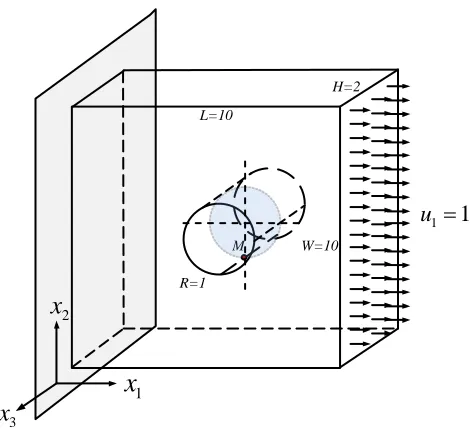
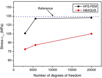
7.6.4. 3D cube under arbitrary temperature and body force ... 182
7.6.5. A heated hollow ball under varied temperature field ... 186
7.7. Summary ... 188
Chapter 8. HFS-FEM for Piezoelectric Materials ... 189
8.1. Introduction ... 189
8.2. Basic equations for piezoelectric materials ... 192
8.3. HFS-FEM based on Lekhnitskii’s formalism ... 194
8.3.1. Assumed fields ... 194
8.3.2. Variational principles ... 200
8.3.3. Element stiffness equation ... 202
8.3.4. Normalization of the variables ... 203
8.3.5. Numerical results ... 204
8.4. HFS-FEM based on Stroh Formalism ... 219
8.4.1. Extended Stroh formalism... 219
8.4.2. Foundational solutions ... 220
8.4.3. Assumed independent fields ... 224
8.4.4. Variational principles ... 226
8.4.5. Element stiffness equation ... 227
8.4.6. Numerical examples ... 228
8.5. Summary ... 238
Chapter 9. Conclusions and Outlook ... 240
9.1. Summary of present research ... 240
9.1.1. Macroscale modeling of materials by HFS-FEM ... 240
9.1.2. Microscale modeling of composites by HFS-FEM ... 241
xv
List of Tables
Table 3.1 Node coordinates and displacement boundary condition for external nodes of the 3D patch test. ... 54 Table 3.2 Comparison of normalized tip deflections of straight beam in load
direction... 56 Table 3.3 Transversal displacement and relative errors of the irregularly
meshed beam calculated by HFS-FEM and ABAQUS using
different elements. ... 59 Table 3.4 Near-incompressible regular block, displacement at the center P of
the block. ... 67 Table 4.1 Convergence of the displacement and stress at point A of the
composite plate... 84 Table 4.2 Displacement of point A of the composite plate for various fiber
orientations ... 84 Table 4.3 Deflection at the free end of the composite beam for various fiber
angles... 90 Table 4.4 Stress x along the cross section of composite beam for different
fiber angles. ... 91 Table 4.5 Comparison of displacement and stress at points A and B. ... 94 Table 5.1 Effective parameters calculated by HT-FEM and ABAQUS based
on different meshing with linear elements. ... 114 Table 5.2 Effective parameters calculated by HT-FEM, HFS-FEM and
ABAQUS using different meshing and quadratic elements. ... 114 Table 5.3 Predicted effective stiffness parameters for different FVFs using
HT-FEM with linear element ... 116 Table 5.4 Predicted effective stiffness parameters for different FVFs using
Table 5.5 Predicted effective stiffness parameters for different FVFs using
HFS-FEM. ... 119
Table 5.6 Effective stiffness parameters obtained by HFS-FEM and ABAQUS with different mesh densities ... 121
Table 5.7 Variation of effective parameters with the volume fraction of reinforced fibers ... 122
Table 5.8 Effective parameters predicted by HFS-FEM for different inclusion shapes and configuration... 125
Table 8.1 Reference values for material constants and field variables in piezoelectricity derived from basic reference variables:c0,e0,k0,0 andx0. ... 204
Table 8.2 Properties of the material PZT-4 used in Example 1 ... 205
Table 8.3 Comparison of HFS-FEM and analytical results (Sze, Yang et al. 2004) for the piezoelectric panel... 208
Table 8.4 Properties of the material PZT-4 used in Example 2 ... 210
Table 8.5 Comparison of the predicted results by HFS-FEM with the analytical results... 210
Table 8.6 Comparison of the predicted results by HFS-FEM on distorted meshes with the analytical results ... 211
Table 8.7 Mid-span predictions for bimorph under electric loading. ... 213
Table 8.8 Comparison of the SCFs obtained by HFS-FEM and ABAQUS . 215 Table 8.9 Comparison of the predicted results by HFS-FEM with the analytical results... 229
Table 8.10 Properties of the material PZT-4 used in Example 1 ... 231
Table 8.11 Properties of the material PZT-5H used in Example 4 ... 237
xvii
List of Figures
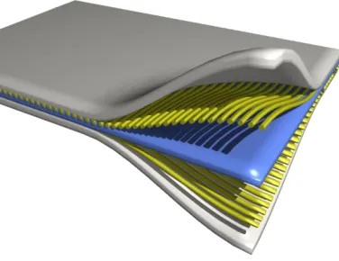
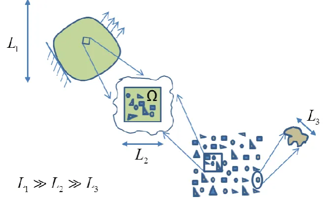
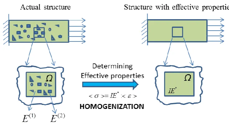
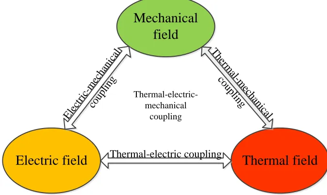
Figure 1.1 Schematic of a laminate composite plate with unidirectional ply... 3 Figure 1.2 The size requirements of a representative volume element (RVE) ... 6 Figure 1.3 Effective material properties by homogenizing the heterogeneous
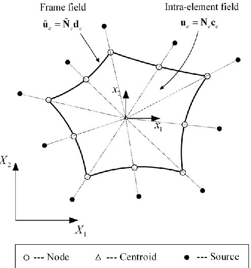
microstructure ... 7 Figure 1.4 Coupling between the three considered physical fields. ... 10 Figure 2.1 Intra-element field, frame field in a particular element in HFS-FEM,
and the generation of source points for a particular element ... 23 Figure 2.2 Typical quadratic interpolation for the frame field ... 31 Figure 2.3 Illustration of continuity between two adjacent elements ‘e’ and
‘f’ ... 32 Figure 3.1 Geometrical definitions and boundary conditions for a general 3D
solid. ... 40 Figure 3.2 Intra-element field and frame field of a hexahedron HFS-FEM
element for 3D elastic problem (The source points and centroid of 20-node element are omitted in the figure for clarity and clear view, which is similar to that of the 8-node element). ... 42 Figure 3.3 Typical linear interpolation for the frame fields. ... 44 Figure 3.4 3D patch test with wrap element (Unit cube: E =106, v = 0.25). .... 53
Figure 3.5 Perspective view of a cantilever beam under end moment:
sensitivity to mesh distortion. ... 55 Figure 3.6 Comparison of deflection at point A for a cantilever beam; (a)
deflection at point A from a cantilever beam under end moment. .. 55 Figure 3.7 Perspective views of straight cantilever beams: (a) Regular shape
Figure 3.8 Irregularly meshed bimaterial beam: geometry, materials and boundary conditions. ... 57 Figure 3.9 Irregularly meshed bimaterial beam: Mesh 1 (2×2×10 elements),
Mesh 2 (4×4×20 elements) and Mesh 3 (8×8×40 elements). ... 58 Figure 3.10 Regularly meshed bimaterial beam: fine mesh used by ABAQUS
for benchmark reference (20×20×100 elements). ... 58 Figure 3.11 Cubic block under uniform tension and body force: geometry,
boundary condition and loading... 60 Figure 3.12 Cubic block under uniform tension and body force: Mesh 1 (4×4×4
elements), Mesh 2 (6×6×6 elements) and Mesh 3 (10×10×10
elements). ... 60 Figure 3.13 Cubic block under uniform tension and body force: fine mesh used
by ABAQUS for benchmark reference (40×40×40 elements). ... 61 Figure 3.14 Cubic block with body force under uniform distributed load:
Convergent study of displacements. ... 61 Figure 3.15 Cubic block with body force under uniform distributed load:
Convergent study of stresses. ... 62 Figure 3.16 Contour plots of displacement u1 and stress 11 of the cube. ... 62
Figure 3.17 Thick plate with central hole: geometry, material and boundary conditions. ... 64 Figure 3.18 Thick plate with central hole: fine mesh used by ABAQUS for
benchmark reference (138866 elements with 151725 nodes). ... 64 Figure 3.19 Perforated thick plate: Mesh 1 (660 elements with 985 nodes), Mesh
2 (1392 elements with 1876 nodes) and Mesh 3 (5274 elements with 6657 nodes). ... 65 Figure 3.20 Perforated thick plate under uniform distributed load: Convergent
xix
Figure 3.21 Perforated thick plate under uniform distributed load: Convergent study of Von Mises stress. ... 66 Figure 3.22 Nearly incompressible block: geometry, boundary conditions and
the tested mesh (1/4 model). ... 67 Figure 3.23 Contour plot of the vertical displacements of the
near-incompressible regular block under central uniform loading. ... 68 Figure 4.1 Schematic of a composite laminate. ... 70 Figure 4.2 Schematic of the relationship between global coordinate system and local material coordinate system (1, 2). ... 75 Figure 4.3 Schematic of an orthotropic composite plate under tension. ... 83 Figure 4.4 Two mesh configurations (left: 4×4 elements, right: 10×10
elements) for the orthotropic composite plate. ... 83 Figure 4.5 Variation of the displacements at point A of orthotropic plate with
fiber orientation. ... 84 Figure 4.6 Schematic of an orthotropic composite plate with an elliptic hole
under uniform tension. ... 85 Figure 4.7 Mesh configurations for the orthotropic composite plate with an
elliptic hole: (a) for HFS-FEM; (b) for ABAQUS ... 86 Figure 4.8 Variation of hoop stresses along the rim of the elliptical hole for
different fiber orientation . ... 86 Figure 4.9 Contour plots of stress components around the elliptic hole in the
composite plate... 88 Figure 4.10 Variation of SCF with the lamina angle . ... 89 Figure 4.11 Schematic of a cantilever composite beam under bending. ... 89 Figure 4.12 Schematic of an isotropic plate with multi-anisotropic inclusions. 93 Figure 4.13 Mesh configuration of an isotropic plate with multi-anisotropic
Figure 4.14 The variation of displacement component u1 along the right edge of
the plate (x=8) by HFS-FEM and ABAQUS. ... 95 Figure 4.15 The variation of displacement component u2 along the right edge of
the plate (x=8) by HFS-FEM and ABAQUS. ... 95 Figure 4.16 Contour plots of displacement u1, u2 and stress 11 for the
composite plate. ... 96 Figure 5.1 Schematic of representative volume elements (RVE) ... 101 Figure 5.2 Schematic of periodic boundary conditions of RVE ... 103 Figure 5.3 Intra-element field and frame field in a particular element of a
HFS-FEM element for plane elastic problems ... 105 Figure 5.4 Intra-element field and frame field of a HT-FEM element for plane
elastic problems ... 108 Figure 5.5 Three different mesh densities (Red: Fiber, Yellow: Matrix)... 113 Figure 5.6 Stress fields of the RVE of composites with isotropic fiber on
deformed configuration under pure shear strain using (a) HT-FEM and (b) HFS-FEM (FVF: 28.27%). ... 116 Figure 5.7 Variation of the composite effective parameters with increasing
FVF using HT-FEM (Linear and quadratic elements). ... 117 Figure 5.8 Variation of the Young’s elastic modules ETof composite with
increasing FVF using HT-FEM. ... 118 Figure 5.9 Variation of Poison’s ration vTof the composite with increasing
FVF using HT-FEM. ... 119 Figure 5.10 Comparison of effective stiffness parameters calculated by
HFS-FEM and ABAQUS. ... 121 Figure 5.11 Mesh, deformation and stress fields of the RVE of composites with
xxi
Figure 5.12 Variation of effective parameters with increasing FVF ... 124
Figure 5.13 Meshes for RVE with different-shaped fibers ... 124
Figure 5.14 Meshes for RVE with different fiber configurations ... 125
Figure 5.15 Difference of effective parameters among six configurations ... 126
Figure 6.1 Periodic fiber-reinforce composites and RVE. ... 132
Figure 6.2 Schematic for the definition of general fundamental solutions of plane heat conduction problems. ... 135
Figure 6.3 Schematic for the definition of special fundamental solutions (hole) of plane heat conduction problems. ... 136
Figure 6.4 Schematic for the definition of special fundamental solutions (inclusion) of plane heat conduction in fiber-reinforced composites. ... 137
Figure 6.5 Intra-element field, frame field in a special element of HFS-FEM, and the generation of its source points ... 139
Figure 6.6 Schematic of RVE containing one central fiber ... 143
Figure 6.7 Mesh configurations for RVE by (a) HFS-FEM with special element (White: matrix, Green: fiber) and by (b) ABAQUS. ... 144
Figure 6.8 RVE with one central fiber: Convergence of the effective thermal conductivity. ... 145
Figure 6.9 Effective thermal conductivities k of composite for different fiber volume factions. ... 146
Figure 6.10 Effective thermal conductivity k* of the composite for different mismatch ratios when k2>k1 ... 147
Figure 6.11 Effective thermal conductivity k* of the composite for different mismatch ratios when k1>k2. ... 148
Figure 6.13 Contour plots of the temperature and heat flux distribution in the RVE (1/m=20, FVF=19.63%) ... 149 Figure 6.14 RVEs of the composite with two different fiber configurations ... 149 Figure 6.15 Mesh configurations of the RVEs for HFS-FEM. ... 150 Figure 6.16 Mesh configurations of the RVEs for ABAQUS. ... 150 Figure 6.17 Effective thermal conductivity k* of the composite for different
mismatch ratios when k2>k1 ... 151
Figure 6.18 Effective thermal conductivity k* of the composite for different
mismatch ratios when k1>k2. ... 152
Figure 6.19 Contour plots of the temperature and heat flux distribution in the RVE (m=20, FVF=15.71%) ... 153 Figure 6.20 Contour plots of the temperature and heat flux distribution in the
RVE (1/m=20, FVF=15.71%) ... 153 Figure 7.1 Geometrical definitions and boundary conditions for general 3D
problems ... 158 Figure 7.2 Intra-element field and frame field of a HFS-FEM element for 2D
thermoelastic problems ... 164 Figure 7.3 Intra-element field and frame field of a hexahedron HFS-FEM
element for 3D thermoelastic problem (The source points and centroid of 20-node element are omitted in the figure for clarity and clear view, which is similar to that of the 8-node element) ... 166 Figure 7.4 Typical quadratic interpolation for the frame fields ... 168 Figure 7.5 Geometry and boundary conditions of the long cylinder with
axisymmetric temperature change. ... 171 Figure 7.6 Mesh configurations of a quarter of circular cylinder: (a) Coarse
Mesh (Left: 16 elements) and (b) Fine Mesh (Right: 128
xxiii
Figure 7.7 Variation of the radial thermal stresses with the cylinder radius using coarse mesh (a) and fine mesh (b) ... 173 Figure 7.8 Variation of the circumferential thermal stresses with the cylinder
radius using (a) coarse mesh and (b) fine mesh ... 174 Figure 7.9 Variation of the radial displacement with the cylinder radius using
(a) coarse mesh and (b) fine mesh... 175 Figure 7.10 Contour plots of (a) radial and (b) circumferential thermal stresses
(The meshes used for contour plot is different from that for
calculation due to using quadratic elements) ... 176 Figure 7.11 Long square cross-section beam under gravity ... 177 Figure 7.12 Mesh configuration of square cross-section beam ... 177 Figure 7.13 Displacement and stresses along x1=10 of square cross-section of
the beam ... 179 Figure 7.14 Contour plots of the stresses of square cross-section beam ... 179 Figure 7.15 Dimension and boundary condition of the T-Shape domain ... 180 Figure 7.16 Mesh configuration of T-Shape domain ... 180 Figure 7.17 The variation of the thermal stresses of T-Shape domain: (a) 11
along line x2 14 and (b) 22 along line x10... 182 Figure 7.18 Contour plots of the displacement and stresses of T-Shape domain
under temperature change and body force ... 183 Figure 7.19 Schematic of the cube under arbitrary temperature and body
force... 184 Figure 7.20 Mesh configurations of the 3D cube under arbitrary temperature and
body force... 184 Figure 7.21 Displacement u3 and stress 33 along one cube edge when
Figure 7.23 Mesh configurations of the heated hollow ball: (a) for HFS-FEM and (b) for ABAQUS ... 186 Figure 7.24 Radial displacement and Von Mises stress along radius of the
heated hollow ball subjected to temperature change ... 188 Figure 8.1 Intra-element field and frame field of HFS-FEM element for 2D
piezoelectric problem: general element (left) and special element with central elliptical hole (right). ... 194 Figure 8.2 Illustration of continuity between two adjacent elements ‘e’ and
‘f’ ... 201 Figure 8.3 Bending of a piezoelectric panel ... 206 Figure 8.4 Mesh used for the piezoelectric panel by HFS-FEM ... 206 Figure 8.5 variation of the stress xx at point A (0, 0.5mm) with parameter
... 207 Figure 8.6 Variation of the condition number of H matrix and K matrix with
parameter ... 207 Figure 8.7 Contour plots of displacements, electrical potential and stress .... 208 Figure 8.8 Geometry and boundary conditions of the piezoelectric prism .... 209 Figure 8.9 Regular (Left) and distorted (Right) meshes used for modeling the
piezoelectric prism ... 210 Figure 8.10 Contour plot of the displacements and electric potential of the
plate ... 211 Figure 8.11 A simply supported bimorph piezoelectric beam (x z : local
material coordinate system). ... 212 Figure 8.12 Element Mesh used for modeling the bimorph piezoelectric beam in HFS-FEM analysis ... 212 Figure 8.13 An infinite piezoelectric plate with a circular hole subjected to
xxv
Figure 8.14 Element meshes used for HFS-FEM (left) and ABAQUS (right) in the case of L/r=20 ... 214 Figure 8.15 Distribution of (a) hoop stress and (b) radial stress r along the
line z=0 when subjected to remote mechanical load xx and along the line x=0 when subjected to remote mechanical load zz. ... 217 Figure 8.16 Variation of normalized stress / 0 along the hole boundary
under remote mechanical loading ... 218 Figure 8.17 Variation of normalized electrical displacement 10
0 / 10
D along
the hole boundary under remote mechanical loading ... 218 Figure 8.18 Schematic of the infinite anisotropic plate with an elliptical hole .. 222 Figure 8.19 Conformal mapping of an infinite plane with an elliptical hole ... 222 Figure 8.20 Geometry, boundary conditions and mesh configuration of the
piezoelectric prism ... 229 Figure 8.21 Contour plot of the displacement and electric potential of the
plate ... 230 Figure 8.22 An infinite piezoelectric plate with a circular hole subjected to
remote stress ... 231 Figure 8.23 Variation of normalized stress / 0 along the hole boundary
under remote mechanical load ... 232 Figure 8.24 Variation of normalized electrical displacement 10
0 / 10
D along
the hole boundary under remote mechanical load... 232 Figure 8.25 Variation of normalized stress 8
0 /D 10
along the hole boundary under remote electrical load ... 233 Figure 8.26 Variation of normalized electrical displacement D /D0along the
Figure 8.27 Contour plots of stress and electric displacement components around the elliptic hole in the piezoelectric plate under remote mechanical load. ... 234 Figure 8.28 Schematic of an infinite piezoelectric plate with an elliptic hole
under remote tension. ... 235 Figure 8.29 Mesh configuration with special element for the piezoelectric
plate ... 235 Figure 8.30 Contour plots of stress components around the elliptic hole in the
composite plate. ... 236 Figure 8.32 The variation of KIVwith respect to the applied remote electric
displacement Dzz ... 238
Chapter 1.
Introduction
1.1.BACKGROUND AND MOTIVATION
Advanced composite materials are being increasingly used in a variety of fields such as aerospace, automobile, defense, medical and sports due to their preferred mechanical behaviors and desired properties. Examples of their desirable properties are light weight, high stiffness or high flexibility, good thermal and mechanical durability, high yield strength under static or dynamic loading and good surface hardness. Some smart structures can energy transform among different forms such as piezoelectric sensors. Many of these materials, either human-designed or natural, are heterogeneous and have complex microstructures at a certain scale, features that increases the challenges involved in product design and analysis. The heterogeneous microstructure of composites has a significant impact on their observed macroscopic behavior. Indeed, the overall behavior of these materials depends strongly on the size, shape, spatial distribution and properties of the microstructural constituents and their respective interfaces (Wriggers and Hain 2007).
The main motivation of this research is to develop a new efficient methodology for modeling advanced composite materials and to assess the performance of the method in predicting behaviors of these materials at both micro and macro scales. The research also underscores the need for convenient performance of multiphysics analyses and for thorough understanding of the underlying mechanisms. The work presented lays the foundation for establishing a multiscale framework to facilitate the design and analysis of advanced materials such as the carbon nanotube reinforced composites and piezoelectric materials widely used in smart structures and materials.
1.2.MODELING OF ADVANCED MATERIALS
With the advances in computing power and simulation methodology, computational modeling has been increasingly employed in the design and development of advanced composites. During the past several decades, a few methods have been proposed and successfully applied to modeling composites from nanoscale to macroscale (Ghosh, Nowak et al. 1997; Yang and Qin 2003; Chawla, Ganesh et al. 2004; Yang and Qin 2004; Ghosh, Bai et al. 2009). In the following section of the chapter, a brief literature review on the modeling of composites is presented from the perspectives of macro-, micro- and multi-scale.
1.2.1.Macroscale modeling of composites
Composite materials were first used in aircraft engine rotor blades in the 1960s. Since then, a great deal of research has been conducted to improve the properties of composite materials; now numerous publications cover anisotropic elasticity, mechanics of composite materials, design, analysis, fabrication, and application of composite structures (Lekhnitskii 1968; Lekhnitskii 1981; Reddy 2004; Vasiliev and Morozov 2007).
their stacking sequence, geometric and mechanical properties (Vasiliev and Morozov 2007).
Figure 1.1 Schematic of a laminate composite plate with unidirectional ply.
Extensive research has been performed on damage modeling of composites and a number of models have been proposed to predict damage accumulation (Shokrieh and Lessard 2000; Dvorak and Zhang 2001; Van Paepegem and Degrieck 2003). Among those, progressive damage models that use one or more damage variables related to measurable manifestations of damage (interface debonding, transverse matrix cracks, delamination size, etc.) are considered the most promising because they quantitatively account for the accumulation of damage in the composite structure. Kumar et al. studied the effect of impactor and laminate parameters on the impact response and impact-induced damages in graphite/epoxy laminated cylindrical shells using three-dimensional (3D) finite element formulation (Kumar, Rao et al. 2007). Ghosh and Sinha (2004) developed a finite element analysis procedure to predict the initiation and propagation of damages as well as to analyze laminated composite plates damaged under forced vibration and impact loads. Zhao and Cho (2004) investigated the impact-induced damage initiation and propagation in the laminated composite shell under low-velocity impact. In addition, Abrate (1994) presented an overview of the work carried out by different researchers in the field of the optimum design of composite laminated plates and shells subjected to constraints on strength, stiffness, buckling loads and fundamental natural frequencies.
1.2.2.Microscale modeling of composites
properties of the composites, but also various mechanisms such as damage initiation, crack growth and propagation can also be studied through microscale analysis.
In micromechanical analysis, the macroscopic properties are determined by a homogenization process that yields the effective stresses and strains acting on an effective, homogenized sample of material. Not long ago, homogenization and the determination of effective material parameters could only be done either by performing experiments or tests with an existing material sample or by applying semi-analytical methods with strong assumptions on the mechanical field variables or the microstructure of the material. There are several analytical micromechanical techniques extensively employed in practice such as the Eshelby approach, Mori-Tanaka method and Halpin-Tsai method (Eshelby 1957; Hill 1963; Mori and Mori-Tanaka 1973; Hashin 1983; Benveniste 1987; Aboudi 1991; Nemat-Nasser and Hori 1999). However, these semi-analytical methods do not lead to sufficiently accurate results, especially for complex morphologies, high contrast in phase properties material nonlinearities and more non-proportional load histories. This suggests the need to carry out direct numerical simulation of microstructures and to try to establish a realistic representation of the heterogeneous structure that appends and contains all the microscale details.
interior fields inside the domain; additionally, for solving multi-domain problems with BEM, each region is dealt with separately and then the whole body is linked together by applying compatibility and equilibrium conditions along the interfaces between the subregions. In consequence, implementation of the BEM becomes quite complex and the nonsymmetrical coefficient matrix of the resulting equations weakens the advantages of BEM (Qin 2000; Qin 2004). Nowadays sophisticated and efficient models to simulate realistic material behaviors continue to be developed in this active research area.
Figure 1.2 The size requirements of a representative volume element (RVE).
The interface damage between fiber and matrix is also studied explicitly in the framework of a RVE of the composite (Caporale, Luciano et al. 2006; Aghdam, Falahatgar et al. 2008; Maligno, Warrior et al. 2009; Kushch, Shmegera et al. 2011). A RVE combined with proper boundary conditions to represent as closely as possible the real composite material macro-behavior would provide a tool to enhance practical understanding of the composite’s material behavior based on its micro-constituents.
Figure 1.3 Effective material properties by homogenizing the heterogeneous microstructure.
1.2.3.Multiscale modeling of composites
In the so-called multiscale modeling, macroscopic and microscopic models are coupled to take advantage of the efficiency of macroscopic models and the accuracy of the microscopic models. Multiscale modeling involves the design of combined macroscopic-microscopic computational methods that are more efficient than solving the full microscopic model and at the same time provides needed the information with desired accuracy. The asymptotic homogenization method is based on asymptotic expansion of the displacement, strain and stress fields and assumptions of spatial periodicity of microscopic RVEs (Bensoussan, Lions et al. 1978; Sánchez-Palencia 1980). Concurrent multiscale analyses are executed at macro- and micro-scales with information transfer between them (Fish, Yu et al. 1999; Kouznetsova, Brekelmans et al. 2001; Terada and Kikuchi 2001; Özdemir, Brekelmans et al. 2008; Yuan and Fish 2009). Ghosh and co-workers (Ghosh, Lee et al. 2001) combined the asymptotic homogenization method with the micro-mechanical Voronoi cell finite element method for multiscale analysis of deformation and damage in non-uniformly distributed microstructures.
1.2.4.Modeling of multifield materials
Multifield materials have attracted much attention from researchers and scientists for their capability of interactively transferring energy from one type to another (Parton and Kudryavtsev 1988). These “smart materials” are responsive to multiphysical fields such as electric, magnetic or thermal fields in addition to the traditional mechanical field. Examples include piezoelectric ceramics, piezoelectric polymers and some biological tissues like bones. Piezoelectric materials are the most popular smart materials: they undergo deformation (strain) when an electric field is applied across them, and conversely produce voltage when a strain is applied, and thus can be used both as actuators and sensors. The coupling behaviors of these multifield materials are critical and unique for their applications in adaptive structures, actuators and sensors. It is of paramount important, therefore, to investigate the coupling behaviors of these materials for product design and analysis.
Meric and Saigal (1990) derived shape sensitivity expressions for linear piezoelectric structures with coupled mechanical and elastic field. Suleman and Venkayya (1995) presented a simple finite element formulation for laminated composite plates with piezoelectric layers. Chattopadhyay and Seeley (1997) used a finite element model based on a refined higher order theory to analyze piezoelectric materials surface bonded or embedded in composite laminates. Varelis and Saravanos (2008) presented a coupled multi-field mechanics framework for analyzing the non-linear response of shallow doubly curved adaptive laminated piezoelectric shells undergoing large displacements and rotations in thermal environments.
piezoelectricity and succeeded in applying them to establish a Trefftz finite element formulation. Jin et al (2005) formulated the Trefftz collocation and the Trefftz Galerkin methods for plane piezoelectricity based on the solution sets derived by the complex variables method. Sheng et al (2006) developed a multi-domain Trefftz boundary collocation method for plane piezoelectricity with defects according to the plane piezoelectricity solution derived by Lekhnitskii’s formalism. In addition, much work has been done on micromechanics modeling for designing a smart composite, e.g. piezoelectric composites, shape memory alloy (SMA) fiber composites, and piezoresistive composites, where smart materials with coupling behavior are used as reinforcement (Minoru 1999).
Figure 1.4 Coupling between the three considered physical fields.
In the present dissertation three physical fields are considered: mechanical, electrical and thermal field and their possible interactions (see Figure 1.4). The possible interactions are:
One field problem: mechanical problem, thermal problem, electrical problem.
Two fields problem: thermo-mechanical coupling, electro-mechanical coupling, and thermo-electrical coupling;
Mechanical
field
Thermal field
Electric field
Thermal-electric couplingEle ctri
c-m echa
nica l
coup ling
T herm
al-m echa
nic al co
up ling
Thermal-electric-mechanical
Three fields problem: electro-thermo-mechanical coupling;
1.3.HYBRID FINITE ELEMENT METHOD
1.3.1.Hybrid Trefftz finite element method
The HT-FEM can be regarded as a variant of the conventional formulations of the FEM (Ritz-method-based FEM). The concept of Trefftz consists simply of using an approximation basis extracted from the solution set of the governing system of differential equations. When this concept is implemented in the framework of the FEM released from both node and local conformity concepts, the resulting finite element solving systems are sparse, free of spurious modes, and well-suited to adaptive refinement and parallel processing (Qin 2000; Toma 2007).
As Trefftz bases embody the physics of the problem, substantially higher levels of performance are observed in accuracy, stability and convergence (Jirousek and Wroblewski 1996; Qin 2000). Moreover, this basis leads to a solving system in which all coefficients are defined by boundary integral expressions. Hence, it leads to a formulation that combines the main features of the FEM and BEM, namely domain decomposition and boundary integral expressions, while dispensing with the use of (strongly singular) fundamental solutions and avoiding the major weaknesses of BEM, such as singularity and loss of symmetry and sparsity (Toma 2007).
This approach involves only element boundary integrals, inherits the advantages of both conventional FEM and BEM, and has been successfully applied to various engineering problems (Qin 1994; Qin 1995; Qin 1996; Qin 2003; Qin and Wang 2008). The main advantages of HTFEM are: (a) it is only integral along element boundaries, enabling arbitrary polygonal or even curve-sided elements to be used; (b) no singular element boundary integral is involved; (c) it is likely to represent the optimal expansion bases for hybrid-type elements where inter-element continuity need not to be satisfied; (d) it can develop accurate crack-tip, singular corner or perforated elements by using appropriate known local solution functions as the trial functions of intra-element displacements (Qin 2003). However, the terms of truncated T-complete functions must be carefully selected to achieve the desired results, and it is difficult to generate T-complete functions for certain complex or new physical problems (Qin 2000; Qin and Wang 2008). Further, in the HT-FEM a coordinate transformation is required to keep the system matrix stable, and the necessary variational functional is somewhat complex for practical use.
The earliest applications of general purpose Trefftz elements can be dated back to 1977 when Jiroušek presented four formulations for solid mechanics problems (Jirousek and Leon 1977; Jirousek 1978), in which nonconforming elements are assumed to fulfill the governing equations a priori and the inter-element continuity and the boundary conditions are then enforced in some weighted residual or point-wise sense. Later Herrera (1980) introduced completeness and convergence criteria and Cheung et al. (Cheung, Jin et al. 1989; Jin and Cheung 1995) proposed the direct Trefftz boundary element method in opposition to the so-called indirect approach of Jiroušek by enforcing in a weak form of the governing differential equation, using a complete basis as weighting functions.
(Jirousek, Wroblewski et al. 1995; Jirousek, Wróblewski et al. 1995), thick plates (Piltner 1992), thin shells (Voros 1991), general 3-D solid mechanics (Piltner 1987; Piltner 1992; de Freitas and Bussamra 2000), the Poisson equation (Zielinski and Zienkiewicz 1985), transient heat conduction analysis (Jirousek and Qin 1995), nonlinear problems (Qin 1996; Qin and Diao 1996; Qin 2005), and piezoelectric problems (Qin 2003; Qin 2003). Moreover, the h-version and the p-version of T-elements have been suggested, implemented and studied (Jirousek 1987; Jirousek and Venkatesh 1989; Qin and Diao 1996). Besides, special-purpose elements have been proposed to deal with various geometries or load-dependent singularities and local defects such as obtuse corners, cracks, holes, and concentrated load (Piltner 1985; Jirousek and Guex 1986; Dhanasekar, Han et al. 2006).
1.3.2.Hybrid fundamental solution-based finite element method
Based on the framework of HT-FEM and the idea of the method of fundamental solution (MFS), a novel hybrid finite element formulation, called the Hybrid fundamental solution-based FEM (HFS-FEM), was recently developed for solving 2D linear heat conduction problems (Wang and Qin 2009; Wang and Qin 2010a), elastic problems (Wang and Qin 2010b; Cao, Qin et al. 2012a; Cao, Qin et al. 2013a), and piezoelectric problems (Cao, Qin et al. 2012b; Cao, Yu et al. 2013c). In HFS-FEM, fundamental solutions rather than T-complete functions are employed, which also exactly satisfy a priori the governing equations for the problem under consideration. In the approach, the intra-element field is approximated by the linear combination of the fundamental solutions analytically satisfying the related governing equation, and the domain integrals in the hybrid functional can be directly converted to boundary integrals without any appreciable increase in computational effort. It is also noticed that no singular integrals are involved in the HFS-FEM if the source point is located outside the element of interest and does not overlap with field point during computation (Wang and Qin 2010a). The resulting system of equations from the modified hybrid variational functional is expressed in terms of symmetric stiffness matrix and nodal displacements only, which is easy to implement into the standard FEM.
It should be noted that, however, the HFS-FEM approach differs from the BEM, although the same fundamental solution is employed. Using the reciprocal theorem, the BEM obtains the boundary integral equation, and usually encounters difficulty in dealing with singular or hyper-singular integrals in the analysis, while this weakness is removed using HFS-FEM. Moreover, HFS-FEM makes possible a more flexible element material definition which is important in dealing with multi-material problems, rather than the material definition being the same in the entire domain in BEM.
1.4.OBJECTIVES OF RESEARCH
HFS-FEM has been proposed for solving 2D elasticity and heat transfer problems. Considering the attractive merits of this method, it is of interest to further extend this method for wider applications in the modeling of advanced materials across micro and macro scales. Thus, the main objectives of this research can be defined as follows:
To develop formulations of the method for both the 2D and 3D elasticity problems;
To formulate an alternative formulations based on the Stroh formalism for modeling anisotropic composites and to assess its performance in simulation;
To develop and assess the HFS-FEM in micromechanical modeling of heterogeneous composite materials based on the homogenization method and RVE concept, for both elasticity problem and heat conduction problem;
To assess the performance of the elements used in HFS-FEM in terms of convergence and of their sensitivity to mesh distortion and materials incompressibility;
To develop HFS-FEM formulations for modeling multifield materials such as thermal-mechanical and electric-mechanical problems.
1.5.SCOPE AND ORGANIZATION OF THESIS
The dissertation is organized in three main parts (i.e. macroscale modeling of elasticity and composites, microscale modeling of composites, and modeling of multifield problems) divided into nine chapters. In Chapter 1, the background and motivation of this research are firstly introduced, followed by a brief literature review of the topics discussed in this thesis. The research objectives are also stated. In Chapter 2, the basic ideas and the detailed formulations of the HFS-FEM for elasticity and potential problems are presented based on relevant previous research.
Chapter 3 proposes the formulations of the HFS-FEM for general 3D elasticity problems. The methods of particular solution and radial basis function approximation are proposed to deal with body force. Standard tests are carried out for a linear 8-node brick element and quadratic 20-node brick element. Several numerical examples are performed to investigate the method for modeling various problems including nearly incompressible materials.
Chapter 4 proposes a new formulation of HFS-FEM for 2D anisotropic composite materials based on the powerful Stroh formalism. The Stroh formalism and the derived fundamental solutions for generalized 2D anisotropic elastic problem are presented. Four numerical examples are presented to demonstrate the accuracy and efficiency of the proposed method.
homogenization method and representative volume element (RVE) concepts are introduced in this context. For comparison, formulations of the HT-FEM are also presented in this chapter. The effect of fiber volume fractions, different inclusion shapes and arrangements on the effective stiffness coefficients of composites are investigated using the proposed micromechanical models.
Chapter 6 has basically the same structure as Chapter 5. In Chapter 6, formulations of the HFS-FEM for heat conduction problem are presented to model heterogeneous fiber-reinforced composites. Both the general element and special elements for circular hole and inclusion are proposed based on the relevant fundamental solutions to reduce the mesh refinement effort in modeling heterogeneous composites. A homogenization procedure for non-mechanical field variables is introduced for estimating the effective thermal properties of composites. Two examples are considered to assess the performance of the method and to investigate the influence of fiber volume fraction and fiber arrangement pattern on the effective thermal conductivity.
Chapter 7 extends the HFS-FEM to model 2D and 3D thermoelastic problems considering arbitrary body forces and temperature change. The method of particular solution is used to decompose the displacement solution into two parts: homogeneous solution and particular solution. The particular solution related to the body force and temperature change is approximated by using the radial basis function interpolation. Five different numerical examples are presented to demonstrate the accuracy and versatility of the proposed method.
derive the element stiffness matrix of the proposed method for piezoelectric materials. Numerical examples are presented to assess the accuracy and efficiency of the proposed formulations.
Chapter 2.
Framework of HFS-FEM for Plane Elasticity and
Potential Problems
2.1.INTRODUCTION
During past decades, research into the development of efficient finite elements has mostly concentrated on the three variants of FEM. The first is the conventional (Ritz based) FEM (Zienkiewicz, Taylor et al. 2005), which is based on polynomial interpolations and has been increasingly used for analyzing most engineering problems. With this method, the domain of interest is divided into a number of smaller sub-domains or elements, and material properties are defined at the element level. The second variant, the natural-mode FEM (Argyris, Dunne et al. 1974), presents a significant alternative to conventional FEM with ramifications on all aspects of structural analysis. It makes a distinction between the constitutive and geometric parts of the element tangent stiffness, which can lead effortlessly to the non-linear effects associated with large displacements. When applied to composite structures, the physically clear and comprehensible theory with complete quadrature elimination and avoidance of modal (shape) functions can show distinctly the mechanical behavior of isotropic and composite shell structures (Tenek and Argyris 1997).
The third variant is the so-called HT-FEM (Qin 1995; Jirousek and Wroblewski 1996; Qin 2000). Unlike the other two methods, HT-FEM is based on a hybrid method that combines two independent assumed fields, an auxiliary inter-element frame field defined on each inter-element boundary and an intra-inter-element field chosen so as to a priori satisfy the homogeneous governing differential equations. Inter-element continuity is enforced by using a modified variational principle, which is used to construct the standard force-displacement relationship. The HT-FEM combines the advantages of FEM and BEM, as addressed in Chapter 1.
some physical problems. To eliminate this drawback of HT-FEM, a novel hybrid finite formulation based on fundamental solutions, HFS-FEM, was first developed to solve 2D heat conduction problems in single and multilayer-materials (Wang and Qin 2009). It was then developed and successfully applied to analyze plane elasticity problems under various loading conditions (Wang and Qin 2010b). The proposed HFS-FEM can be viewed as another variant of hybrid FEM which is different from the three aforementioned types. Sophisticated and efficient models for simulating realistic material behaviors still continue to be developed in this active research area.
In this chapter, the framework of the HFS-FEM for 2D elasticity and potential problems is presented in detail, with the intention of providing a general overview of the recently proposed method. The detailed procedures and implementation of the HFS-FEM are all described. The two independent fields assumed in this method are highlighted, and the modified variaitional function to assure the continuity between elements is addressed and proved. The numerical integral and its implementation are given and the rigid motion recovery is also presented for complementation. In summary, this can be regarded as a brief review of the relevant work by some members of the candidate’s research group over the past three years. It also serves as the foundation of this dissertation which presents further development and application of this new method for modeling advanced composite materials, and is also a reference for the following chapters. Most of the materials presented in this chapter are organized and extended based on previous papers (Wang and Qin 2009; Wang and Qin 2010a; Wang and Qin 2010b) and a book (Qin and Wang 2008) published by Q.H. Qin and his co-worker.
2.2.FORMULATIONS OF HFS-FEM FOR ELASTICITY
2.2.1.Linear theory of plane elasticity
1970). In the rectangular Cartesian coordinates (X1, X2), the governing equations of
plane elasticity can be expressed as
, , , 1, 2 ij j bi i j
(2.1)
If written in matrix form, it can be presented as
Lσ b (2.2)
where the stress vector
T 11 22 12
σ , the body force vector
T1, 2
b b
b and the
differential operator matrix L is given as
1 2 2 1 0 0 X X X X L (2.3)
The strain-displacement relation is expressed in matrix form as
T
ε = L u (2.4)
where the strain vector ε
11 22 12
T, and the displacement vector u
u u1, 2
T. The constitutive equations for linear elasticity are given in matrix form as
σ Dε (2.5)
where D is the material coefficient matrix with constant components for isotropic
materials, which can be expressed as follows
0 0 2 0 2 0 G G G D (2.6) where
2 ,1 2 2 1
E G G
(2.7)
and
for plane strain for plane stress 1 v (2.8)
where E is Young’s module and v Poisson’s ratio. The two different kinds of boundary conditions can be expressed as
on on u t u u
where t[t1 t2]T denotes the traction vector, u are the prescribed boundary
displacement vector and t the prescribed traction vector, and Ais a transformation
matrix related to the direction cosine of the outward normal
1 2 2 1 0 0 n n n n A (2.10)
where ni is the unit outward normal to the boundary. Substituting Eqs. (2.4) and (2.5)
into Eq. (2.2) yields the well-known Navier partial differential equations in terms of displacements
T
LDL u b (2.11)
2.2.2.Assumed fields
The main concept of the HFS-FEM approach is to establish a finite element formulation whereby intra-element continuity is enforced on a nonconforming internal displacement field by a functional (Wang and Qin 2010a). In this approach, the intra-element displacement fields are approximated by a linear combination of fundamental solutions of the problem of interest, as follows;
11 12 1
1
1 12 22 2
2 ( , ) ( , ) ( ) ( , ) ( , ) ( ) s n
sj sj j
j sj sj j
u u c
u
u u c
u
e ex y x y
x
u(x) N c
x y x y
x (2.12)
where ns is the number of source points ysj(j1, 2, ,ns) arranged outside the element to remove the singularity of the fundamental solution. In the analysis, the number of source points can be taken to be the same as the number of element nodes, which is free of spurious energy modes and can maintain the stiffness equations in full rank, as indicated in (Qin 2000). The matrix Ne and vector cecan be written as
11 1 12 1 11 12
12 1 22 1 12 22
( , ) ( , ) ... ( , ) ( , ) ( , ) ( , ) ... ( , ) ( , )
s s
s s
s s sn sn
s s sn sn
u u u u
u u u u
e
x y x y x y x y
N
x y x y x y x y (2.13)
11 21 1 2
[c c ... cn c n]T
e
c (2.14)
11
1 2
21 12
2 2 2
2 1
2
2
2 2
[(3 4 ) ln ]
[(3 4 ) ln ] ( , )
( , ) ( , ) ( , )
u A r
r r r
u u A
r r u
r
A r
r
s
s s
s x y
x y x x
x y
(2.15)
where ri xi xis ,r r12r22 , A 1/ 8G(1) for isotropic materials (Sauter
[image:49.595.197.445.230.495.2]and Schwab 2010 ).
Figure 2.1 Intra-element field, frame field in a particular element in HFS-FEM, and the generation of source points for a particular element.
The source point xsj(j1, 2, ,ns)can be generated by means of the following method employed in the MFS (Wang, Qin et al. 2006; Hui and Qinghua 2007; Wang and Qin 2010a)
b b c
y x x x (2.16)
simplicity. Determination of must be discussed for different problems (Wang and
Qin 2009; Wang and Qin 2010b).
Making use of the constitutive Eq. (2.5), the corresponding stress fields can be expressed as
e e
σ(x) T c (2.17)
where
111 1 211 1 111 211
122 1 222 1 122 222
112 1 212 1 112 212
( , ) ( , ) ... ( , ) ( , ) ( , ) ( , ) ... ( , ) ( , ) ( , ) ( , ) ... ( , ) ( , ) s s s s s s n n n n n n e
x y x y x y x y
T x y x y x y x y
x y x y x y x y
(2.18)
As a consequence, the traction is written as 1 2 t t
e e
t nσ Q c (2.19)
in which
e e
Q nT , 1 2
2 1 0 0 n n n n n (2.20)
The corresponding stress components ijk( , )x y are expressed as
4 2 4 2
4
3 2
1 1 1 2 1
111 11 12
3 2
1 1 1 2 1
221 12 22
2
1 2 2
12
2 4 2
4 2
1 66
2 (1 4 ) 2
( ) ( )
2 (1 4 ) 2
( ) ( )
4 2(1 2 )
( )
r r r r r
Ac Ac
r r r r
r r r r r
Ac Ac
r r r r
r r r
c r A r (2.21) 2 3
1 2 2 2 2
112 11 12
2 3
1 2 2 2 2
222 12 22
2 1 1 2 122
4 2 2 4
4 2 4
4 6
2
2 6
2 (1 4 ) 2
{ ( ) ( )}
2 (1 4 ) 2
{ ( ) ( )}
2(1 2 ) 4
( )
r r r r r
Ac Ac
r r r r
r r
Ac r Ac r r
r r r r
r r r Ac r r (2.22)
between elements and also to link the unknown ce with nodal displacement de. Thus, the frame is defined as
1 1
2 2
( ) u e e e, ( e)
u
N
u x d N d x
N (2.23)
where the symbol “~” is used to specify that the field is defined on the element boundary only,Neis the matrix of shape functions,deis the nodal displacements of elements. Taking side 1-2 of a particular 4-node element (see Figure 2.1) as an example, Neanddecan be expressed as
1 2
1 2
0 0 0 0 0 0
0 0 0 0 0 0
e
N N
N N
N (2.24)
11 21 12 22 13 23 14 24
= T
e u u u u u u u u
d (2.25)
where N1 and N2 can be expressed by natural coordinate [ 1,1]
1 2
1 1
,
2 2
N N (2.26)
2.2.3.Modified functional for the hybrid FEM
The HFS-FEM equation for a plane elastic problem can be established by the variational approach (Wang and Qin 2010a). Compared to the functional employed in the conventional FEM, the present hybrid functional is constructed by adding a hybrid integral term related to the intra-element and element frame displacement fields to guarantee satisfaction of the displacement and traction continuity conditions on the common boundary of two adjacent elements. In the absence of body forces, the hybrid functional meused for deriving the present HFS-FEM can be constructed as (Qin and Wang 2008)
1
( )
2 e t e
me ij ijd t u di i t ui i u di