A computational study of systemic hydration in vocal fold collision

White Rose Research Online URL for this paper:

http://eprints.whiterose.ac.uk/110523/

Version: Accepted Version

Article:

Bhattacharya, P. and Siegmund, T. (2014) A computational study of systemic hydration in

vocal fold collision. Computer Methods in Biomechanics and Biomedical Engineering, 17

(16). pp. 1835-1852. ISSN 1025-5842

https://doi.org/10.1080/10255842.2013.772591

© 2013 Taylor & Francis. This is an author produced version of a paper subsequently

published in Computer Methods in Biomechanics and Biomedical Engineering. Uploaded

in accordance with the publisher's self-archiving policy.

[email protected] https://eprints.whiterose.ac.uk/

Reuse

Unless indicated otherwise, fulltext items are protected by copyright with all rights reserved. The copyright exception in section 29 of the Copyright, Designs and Patents Act 1988 allows the making of a single copy solely for the purpose of non-commercial research or private study within the limits of fair dealing. The publisher or other rights-holder may allow further reproduction and re-use of this version - refer to the White Rose Research Online record for this item. Where records identify the publisher as the copyright holder, users can verify any specific terms of use on the publisher’s website.

Takedown

If you consider content in White Rose Research Online to be in breach of UK law, please notify us by

Computer Methods in Biomechanics and Biomedical Engineering

Vol. 00, No. 00, May 2012, 1–26

RESEARCH ARTICLE

A Computational Study of Systemic Hydration in Vocal Fold Collision

Pinaki Bhattacharya and Thomas Siegmund∗

School of Mechanical Engineering, Purdue University, West Lafayette, U.S.A.

(May 14, 2012)

Mechanical stresses develop within vocal fold (VF) soft tissues, due to phonation-associated vibration and collision. These stresses in turn affect the hydration of VF tissue and thus influence voice health. In this paper, high-fidelty numerical computations are described taking into account fully three-dimensional geometry, realistic tissue and air properties, and high-amplitude vibration and collision. A segregated solver approach is employed, using sophisticated commercial solvers for both the VF tissue and glottal airflow domains. The tissue viscoelastic properties were derived from a biphasic formulation. Two cases were considered, whereby the tissue viscoelastic properties corresponded to two different volume fractions of the fluid phase of the VF tissue. For each case, hydrostatic stresses occurring as a result of vibration and collision were investigated. Assuming the VF tissue to be poroelastic, interstitial fluid movement within VF tissue was estimated from the hydrostatic stress gradient. Computed measures of overall VF dynamics (peak air-flow velocity, magnitude of VF deformation, frequency of vibration and contact pressure) were well within the range of experimentally observed values. The VF motion leading to mechanical stresses within the VFs and their effect on the interstitial fluid flux is detailed. It is found that average deformation and vibration of VFs tends to increase the state of hydration of the VF tissue whereas VF collision works to reduce hydration.

Keywords:vocal folds; computational modeling; stresses; vibration; collision; interstitial fluid flux

1. Introduction

The myoelastic aerodynamic theory of voice production (van den Berg 1958; Titze 2006) considers true self-oscillation of the vocal folds (VFs) as a dynamic flow-structure in-teraction (FSI), where the glottal air flow pressure and VF stresses are out of balance instantaneously. This imbalance causes the VFs to move and results in an oscillatory mo-tion as either the air pressure exceeds the restoring force in the VF or vice-versa. This definition of VF self-oscillation sets the context in which the computations in the present paper are performed. The characteristics of self-oscillation, e.g. time-period of oscilla-tion, magnitude of VF vibration and oscillation of flow pressures and velocities are not imposed externally, but are obtained as a result of the coupled system. Computations are conducted with the goal to investigate the role of VF stresses during self-oscillation on VF hydration.

Past studies (Bartlett and Thibeault 2011; Branski et al 2006; Dikkers et al 1993; Gray and Titze 1988; Gray 2000) suggest that voice health and VF function are dependent on the histology of the underlying tissue. Hydration of VF tissue is posited to be beneficial for voice health by helping maintain tissue composition in a healthy state (Tateya et al 2006). Chan and Tayama (2002); Leydon et al (2009); Sivasankar and Leydon (2010) show that systemic and superficial hydration of VF tissue regulate biomechanical, aerodynamic and acoustics indicators of voice health. Miri et al (2012) demonstrate that the hydration state significantly alters tissue biomechanical characteristics.

∗_{Corresponding author. Email: [email protected]}

ISSN: 1741-5977 print/ISSN 1741-5985 online c

Vocal health has also been considered to be influenced by mechanical stresses in the VFs, which result from free vibration and collision between the folds. Titze (1994) out-lined several contributors to the total mechanical stress and discussed their possible effect on VF tissue damage. Significant research has been conducted to determine contact pres-sures (Jiang et al 2001; Spencer et al 2006; Tao et al 2006; Verdolini et al 1999), stress tensor components following a choice of coordinate axes (Gunter 2003; Spencer et al 2006) and the coordinate axis invariant von-Mises stress (Gunter 2003).

In this paper, VF systemic hydration is related to vibration induced mechanical stresses in the VF using poroelastic theory (Biot 1941) as suggested by previous research on VF tissue composition (Noordzij and Ossoff 2006). Poroelastic theory considers the inter-stitial fluid flux as linearly proportional to the hydrostatic stress gradient, where stress gradients result due to VF vibration and collision. However, the problem of determining mechanical stresses in the VF is challenging. Experimental techniques to determine con-tact pressures on VF surface using pressure sensors (Gunter et al 2005; Verdolini et al 1998) have provided significant insight into the VF deformation response. However, sur-face pressures do not reveal the hydrostatic stress distribution inside the VF tissue. Digital image correlation has been used to measure superior-surface displacements on vibrating and colliding VFs (Chen and Mongeau 2009; Spencer et al 2006). The resulting strain field is used to estimate stresses on the superior surface using a linear elastic model for the mechanical response of the VFs, and to estimate contact pressures assuming an under-lying contact model. Spatial resolution of stresses in the interior (away from the superior surface) and accuracy of the collision model remain the main challenges of this approach. Computational models of the VFs have been used to directly determine stresses dur-ing oscillation and collision. However, complexities in modeldur-ing the multi-physics na-ture of the flow-strucna-ture interaction problem has led to research that mostly incorporates simplifications like two-dimensional (2D) geometry, longitudinal uncoupling of VF sec-tions and non-linear stiffening of VF tissue for modeling contact (Dejonckere and Kob 2009; Hor´aˇcek et al 2005, 2009; Luo et al 2008, 2009; Zheng et al 2009). A related chal-lenge is in solving the glottal airflow. Several studies (Drechsel and Thomson 2008; Krebs et al 2012; Sidlof et al 2011; Triep and Br¨ucker 2010) focusing on the flow across three-dimensional (3D) VFs (either forced or self-oscillating) show that the glottal flow has a rich structure in time and space. Oversimplification of the glottal flow physics (2D ge-ometry, low order flow models) may not yield reliable results in determining VF stresses during self-oscillation (Dejonckere and Kob 2009; Hor´aˇcek et al 2005, 2009; Luo et al 2008, 2009; Zheng et al 2009).

The phonation process is a strongly coupled fluid-structure interaction problem. De-velopment of solution strategies that incorporate multi-physics capabilities are only be-ginning to receive the kind of attention reserved for dedicated solvers. Luo et al (2008, 2009); Zheng et al (2010) have implemented monolithic numerical algorithms based on a fully Eulerian description of the combined fluid-structure domain. This methodology has an exciting future as it significantly reduces the required book-keeping and solution in-terpolation back and forth across the interface between the two distinct physical domains. However, at present it requires meeting afresh challenges particular to the individual do-mains that have been treated satisfactorily in the dedicated solvers. Contact algorithms and viscoelastic constitutive models are the relevant features in the present context.

are zero. However, a relevant deformation mode of the VFs is that of flexure, due to which anterior-posterior stresses can be significant. On the other hand, in Zheng et al (2010) the effective Reynolds number at which the simulation was conducted is an order of mag-nitude lower than those of the actual physical problem. Furthermore, the effective stress relaxation factor used in Zheng et al (2010) is several orders of magnitude lower than the biphasic theory treatment of Zhang et al (2008) would suggest. The VF self-oscillation problem is, however, expected to be strongly influenced by viscosity in the fluid and solid domains.

In the present work a computational model is introduced with the following main fea-tures: 3D geometry, full Navier-Stokes description for fluid flow with physically repre-sentative gas properties, resulting in realistic levels of VF deformation amplitudes and VF collision characteristics. A segregated-solver approach employing commercially-available dedicated computational software is used. A separate coupling code resolves the commu-nication of solution across the code interface. This method has been used successfully for a suite of coupled-physics problems (Bathe et al 1999; Stein et al 2000; Taylor et al 1998; Zhang and Hisada 2001) and leverages the substantial advancement made in simulating problems involving a single physical domain (fluid or structural).

Results from two FSI computations are presented; the computations correspond to a VF tissue under ‘normal’ conditions, and another which is severely dehydrated. For the ‘nor-mal’ VF case, overall exterior characteristics of mean deformation, vibration and collision are compared with experimental observations. Vibration and collision characteristics are analysed in detail, with focus on the internal hydrostatic stress state. The state of stress is analyzed at representative times for a collision-free vibration cycle, and for a cycle with VF collision. The effect of mechanical stresses on VF hydration is demonstrated. Results are discussed in the context of previous experimental and numerical studies.

2. Method

The computational model comprises separate definitions for the continuum regions cor-responding to the glottal airflow and the pair of VFs, a contact interaction model for the VFs, and a coupled interaction model between the air (fluid) and tissue (structural) do-mains. The coordinate system origin for both fluid and structural domains is located at the intersection of the mid-coronal plane, the mid-saggital plane and the VF superior surface (figure 1a). A right-hand coordinate system is fixed by choosingxis,xml andxap axes in

the inferior-superior, medial-lateral and anterior-posterior directions respectively.

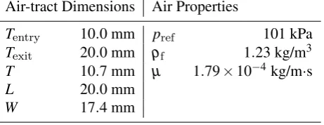
Table 1. Geometric dimensions and constitutive properties of glottal airflow model.

Air-tract Dimensions Air Properties

Tentry 10.0 mm pref 101 kPa

Texit 20.0 mm ρf 1.23 kg/m3

T 10.7 mm µ 1.79×10−4kg/m·s

L 20.0 mm

W 17.4 mm

2.1 Glottal airflow model

outlet

glottal surfaces

inlet

T

Tentry exit

x

x x

ap

ml is

(a)

(b)

ml x is x

W

Figure 1. (a) Geometry of the flow domain volume. The inlet, outlet and glottal flow-structure interaction surfaces appear as shaded. The coordinate system origin (⊗) and coordinate axes (at an offset) are shown. (b) Initial mesh of the flow domain at a coronal section

The fluid domain mass and momentum conservation equations are written in integral form, in the absence of body forces, for an arbitrary volume of fluidVf as:

I

∂(Vf₎(~v−~vg)·d

~_{S=0, (1)}

ρf

d dt

Z

Vf

~vdV+ρf I

∂(Vf₎~v(~v−~vg)·d

~_S=−I

∂(Vf₎pI·d

~_S+I

∂(Vf₎τττf·d

~_{S. (2)}

Here,~vrepresents the velocity of the fluid particle at a point with respect to a stationary ob-server andpis the static pressure measured with respect to an absolute reference pressure pref, Iis the second-order identity tensor, andτττf is the stress tensor. The density of the

fluidρf is assumed constant (incompressible) following the Boussinesq approximation.

Values used for these quantities are given in table 1. The mesh is Eulerian and the velocity of the underlying grid~vgis taken into account. In the finite volume approach variables are

typically stored at discrete cell centers. A first order upwinding interpolation scheme is used to determine face values for momentum quantities. A least-square cell-based scheme is used to compute gradients at cell centers from face values. The flow pressure at faces is determined using the pressure staggering option (or PRESTO! scheme).

To solve incompressible flow, a modified form of the SIMPLE algorithm is followed. A guess pressure field is employed, then the momentum equation (2) is advanced using this guess pressure. The resulting velocity field is not divergence-free, a requirement that follows from the continuity equation (1). To make this field divergence-free the required pressure and velocity corrections are prescribed following a predetermined strategy. In-stead of the original SIMPLE presciption, the PISO algorithm is employed to relate pres-sure and velocity corrections, with one additional iteration each for neighbor and skew-ness correction. The first order implicit scheme is used to discretize all time-derivatives and integrate over a time-increment.

initial mesh is shown in figure 1b. During the computation, mesh refinement in the near-glottis region is maintained by using layering and remeshing techniques. Typical edge length in this region is approximately 0.05 mm. The commercially available computa-tional fluid dynamics (CFD) software Ansys/FLUENT is employed to solve the glottal airflow dynamics.

2.2 Vocal fold structural model

The 3D structural domain comprises a pair of VFs with identical geometry and mesh. The geometry of one of the VFs (left) is shown in figure 2a. Specific dimensions of the VF volume appear in table 2. The geometry follows the M5 canonical model (Scherer et al 2001), with the 2D VF shape pertaining to the M5 definition extruded uniformly through the lengthL of the VF in the anterior-posterior direction. Reference points~A,~B and~C (figure 2) are identified on the medial surface of the left VF to serve as probe locations for contact pressures during VF collision. Point~Alies at(−0.740,−0.294,0.00)mm. Points

~_BandC~_{are located at a distance of 1.20 mm on either side of}~_{Aalong the anterior-posterior}

direction. A point~A′is identified on the right VF at(−0.740,0.294,0.00)mm.

A C_L

L D

T

x x x

is ap ml

C B

(a) (b)

Figure 2. (a) Three-dimensional geometry of the left half of the vocal fold (VF) model. The part of the glottal surface that is expected to contact is highlighted asCL. Locations of reference points~A,~BandC~are shown. (b) Hexahedral mesh of the

VF model. Note the higher refinement near contact-prone mid-membranous location

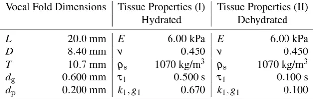
Table 2. Geometric dimensions and constitutive properties of vocal fold models.

Vocal Fold Dimensions Tissue Properties (I) Tissue Properties (II)

Hydrated Dehydrated

L 20.0 mm E 6.00 kPa E 6.00 kPa

D 8.40 mm ν 0.450 ν 0.450

T 10.7 mm ρs 1070 kg/m3 ρs 1070 kg/m3

dg 0.600 mm τ1 0.500 s τ1 0.100 s

dp 0.200 mm k1,g1 0.670 k1,g1 0.100

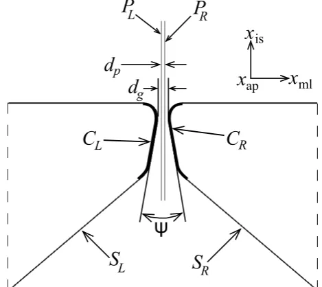
The pair of VFs are assembled as shown in figure 3. The glottal angle is ψ=−20.0◦ (converging) and the initial separation of the VFs is dg =0.600 mm. Note that W =

2D+dg, and the VF surfaces SL andSRsit flush with the flow domain boundary. Parts

of the VF exterior surfaces (CLandCR) are identified as possible contact surfaces, where

the subscriptsLandRcorrespond to left and right VF respectively.

The structural domain equilibrium equation, in the absence of body forces, is written in the weak form of virtual-work principle as

Z

Vsσσσ :δDvdV= I

∂(Vs₎~τs·δ~uvd

~_S−Z

Vsρs ¨

d

d

L

P

P

ψ

S

R

S

x

x

ml ap

x

L

C

C

Figure 3. Mid-coronal cross-section showing initial configuration: rigid planesPLandPRseparated by distancedp, the

left and right VFs separated initially by at least the gapdg and located symmetrically on either side of the respective

rigid planes, contact surfacesCLandCRon respective VFs, initial included glottal angleψand flow-structure interaction

surfacesSLandSRdefined on the respective VFs. Coordinate axes are shown offset from the origin for clarity

All variables are expressed above in the current, or deformed, configuration. Hereσσσis the Cauchy stress tensor,~τsis a externally imposed surface traction, ¨~uis the local acceleration

vector,δ~uv is a virtual displacement and δDv is the corresponding virtual deformation

gradient. Symbolsρs,Vsand∂(Vs)correspond to the density of the tissue, the deformed

configuration volume and its bounding surface respectively. In the finite element approach the equation above is first discretized in space using consistent interpolation functions that relate the value of a variable at a point with values at discrete nodes.

The acceleration vector ¨~uin (3) is used to determine the displacement~u using a time integration scheme. The time integration operator follows the implicit Hilber-Hughes-Taylorα-method (Hilber et al 1977), which allows for numerical damping. The small amount of numerical damping can effectively remove high-frequency noise from the so-lution. Damping is controlled by the parameterα=−0.41421 of the algorithm.

The commercially available finite element (FE) package ABAQUS is employed to solve the VF dynamics. Both VF volumes are meshed identically. A hexahedral element mesh (using first-order C3D8RH elements from the ABAQUS/Standard library) is used to dis-cretize the VF volumes. Increased refinement near the contact-prone mid-membranous region is present, as shown in figure 2b.

2.3 Contact interaction model

In an ideal contact model, surfacesCLandCRwould interact. Due to restrictions arising

out of numerical algorithm implementation in FLUENT, it is required that the topology of the fluid volume remains unchanged throughout the computation. Therefore, direct con-tact between surfacesCLandCRcannot be considered. Instead, as an approximation of the

true contact, a pair of auxiliary rigid planar (2D) surfaces,PLandPR, are defined to

inter-act withCLandCRrespectively. The rigid surfacesPLandPRare fixed in space and

sepa-rated bydp=0.200 m. Each rigid plane is meshed identically using rigid R3D4 elements

2.4 Boundary and coupling conditions

At any point of time during the computation, the bounding surface of the VFs∂(Vs_)can

be expressed as a union of mutually disjoint surface sets

∂(Vs) = [∂(Vs)]B∪[∂(Vs)]C∪[∂(Vs)]FSI. (4) Here,[∂(Vs_)]

B comprises the lateral (xml =±W/2), anterior (xap=L/2) and posterior

(xap=−L/2) surfaces of the VF. Throughout the computation, all degrees of freedom are

constrained for nodes on[∂(Vs_)] B. Any point~x∈∂(Vs_)−[∂(Vs_)]

Bmust satisfy the contact condition

|xml| ≥dp/2, ∀t≥0. (5)

Possibly topologically disjoint regions within∂(Vs_)−[∂(Vs_)]

B(note:∂(Vs)−[∂(Vs)]B= S

(SL,SR)), for which the equality |xml|=dp/2 is satisfied at a given instant, comprise

the surface set[∂(Vs)]Creferred to in (4). Thus[∂(Vs)]Cdenotes the surface region(s) in active contact, and is always a subset ofS

(CL,CR). The remainder of the VF bounding

surfaces is denoted by[∂(Vs_)] FSI.

The displacement condition|xml|=dp/2 on[∂(Vs)]C implies that normal surface trac-tions on[∂(Vs_)]

C are unspecified with the limitation that tensile forces are not allowed. The tangential contact interaction is frictionless, i.e. shear forces are always zero on [∂(Vs_)]

Cwhile there is no constraint on the in-plane displacement.

On[∂(Vs)]FSIthe following surface traction boundary condition is applied

~τs(t) = [−p(t+∆t)I+τττf(t+∆t)]·nˆ, (6)

where ˆnis the surface normal at a given location on the interface. The terms on the right hand side are obtained from corresponding nodes on the flow domain boundary. The dy-namic compatibility condition (6) ensures momentum balance at the FSI interface.

With the above conditions imposed on the VF boundary at time step t, equation (3) can be integrated in time to obtain the displacement and stress fields throughout the VF domain at time stept+∆t. However, equation (6) requires determination of flow variables att+∆t. The method of determination is given below.

At any timetthe flow domain boundary∂(Vf_{)can be composed as a union of mutually}

disjoint surface sets

∂(Vf) = [∂(Vf)]B∪[∂(Vf)]C′∪[∂(Vf)]FSI. (7) Here,[∂(Vf_)]

Bcomprises the flow inlet (xis=−T−Tentry), flow outlet (xis=Texit), and

non-moving walls of the entry and exit channels (xml=±W/2 andxap=±L/2)

(fig-ure 1a). The press(fig-ure at the inletpinis varied with timetas

pin(t)

pmax

=

(t/Tramp)2[3−2(t/Tramp)]∀t∈[0,Tramp]

1 ∀t∈[Tramp,∞),

(8)

wherepmax=400 Pa andTramp=0.15 s. The pressure at the outlet is constant at 0 Pa. At

all times, no slip and no penetration are prescribed on the non-moving walls of the entry and exit channels, i.e.~v=~vg=0 onxml=±W/2 and onxap=±L/2.

The kinematic compatibility condition, needed to ensure that the moving–deforming re-gions of flow boundary (∂(Vf)−[∂(Vf)]B) remain coincident with the moving–deforming regions of the VF boundary (∂(Vs_)−[∂(Vs_)]

operator in time,

~vg(t)|_∂(Vf_)−[∂(Vf_)]B=

[~u(t)−~u(t−∆t)]_∂(Vs_)−[∂(Vs_)]

B

∆t . (9)

Simultaneously, no slip and no penetration condition(~v=~vg) is imposed on (∂(Vf)−

[∂(Vf_)]

B). Further, we define[∂(Vf)]FSIas that part of the flow-domain boundary which remains coincident with [∂(Vs_)]

FSI, and [∂(Vf)]C′ is defined by its coincidence with

[∂(Vs_)]

C. It is important to note that material surface regions are exchanged between

[∂(Vs)]C and[∂(Vs)]FSI over time (for e.g.[∂(Vs)]C=/0 in the fully open state) and this results in corresponding exchange of surface sets between[∂(Vf_)]

C′and[∂(Vf)]_FSI.

With the above boundary conditions on the flow domain (requiring solid domain solu-tion~u only at instantst andt−∆t), equations (1) and (2) are integrated to obtain flow velocity and pressure at time stept+∆t. The surface traction(−pI+τττf)·nˆ att+∆t is

then computed and substituted back into (6). This updates the solid domain solution to t+∆t. Using the solid domain solution at instantstandt+∆tin (9) to obtain~vg(t+∆t)

on∂(Vf)−[∂(Vf)]Bthe flow solution can be obtained at stept+2∆t. The time integration of the coupled domain proceeds accordingly.

Equations (6) and (9) define the weak-coupling approximation employed in the present model. The surface traction(−pI+τττf)·nˆatt+∆tis used to compute the surface traction ~τsatt. As a result of staggered approach, the displacement of the solid domain boundary

is ahead of the fluid domain boundary by a single increment. The error introduced due to the mismatch in displacements is considered to be small compared to the magnitude of the total displacement integrated over time. The coupling software MpCCI is used to effect the transfer of solution variables between ABAQUS and FLUENT. The time-increment used to integrate the balance equations in both FLUENT and ABAQUS is identical to the solution exchange increment used by MpCCI. In the present computation a constant increment∆t=0.020 ms was used.

2.5 Constitutive relationships

The constitutive relation for the fluid (air) follows a Newtonian incompressible fluid pre-scription,

τττf=µ

h

∇~v+ (∇~v)Ti, (10) where µ is the dynamic viscosity. Properties of air corresponding to STP are used (ta-ble 1).

For the VF tissue a viscoelastic constitutive relation is used to define the stress-strain response,

σσσ(t) =

Z t

0

2G(t−t′)eee˙dt′+I Z t

0

K(t−t′)ε˙dt′, (11)

whereeeeis the deviatoric part of the strain, andε is the volumetric part. The second-order identity tensor is denoted byI. FunctionsG andK correspond to time-dependent shear and bulk moduli defined by a single-term Prony series

G(t) = E

2(1+ν)[1−g1+g1exp(−t/τ1)],

K(t) = E

whereEis the instantaneous small-strain elastic modulus of the VF tissue. The properties E, g1, k1 andτ1 are given numerical values such that the single-phase viscoelastic VF tissue behaves similar to a biphasic material as considered by Zhang et al (2008). The Poisson’s ratio of the VF tissueνis given a value close to the incompressibility limit of 0.50, and its densityρsis set close to that of water at STP (table 2).

In Zhang et al (2008) the stress within VF tissue – defined as a one-dimensional (1D) linear biphasic material of initial lengthL– due to an applied displacement at one end

u(L,t) =ε0

t/T0, 0≤t≤T0=0.01s

1, t≥T0, (13)

while the other end is fixed(u(0,t) =0)is given by

σ(t≥T0) = HAε0

L +

HAε0 L

2e−π2kHAt/L2+π2kHB

L2 T0π2_kH

A

×

1−φ f

φs

π2_kH

B

L2_+π2_kH

B

eT0π2kHA/L2+π2kHB₋₁

, (14)

where only the first term is retained for the sake of simplicity. Here,HA=λs+2µsand

HB = (λf+2µf)(φs/φf)

2

are respectively the moduli of the solid and fluid phases in terms of the usual elastic constants (solid) and viscosity coefficients (fluid),φs _{and φ}f are the volume fractions of the solid and fluid phases respectively andkis the hydraulic permeability of the solid phase. For water,λf=−2µf/3 (Schlichting 1989).

For the displacement condition (13), the stress on a VF tissue defined as an equivalent single-phase viscoelastic solid is found by integrating (11) to be

σ(t≥T0) =Eε0 L

1−k1+

k1τ1 T0

(eT0/τ1_−1)e−t/τ1

. (15)

Expressions (14) and (15) are equivalent under two limits. In the first case, assuming a fluid volume fraction typical of a ‘hydrated’ VF tissueφf _{=70% (Hanson et al 2010;} Phillips et al 2009), with hydraulic permeabilitykin the range given in literature (Zhang et al 2008; Tao et al 2009), andL equal to the VF length (as in table 2), it follows that π2_kH

B≪L2. This limit is modeled by the choice of parameters corresponding to model I to table 2. In the second case, assuming a severely dehydrated VF tissueφf_{→0, it follows} thatπ2_kH

B≫L2. Model II property values in table 2 simulate VF tissue in this limit. A detailed treatment of accuracy concerns regarding various parts of the computational FSI model can be found in appendix C.

3. Results

It must be noted that the time-independent elastic modulusE and Poisson’s ratio ν of the VF tissue is identical for models I and II. Therefore both models have identicalin vacuoeigenfrequencies, the first of which is 47 Hz. However, in the FSI computations, the frequency of vibration is an outcome of the coupled model, and differences are expected between the models. Computational results are presented first for the computation with tissue parameters representing a hydrated tissue (model I). An FSI computation over a physical duration of 286 ms is presented.1 During the ramp phase, the VFs deform from

1_{The computation ran for about 50 hours of CPU time, with 9 cores (4 for FLUENT, 4 for ABAQUS and 1 for MpCCI)}

their rest state, thereby bulging upward (figure 4a). The overall mean deformation of the VFs are nearly symmetric to each other. Vibrations (int≥Tramp) occur around this mean

state.

(a)

(b)

v [m/s]

|u| [m]

ψ

’

Figure 4. Att=Tramp: (a) contours of displacement magnitude corresponding to the mean deformed shape, (b) contours

of inferior-superior component of glottal airflow velocity on the mid-coronal section.

Figure 4b depicts a typical flow field in the mid coronal section of the model I before vi-bration onset. Considering the mid-coronal section in the mean deformed state (figure 4a), the included angle between the VFs isψ=20.8◦, only slightly increased when compared to the rest state (ψ =20.0◦). Flow measurements over a large range of included glottal angles with rigid models having M5 geometries were reported in Fulcher et al (2010). These authors suggests that for a converging case ofψ =20.0◦, the flow pressure near location~A(the glottal exit) is less than that at the flow domain outlet. The pressure dif-ference between glottal exit and outlet is about 10% of the pressure difdif-ference between the inlet and outlet. Therefore, the maximum pressure drop occurs between the inlet and glottal exit and is approximately 1.1pmax. Bernoulli’s theorem is expected to be valid up

Thereby, the approximate relation holds,

1.1pmax≈

1 2ρf(q

2

2−q21), (16)

whereq1andq2are average flow speeds through the inlet and glottal exit sections respec-tively. Mass continuity dictates that the mass flow rate at every cross-section perpendicular to the streamwise direction must be identical,

˙

m=ρfA1q1=ρfA2q2, (17)

whereA1 and A2 are the respective cross-section areas at the inlet and glottal exit. The mean opening between the VFs at mid-coronal plane ¯d≃2|xml(~A)|=0.732 mm. Thereby

A2 can be approximated asLd¯, assuming a rectangular opening. Using (16) and (17), it can be shown that

˙

m2=2ρf(1.10pmax)A 2 1A22 A2

1−A22

(18)

relating the mean mass flow rate with the inlet pressure. The estimated mean mass flow rate from this simple model is 0.480 g/s.

0.19 0.2 0.21 0.22 0.23 0.24 0.25 0.26 0.27 0.28

2 3 4 5 6 7 8 9 x 10

−4

computed predicted

time [s]

mass flow rate [kg/s]

Figure 5. Comparison of computed mass flow rate in dependence of time (solid line) and its predicted mean value using Bernoulli’s theorem (16) (dashed line)

The computed mass flow-rate at the inlet in dependence of time is shown in figure 5. The computed mass flow rate averaged over the cycles shown is ˙mcomputed=0.575 g/s.

The corresponding computed average volume flow rate of 471 ml/s. The average mass flow rate based Reynolds number is Re=m˙computed/Lµ ∼1600. The peak centerline

velocity component in thexisdirection was found to be∼31 m/s.

The post-ramp motion of the VFs develops in time to be soon dominated by a single fre-quency oscillation. This is also evident from the fluctuations in flow rate shown in figure 5. The time variation of distance between point~Aon the left VF and the planePLis plotted

0.190 0.2 0.21 0.22 0.23 0.24 0.25 0.26 0.27 0.28 1

2 3 4 5 6x 10

−4

time [s]

contact opening distance [m]

left right

Figure 6. Contact opening distance in dependence of time: solid line, at reference point~Aon left vocal fold; dashed line, at point~A′on right vocal fold

constant throughout the computation (SD 1.16%). At three instants of a collision-free vi-bration cycle, in particular, att=0.19626 s, 0.19772 s and 0.19920 s, the mid-coronal sections of the left VF are shown in figure 7. These instances correspond to, respectively, the maximum open state, the mean state, and the least open (or closed) state. Approxi-mating the motion of the right VF to be symmetric, the corresponding included glottal angles(ψ)at these instants are 13.1◦, 20.1◦ and 26.9◦, respectively. Though the glottal angles remain convergent, there is significant change in the degree of convergence over the vibration cycle. The amplitude increases with time such that after some cycles it is large enough to result in collision. As seen in figure 6, collision becomes well-established in the cycle beginning att=0.27986 s.

(a)

(b)

(c)

Figure 7. Glottal angle changes significantly during each phonatory cycle. Deformed shapes of the mid-coronal section at three different instants corresponding to: (a) maximum open state att=0.19626 s, (b) mean state att=0.19772 s and (c) maximum closed state att=0.19920 s.

0.2450 0.250 0.255 0.260 0.265 0.270 0.275 0.280 0.285

0.5 1 1.5

2

time [s]

area [mm

2 ]

0.242 0.244 0.246 0.248 0.25 0.252 0.254 0.256 0.258 0.26 0.262 0

600 1200 1800

time [s] (a)

pressure [Pa]

0.264 0.266 0.268 0.27 0.272 0.274 0.276 0.278 0.28 0.282 0.284 0

600 1200 1800

time [s] (b)

pressure [Pa]

A

B

C

A

B

C

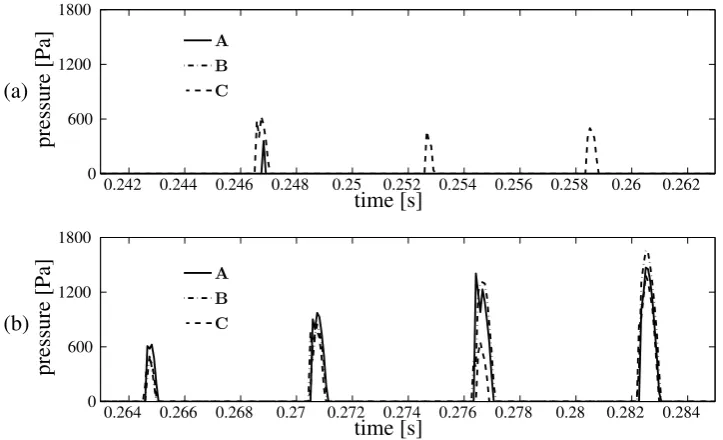
Figure 9. Time history of contact pressures measured at locations~A,~BandC~of the left VF through (a) three consecutive collision cycles, and (b) four subsequent cycles

Figure 10. Att=0.19772 s, distribution of hydrostatic stress on several transverse planes (1 mm intervals)

Figure 8 shows the time variation of the area of the left VF under contact for seven con-secutive collision cycles. The three-dimensionality of the airflow noted earlier includes an anterior-posterior asymmetry in VF deformation, and thereby VF collision. The asymme-try also causes different contact pressures at~Band~C. Contact area being a global measure does not capture this asymmetry, but is seen clearly in the contact pressure history fig-ure 9. The asymmetry develops over subsequent cycles, in that the location of contact pressure peak within a cycle changes between~A,~Band~C. The within-cycle peak contact pressure computed at~Ais found to be between 0.3 kPa and 1.5 kPa. The duration within which the left VF contacts with the planePL at~A(in each cycle) – when expressed as a

percentage of the cycle time – is at most 13.4%. This corresponds to an open quotient of at least 86.6%.

Hydrostatic stress is defined

σH= 1

where σi j is the Cauchy stress tensor σσσ written in the Einstein notation. The repeated index in (19) denotes a summation. Biot’s poroelastic theory (1941) specifies that the solid and fluid constituents of the poroelastic VF tissue exert an equal, opposite and non-zero force on each other. The theory employs Darcy’s law to relate this non-non-zero force, given by the gradient of hydrostatic stress, to the interstitial fluid flux

~q∝ ∇∇∇σH, (20)

where~qis the flux vector of the interstitial fluid. Instantaneous interstitial fluid flux fields are determined, and transport of pore fluid over time due to its motion is neglected. Thereby, local hydraulic permeability and fluid volume fraction are assumed constant, and can be absorbed into any multiplicative constant associated with (20).

With respect to figure 6, consider one typical vibration cycle free of collision (from t=0.19626 tot=0.20212) and one vibration cycle with fully developed collision (from t=0.27986 s tot=0.28578 s). The distribution of hydrostatic stress att=0.19772 s, i.e. the mean vibration state, is shown in figure 10. The contours ofσH are given at sev-eral inferior-superior cross-sections of the left VF. It is found that the levels ofσH are rather independent of the anterior-posterior location in the VF, and thus anterior-posterior gradients are small. This is in contrast to the distribution of the hydrostatic stress on the medial-lateral plane.

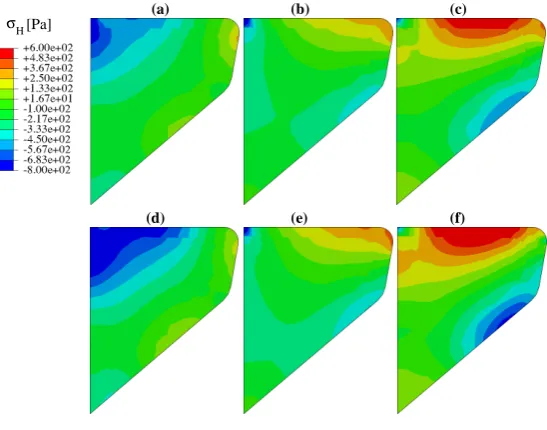
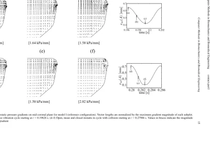
Figure 11a–c show the distribution of hydrostatic stresses on the mid-coronal plane at the maximum open, mean, and closed states of the free-vibration cycle (t=0.19626 s, 0.19772 s and 0.19920 s). Figure 11d–f shows hydrostatic stress contours on the mid-coronal plane at corresponding states of the cycle with VF collision: maximum open at t=0.27986 s, mean state at 0.28134 s, and closed at 0.28264 s. The hydrostatic stresses change significantly over the mid-coronal plane. Local hydrostatic stress gradients∇∇∇σH, proportional to interstitial flux vectors~q, are visualized over a selected region of the mid-coronal plane (figure 12) close to the VF medial surface. The anterior-posterior component of∇∇∇σH and~qare neglected in the following as their magnitude is significantly less than that of the in-plane gradient. For each instant considered, the maximum of the vector mag-nitudes is used to normalize the hydrostatic stress gradient vectors at the given instant. The vectors also represent normalized instantaneous interstitial fluid flux vectors at the

corre-(a)

(d) (e) (f)

(c) (b)

[Pa] σ_H

2012

15:21

Computer

Methods

in

Biomechanics

and

Biomedical

Engineering

contact-part1

Computer

Methods

in

Biomec

hanics

and

Biomedical

Engineering

15

(a)

(b)

[1.64 kPa/mm] [σH = 1.12 kPa/mm]

(c)

[1.58 kPa/mm]

(d)

[1.24 kPa/mm]

(e)

[1.50 kPa/mm]

(f)

[2.02 kPa/mm]

0.196 0.198 0.2 0.202

0.1 0.3 0.5 0.7

time [s]

xm

l

(

A

)

[m

m

]

(a)

(b) (c)

0.28 0.282 0.284 0.286 0.1

0.3 0.5 0.7

time [s]

xm

l

(

A

)

[m

m

]

(f) (e) (d)

sponding time instants. In figures 12a–c, the largest gradient vector is always directed to-wards the medial surface, and its magnitude changes by about 46 % between its maximum and minimum values during the cycle. It is thereby inferred that the predominant gradient is caused by the mean deformation of the VF. Indeed, this large gradient is substantial in the mean states of both the vibration and collision cycle (figures 12b,d). Comparing the open and closed states of the cycle without contact (figures 12a,c), a secondary interstitial fluid flux is apparent. This flux is aligned approximately along the inferior-superior axis and switches sense every half-cycle. In the open state, the superior surface is in relative compression, and this directs the interstitial fluid inferiorly. The situation is reversed in the closed state, and flux vectors point superiorly. This secondary fluid flux is understood to be associated with vibration. Comparing figures 12a,d the arrows directed away from the superior surface are found to be larger in the collision cycle case. This is expected since the amplitude of vibration is larger in the collision cycle, causing the magnitude of the secondary flux (relative to the rather constant mean flux) to be larger during the collision cycle. Figure 12f shows a strong tertiary interstitial fluid flux. This flux is associated with VF surface collision, which modifies the hydrostatic stress state locally. This interstitial fluid flux component is large in magnitude (about 63 % larger than the maximum flux in the open state) directed opposite to the primary fluid flux direction, i.e. away from the medial surface during collision. The influence is limited spatially to within a zone sur-rounding the location of collision (see figure 12c,f), and temporally to within the duration the particular location is in contact. Outside this spatio-temporal zone interstitial fluid flux characteristics resemble those of a free-vibration cycle.

Results from the FSI simulation considering properties of a dehydrated tissue (model II) are presented below. Only some select variables are detailed herein that emphasize the contrast with respect to the hydrated tissue (model I). The mean opening between the VFs at the mid-coronal plane and the mean mass-flow rate are ¯d=0.852 mm and

˙

mcomputed =0.676 g/s respectively. The frequency of vibration for model II is 108 Hz,

the peak contact pressures are in the range 0.5–2.0 kPa and open quotients are at least 75.5 %.

The hydrostatic stress gradient derived interstitial fluid flux vectors are considered at in-stants 0.25480 s, 0.25710 s and 0.25940 s that represent fully open, mean and maximum closed states respectively within a collision-free vibration cycle of model II. For respec-tive states within a cycle with collision, instants 0.28170 s, 0.28400 s and 0.28570 s are considered. The normalized interstitial fluid flux vectors are shown in figure 13(a)–(c) and (d)–(f) respectively for the collision-free cycle and the cycle with collision. The cycles are selected such that the amplitudes of vibration about the mean are comparable to those in corresponding cycles in figure 12 (model I).

Comparison of figures 12 and 13 indicate that the overall fluid flux directions were not altered by changing the tissue properties. However, significant changes in the spatial distribution of flux magnitudes are found. For the free vibration conditions, the magnitude of flux is significantly reduced for all instances considered (−19 %,−42 %,−37 % for the open, mean and closed states, respectively), with the strongest reduction occurring at the mean state. Furthermore, the flux magnitudes are less equally distributed spatially in the dehydrated state with the highest flux rates highly concentrated closely to the medial plane.

2012

15:21

Computer

Methods

in

Biomechanics

and

Biomedical

Engineering

contact-part1

Computer

Methods

in

Biomec

hanics

and

Biomedical

Engineering

17

H

(a) (b) (c)

(d) (e) (f)

[σ = 0.901 kPa/mm] [0.941 kPa/mm] [0.985 kPa/mm]

[0.672 kPa/mm] [0.873 kPa/mm] [2.60 kPa/mm]

0.254 0.258 0.262

0.1 0.3 0.5 0.7

time [s]

xm

l

(

A

)

[m

m

]

(a)

(b) (c)

0.282 0.286 0.29

0.1 0.3 0.5 0.7 0.9 1.1

time [s]

xm

l

(

A

)

[m

m

]

(e) (f) (d)

4. Discussion

The present study documents FSI computations of VF vibrations under realistic condi-tions. For computations considering a hydrated tissue (model I), the average mass flow rate based Reynolds number was found to compare well with Re∼O(103) measured in physical experiments (Alipour and Scherer 1995; Cranen and Boves 1985; Triep and Br¨ucker 2010). The computed peak centerline velocity component in thexis direction is

typical of measured values in experiments (Erath and Plesniak 2006; Pelorson et al 1994). The computed average volume flow rate is well within the 80−750 ml/s range measured in experiments using excised larynges and physical replicas of VFs (Alipour and Scherer 1995; van den Berg et al 1957; Cranen and Boves 1985; Erath and Plesniak 2006, 2010; Triep et al 2005) and computed using numerical models (Scherer et al 2001; Thomson et al 2005; Triep and Br¨ucker 2010). The three-dimensional development of the com-puted glottal jet was also observed in experiments (Krebs et al 2012; Triep and Br¨ucker 2010). The frequency of vibration as computed falls within the range of realistic phonation frequency (George et al 2008; Morris and Brown Jr. 1996; Titze 2006; Zhang et al 2006). The vibration amplitude is in the range of measured values (Alipour et al 2001; Baer 1981; George et al 2008). The computed peak contact pressures were in the range of mea-sured (Gunter et al 2005; Jiang and Titze 1994; Spencer et al 2006; Verdolini et al 1999) and computed values (Chen 2009; Gunter 2003; Hor´aˇcek et al 2005). The computed open quotients were at the higher end of the 28−93% range observed in experiments (Hanson et al 1990; Henrich et al 2005; Verdolini et al 1998). For the dehydrated tissue condition (model II) the above variables were also found to be within the range of values measured in experiments. However, it was evident that a change in the underlying tissue character-istics could result in significantly different vibration charactercharacter-istics even when the airflow conditions were kept identical. In particular, it was found that a dehydrated VF tissue vi-brated with a lower frequency than the hydrated tissue. The mean opening between the VFs during vibration was also higher for the dehydrated case, which perhaps explains the higher mean volume air flow rate through the glottis compared to the hydrated case.

The average air flow rate, which remains constant post ramp, was compared with Bernoulli’s approximation for steady flow. The flow during free-vibration and collision cycles is not steady in a strict sense. However, the so-called quasisteady approximation has been found to hold for the glottal air-flow (McGowan 1993). The quasisteady approxi-mation states that the instantaneous flow field though a vibrating glottis is not significantly altered if the deformation of the glottis is frozen in time. The physical implication of the approximation is that at any instant the constriction in the glottal channel provides a larger flow acceleration relative to the time- dependent VF motion. Mathematically, this means that the time-derivative of velocity potential in the unsteady Bernoulli equation (Batchelor 2010) is relatively small compared to the other terms. The 18.0 % difference between the computed and approximated values of average flow-rate is possibly due to the fact that the unsteady effects are not entirely negligible.

the fluid is incompressible, a segregated problem will always become unstable in a finite number of time increments (F¨orster et al 2007). The instability in the computed FSI solu-tions presented in this paper cause the fluctuation amplitude of displacement and stresses to grow with time for both cases considered. This limitation is inherent in a segregated ap-proach. In an ideal case, a finite but stable amplitude of vibration is likely to be observed. However, in the present case the instability is weak. A rough estimate of the amplitude growth rate can be obtained from figure 6. The amplitude of vibration (about the mean distance∼0.25 mm) for the first cycle is∼0.2 mm. Assuming the mean to be identical for the last cycle the fluctuation amplitude is∼0.37 mm, i.e. and increase of∼1.8 times over 15 vibration cycles. Therefore, on an average, the amplitude of vibration increases by∼3.9% between subsequent cycles. The time-constant associated with this growth rate is much smaller than the vibration period. As the VF vibration amplitude increases, the fluctuation in the flow rate is also found to increase, at a rate which is indistinguishable from the rate of increase of VF vibration amplitude. This implies that flow rate fluctua-tion remains linearly proporfluctua-tional to the VF vibrafluctua-tion amplitude. Further, throughout the computation the average flow rate and mean VF vibration amplitude remains steady. It can be argued that the present computation determines the state of stress in an experi-mental model with identical geometry, material properties and average flow rate. Such a determination is possible by selecting a particular computed cycle for which the flow-rate fluctuation amplitude matches the experimentally measured flow-rate fluctuation ampli-tude. For this specific computed cycle, the VF motion would match that of the experiment. The state of stress corresponding to this particular cycle is hence physically relevant.

The problem of unstable response is also relevant because the onset of phonation is in itself a instability event. Phonation onsets when the transglottal pressure difference goes above a certain value. This value, or phonation threshold pressure (PTP), is a function of the dynamical system (tissue properties, geometry, boundary conditions, etc.). Although in the VF FSI problem the density ratio of structure and fluid and structural stiffness are favorable in mitigating the role of numerical instability, it is difficult to reliably predict physical instability (onset) in the presence of numerical instability. Therefore the phona-tion onset problem is not addressed in this paper. This is not a shortcoming because the phonation onset problem is independent of the problem of determining stresses that de-velop in a readily self-oscillating VF post the onset. For transglottal pressure difference above PTP, the frequency and amplitude of vibration in self-oscillation are not externally imposed conditions; rather they appear as part of the solution. This is highlighted in the present computations where the two models considered have significant differences in fre-quencies of vibration and average deformation, although theirin vacuoeigenfrequencies based on the instantaneous elastic properties are identical.

The FSI computation framework employed in this paper allows for detailed determi-nation of the spatial and temporal evolution of stresses in the interior of the VFs. In par-ticular, hydrostatic stresses and their gradients are considered. The poroelastic nature of VF tissue motivates the use of hydrostatic stress gradients to determine the flux at which interstitial fluid flows relative to the solid matrix. Distribution of hydrostatic stress at three representative instants (corresponding to open, mean and closed states) of free-vibration cycles and collision cycles were presented for the two VF tissue characteristic states (hy-drated and dehy(hy-drated). These results underline the following implications on the intersti-tial fluid flux within the VF tissue:

(1) Interstitial fluid flux along a coronal plane is typically stronger that out of it. This is because the hydrostatic stress gradients in the anterior-posterior direction were found in general to be weaker compared to those in the mid-coronal plane. (2) Within the mid-coronal plane, the sense of the gradient in the mean state dictates

gradients of hydrostatic stress in the anterior-posterior direction are small. (3) A secondary interstitial fluid flux is aligned approximately along the

inferior-superior axis and switches sense every half-cycle. The strength of this flux scales with the magnitude of vibration around the mean state. It aids in the uniform distribution of interstitial fluid throughout the VF volume.

(4) A tertiary interstitial fluid flux results from collision at the VF surface. The collision-induced flux operates only within a zone surrounding the location of col-lision (see figures 12c,f and 13c,f), and while the particular location is in contact. This flux component is directed against the mean deformation induced primary flux.

The degree of severity of collision can be quantified through the extent of the spatio-temporal zone of influence of reversed interstitial fluid flux, and also the magnitude of change in stress caused by collision. The extent of the spatio-temporal domain of influ-ence of collision is in turn determined by the specific phonation conditions. For example, by changing the initial pre-phonatory distance between the VFs, the fraction of cycle-time for which contact occurs and the spatial depth of influence is modified, while keeping vibration amplitude and mean deformation constant. Open quotients smaller than those computed in this paper, and well-within the experimentally observed range, can be ex-pected to result in more severe collision. The effect of moderate collision (as considered here) on the interstitial fluid flux is strong relative to the mean flux. Collision can thereby be expected to play an effective role in removing fluid from the medial surface.

The differences between figures 12 and 13 highlight the effect of tissue viscoelastic properties, and thereby its hydration state. Specifically comparing the maximum open state in the collision-free cycles in figures 12a and 13a, respectively, it is observed that the increase in stress gradient magnitude near the medial surface as compared to the rest of the mid-coronal section is even higher in the dehydrated than in the hydrated state. This is true in general for other states when the mid-coronal section is not in active contact. In the dehydrated state collision-induced stresses are seen to play a stronger role in dehydrating the VF tissue compared to the hydrated state. A plausible biomechanical implication is that severe dehydration of VF tissue can lead to even higher levels of dehydration leading to potential tissue damage. Such implications could be investigated in future through care-fully designed experiments. Although it is not reasonable to draw definitive conclusions regarding VF biomechanics based solely on present computations, it must be emphasized that specific quantitative comparisons such as the above can only be made by conduct-ing FSI computations presented herein, and cannot be determined from simplified models considering gross pressure differences in the system.

The interstitial fluid flux in Darcy’s equation (20) is, strictly speaking, proportional to the gradient of that part of the total hydrostatic stress(σH)which is supported by the fluid constituent. The fluid-supported hydrostatic stress, as fraction of the total stress, changes with time. Therefore, it can be argued that the proportionality in (20) includes a time-dependent factor. Indeed, in Zhang et al (2008) it was shown that this time-dependence is given by an exponential decay (see figure 7 in Zhang et al 2008). The time-constant for the exponential decay is given byτ1, whereas the time period of vibration is 1/f. For models I and II the ratio of the time-scales 1/(fτ1) is 1.20 % and 9.26 % respectively. This ratio is representative of the percentage decay in fluid-supported stress, as a fraction of the total stress, within a single cycle of vibration. Therefore, the stress on the fluid constituent effectively remains a constant fraction ofσH. This implies that comparison of interstitial fluid flux derived from (20) is a close measure of the fully coupled problem.

finite but small distancedp. The effect of this difference compared to the real situation

(dp =0), on the development of local collision effects and the development of overall

FSI is discussed in appendices A and B respectively. In Shurtz and Thomson (2012) it was demonstrated, using a two-dimensional computational model, that the VF dynamics had negligible sensitivity to the choice ofdp in the range considered. Both models I and

II can be compared with that in Shurtz and Thomson (2012) by considering the quantity dp/dg. In the present casedp/dg=0.33 was within the range ofdp/dg(from 0.01 to 0.50)

considered by Shurtz and Thomson (2012). Thereby Shurtz and Thomson (2012) support the arguments made in appendices A and B.

Another important aspect of the current framework, and in particular with respect to the VF tissue constitutive relations, is that realistic viscoelastic properties were used and that a full 3D geometric description was included. Deformation asymmetry in the anterior-posterior direction, absent in 2D models reported in literature, emphasizes the importance of three-dimensionality. In agreement with Erath et al (2011b,a), the asymmetry in the air flow and the jet attachment in the medial–lateral direction (Coanda effect) did not result in significant asymmetry of deformation between the left and right VFs. In the airflow model, the dynamic viscosity of air was considered at its realistic value. Consequently, the Reynolds number of the flow turned out to be representative of experimental FSI con-ditions. The Reynolds number determines length and time scales of dynamic events in a laminar flow, and Buckingham’s Pi-theorem stipulates that it is impossible to determine a single scaling factor that can be applied to both air flow and tissue properties and yet keep unchanged the relevant non-dimensional numbers of the fully coupled flow-structure in-teraction system (Erath and Plesniak 2010). In this light, modifying the Reynolds number in FSI computation of phonation removes the correspondence between dynamics of the computational model and the physical system it attempts to model.

The results present quantitative data on the dynamic state of stresses inside a pair of VFs with realistic 3D geometry and tissue properties obtained during flow-induced vibration and collision. Validation with a carefully designed experimental replica is the best way to resolve any questions regarding the physical relevance of the results presented herein. In the paper it was shown that, wherever such a comparison is possible, the results from the computation do agree with measurements made on similar experimental models.

5. Conclusion

hand, previous studies (Solomon and DiMattia 2000) have found that the effect on voice competence measures (for example, PTP) due to tasks demanding higher voice intensity can be offset by increased hydration of the VFs. Hanson et al (1990) found that increased voice intensity is associated with lower open quotients, whereas Verdolini et al (1998) found that decrease in open quotient was related to increase in contact stresses measured on the VF surface. These observations taken together indicate that, from the perspective of vocal health, increase in severity of collision is detrimental, whereas the avoidance of excessive collision is beneficial. A biomechanical explanation for these clinical findings is given in the present paper.

Acknowledgements

This work was funded by NIDCD Grant 5R01DC008290-05.

References

Alipour F, Scherer RC (1995) Pulsatile airflow during phonation: an excised larynx model. J Acoust Soc Am 97(2):1241– 1248

Alipour F, Montequin D, Tayama N (2001) Aerodynamic profiles of a hemilarynx with vocal tract. Ann Otol Rhinol Laryngol 110(6):550–555

Argentina M, Mahadevan L (2005) Fluid-flow-induced flutter of a flag. P Natl Acad Sci USA 102(6):1829–1834 Baer T (1981) Observation of vocal fold vibration: measurement of excised larynges. In: Stevens KN, Hirano M (eds) Vocal

fold physiology, University of Tokyo Press, chap 10, pp 119–132

Bartlett RS, Thibeault SL (2011) Bioengineering the vocal fold: A review of mesenchymal stem cell applications. In: George A (ed) Advances in biomimetics, InTech, chap 22, pp 473–488

Batchelor GK (2010) Introduction to fluid dynamics, 14th edn. Cambridge University Press, Cambridge

Bathe KJ, Zhang H, Ji S (1999) Finite element analysis of fluid flows fully coupled with structural interactions. Comput Struct 72(1–3):116

van den Berg J (1958) Myoelastic-aerodynamic theory of voice production. J Speech Hear Res 1(3):227–244

van den Berg J, Zantema JT, Doornenbal Jr P (1957) On the air resistance and the Bernoulli effect of the human larynx. J Acoust Soc Am 29:626–631

Biot MA (1941) General theory of three-dimensional consolidation. J Appl Phys 12(2):155–164

Branski RC, Verdolini K, Sandulache V, Rosen CA, Hebda PA (2006) Vocal fold wound healing: A review for clinicians. J Voice 20(3):432–442

van Brummelen EH, Geuzaine P (2010) Fundamentals of fluid-structure interaction, John Wiley & Sons, Ltd

Chan RW, Tayama N (2002) Biomechanical effects of hydration in vocal fold tissues. Otolaryng Head Neck 126(5):528–537 Chen LJ (2009) Investigations of mechanical stresses within human vocal folds during phonation. PhD thesis, Purdue

University

Chen LJ, Mongeau L (2009) Measurements of the contact pressure in human vocal folds. In: EMBC: 2009 Conf. Proc. IEEE Eng. Med. Biol. Soc., vol 1–20, pp 869–872

Cranen B, Boves L (1985) Pressure measurements during speech production using semiconductor miniature pressure trans-ducers: Impact on models for speech production. J Acoust Soc Am 77(4):1543–1551

Dejonckere PH, Kob M (2009) Pathogenesis of vocal fold nodules: new insights from a modeling approach. Folia Phoniatr 61(3):171–179

Dikkers FG, Hulstaert CE, Oosterbaan JA, Cervera-paz FJ (1993) Ultrastructural changes of the basement membrane zone in benign lesions of the vocal folds. Acta Oto-laryngol 113(1–2):98–101

Drechsel JS, Thomson SL (2008) Influence of supraglottal structures on the glottal jet exiting a two-layer synthetic, self-oscillating vocal fold model. J Acoust Soc Am 123:4434–4445

Elliot N, Sundberg J, Gramming P (1995) What happens during vocal warm-up? J Voice 9(1):37–44

Erath BD, Plesniak MW (2006) The occurrence of the Coanda effect in pulsatile flow through static models of the human vocal folds. J Acoust Soc Am 120(2):1000–1011

Erath BD, Plesniak MW (2010) An investigation of asymmetric flow features in a scaled-up driven model of the human vocal folds. Exp Fluids 49:131–146

Erath BD, Peterson SD, Zanartu M, Wodicka GR, Plesniak MW (2011a) A theoretical model of the pressure distribu-tions arising from asymmetric intraglottal flows applied to a two-mass model of the vocal folds. J Acoust Soc Am 130(1):389–403

Erath BD, Zanartu M, Peterson SD, Plesniak MW (2011b) Nonlinear vocal fold dynamics resulting from asymmetric fluid loading on a two-mass model of speech. Chaos 21(3):033,113

F¨orster C, Wall WA, Ramm E (2007) Artificial added mass instabilities in sequential staggered coupling of nonlinear structures and incompressible viscous flows. Comput Meth Appl Mech Eng 196:1278–1293

Fulcher LP, Scherer RC, Witt KJD, Thapa P, Bo Y, Kucinschi BR (2010) Pressure distributions in a static physical model of the hemilarynx: Measurements and computations. J Voice 24(1):2–20

George NA, de Mul FFM, Qiu Q, Rakhorst G, Schutte HK (2008) Depth-kymography: high-speed calibrated 3D imaging of human vocal fold vibration dynamics. Phys Med Biol 53:2667–2675

Gray SD, Titze IR (1988) Histologic investigation of hyperphonated canine vocal cords. Ann Oto Rhinol Laryn 97(4):381– 388

Gunter H (2003) A mechanical model of vocal fold collision with high spatial and temporal resolution. J Acoust Soc Am 113(2):994–1000

Gunter HE, Howe RD, Zeitels SM, Kobler JB, Hillman RE (2005) Measurement of vocal fold collision during phonation: Methods and preliminary data. J Speech Lang Hearing R 48(3):567–576

Hanson DG, Gerratt BR, Berke GS (1990) Frequency, intensity, and target matching effects on photoglottographic measures of open quotient and speed quotient. J Speech Lang Hear R 33:45–50

Hanson KP, Zhang Y, Jiang JJ (2010) Parameters quantifying dehydration in canine vocal fold lamina propria. Laryngoscope 2010:1363–1369

Henrich N, d’Alessandro C, Doval B, Castellengo M (2005) Glottal open quotient in singing: Measurements and correlation with laryngeal mechanisms, vocal intensity, and fundamental frequency. J Acoust Soc Am 117(3):1417–1430 Hilber HM, Hughes TJR, Taylor RL (1977) Improved numerical dissipation for time integration algorithms in structural

dynamics. Earthquake Eng Struc 5(3):283–292

Hor´aˇcek J, ˇSidlof P, ˇSvec JG (2005) Numerical simulation of self-oscillations of human vocal folds with Hertz model of impact forces. J Fluids Struct 20:853–869

Hor´aˇcek J, Laukkanen AM, ˇSidlof P, , Murphy P, ˇSvec JG (2009) Comparison of accelaration and impact stress as possible loading factors in phonation: a computer modeling study. Folia Phoniatr 61(3):137–145

Jiang JJ, Titze IR (1994) Measurement of vocal fold intraglottal pressure and impact stress. J Voice 8(2):132–144 Jiang JJ, Shah AG, Hess MM, Verdolini K, Banzali FM, Hanson DG (2001) Vocal fold impact stress analysis. J Voice

15(1):4–14

Krebs F, Silva F, Sciamarella D, Artana G (2012) A three-dimensional study of the glottal jet. Exp Fluids 52(5):1133–1147 Leydon C, Sivasankar M, Falciglia DL, Atkins C, Fisher KV (2009) Vocal fold surface hydration: A review. J Voice

23(6):658–665

Luo H, Mittal R, Zheng X, Bielamowicz SA, Walsh RJ, Hahn JK (2008) An immersed-boundary method for flow-structure interation in biological systems with application to phonation. J Comput Phys 227:9303–9332

Luo H, Mittal R, Bielamowicz SA (2009) Analysis of flow-structure interation in the larynx during phonation using an immersed boundary method. J Acoust Soc Am 126(2):816–824

McGowan RS (1993) The quasisteady approximation in speech production. J Acoust Soc Am 94(5):3011–3013

Miri AK, Barthelat F, Mongeau L (2012) Effects of dehydration on the viscoelastic properties of vocal folds in large deformations. J Voice 26(6):688–697

Morris RJ, Brown Jr WS (1996) Comparison of various automatic means for measuring mean fundamental frequency. J Voice 10(2):159–165

Noordzij JP, Ossoff RH (2006) Anatomy and physiology of the larynx. Otolaryng Clin N Am 39:1–10

O’Connor K (2012) Caring for your voice. http://www.singwise.com/cgi-bin/main.pl?section=articles&doc=CareForVoice, accessed January 23, 2012

Pelorson X, Hirschberg A, van Hassel RR, Wijnands APJ (1994) Theoretical and experimental study of quasisteady-flow separation within the glottis during phonation. Application to a modified two-mass model. J Acoust Soc Am 96(6):3416–3431

Phillips R, Zhang Y, Keuler M, Tao C, Jiang JJ (2009) Measurement of liquid and solid component parameters in canine vocal fold lamina propria. J Acoust Soc Am 125(4):2282–2287

Scherer RC, Shinwari D, DeWitt KJ, Zhang C, Kucinschi BR, Afjeh AA (2001) Intraglottal pressure profiles for a symmet-ric and oblique glottis with a divergence angle of 10 degrees. J Acoust Soc Am 109(4):1616–1630

Schlichting H (1989) Boundary layer theory. McGraw-Hill

Shurtz TE, Thomson SL (2012) Influence of numerical model decisions on the flow-induced vibration of a computational vocal fold model. J Comput Struct, in press

Sidlof P, Doar´e O, Cadot O, Chaigne A (2011) Measurement of flow separation in a human vocal folds model. Exp Fluids 51:123–136

Sivasankar M, Leydon C (2010) The role of hydration in vocal-fold physiology. Curr Opin Otolaryngo 18(3):171–175 Solomon N, DiMattia MS (2000) Effects of a vocally fatiguing task and systemic hydration on phonation threshold pressure.

J Voice 14(3):341–362

Spencer M, Siegmund T, Mongeau L (2006) Determination of superior-surface strains and stresses, and vocal fold contact pressure in a synthetic larynx model using digital image correlation. J Acoust Soc Am 123(2):1089–1103 Stein K, Benney R, Kalro V, Tezduyar T, Leonard J, Accorsi M (2000) Parachute fluid-structure interactions: 3-d

computa-tion. Comput Meth Appl Mech Eng 190:373–386

Tao C, Jiang JJ, Zhang Y (2006) Simulation of vocal fold impact pressures with a self-oscillating finite-element model. J Acoust Soc Am 119(6):3987–3994

Tao C, Jiang JJ, Zhang Y (2009) A fluid-saturated poroelastic model of the vocal folds with hydrated tissue. J Biomech 42(6):774–780

Tateya T, Tateya I, Sohn JH, Bless DM (2006) Histological study of acute vocal fold injury in a rat model. Ann of Oto Rhinol Laryn 115(4):285–292

Taylor CA, Hughes TJR, Zarins CK (1998) Finite element modeling of blood flow in arteries. Comput Meth Appl Mech Eng 158:158196

Thomson SL, Mongeau L, Frankel SH (2005) Aerodynamic transfer of energy to the vocal folds. J Acoust Soc Am 118(3):1689–1700

Titze I (2006) The myoelastic aerodynamic theory of phonation. NCVS, Iowa City, Iowa Titze IR (1994) Mechanical stress in phonation. J Voice 8(2):99–105

Triep M, Br¨ucker C (2010) Three-dimensional nature of the glottal jet. J Acoust Soc Am 127(3):1537–1547

Triep M, Br¨ucker C, Schr¨oder W (2005) High-speed PIV measurements of the flow downstream of a dynamic mechanical model of the human vocal folds. Exp in Fluids 39(2):232–245

Verdolini K, Chan R, Titze IR, Hess M, Bierhals W (1998) Correspondence of electroglottographic closed quotient to vocal fold impact stress in excised canine larynges. J Voice 12(4):415–423

Verdolini K, Hess MM, Titze IR, Bierhals W, Gross M (1999) Investigation of vocal fold impact stress in human subjects. J Voice 13(2):184–202

New York Eye and Ear Infirmary, accessed January 23, 2012

Walhorn E (2002) Ein simultanes berechnungsverfahren f¨ur fluid-struktur wechselwirkungen mit finiten raum-zeit-elementen. PhD thesis, Technischen Universit¨at Carolo-Wilhelmina zu Braunschweig

Zhang Q, Hisada T (2001) Analysis of fluid-structure interaction problems with structural buckling and large domain changes by ale finite element method. Comput Meth Appl Mech Eng 190:6341–6357

Zhang Q, Hisada T (2004) Studies of strong coupling and weak coupling methods in FSI analysis. Int J Numer Meth Eng 60:2013–2029

Zhang Y, Czerwonka L, Tao C, Jiang JJ (2008) A biphasic theory for the viscoelastic behaviors of vocal fold lamina propria in stress relaxation. J Acoust Soc Am 123(3):1627–1636

Zhang Z, Neubauer J, Berry DA (2006) The influence of subglottal acoustics on laboratory models of phonation. J Acoust Soc Am 120(3):1558–1569

Zheng X, Bielamowicz S, Luo H, Mittal R (2009) A computational study of the effect of false vocal folds on glottal flow and vocal fold vibration during phonation. Ann Biomed Eng 37(3):625–642

Zheng X, Xue Q, Mittal R, Bielamowicz SA (2010) A coupled sharp-interface immersed boundary-finite-element method for flow-structure interaction with application to human phonation. J Biomech Eng 132(11):111 003

Appendix A. Error in collision characteristics due to contact enforcement condition

In this section, the the error in determining VF stresses due to the particular value ofdp

used is discussed. Note that the rigid planes interact with the VFs only during the collision cycles. Thus, only for collision cycles, can the stress distribution in the VFs have an error due to non-zerodp.

For the purpose of comparison, the physical scenario is approximated by the hypo-thetical casedp=0. This case is an approximation of the physical scenario because the

motion of the motion of the left and right VFs are not strictly symmetric. Although such a case cannot be computed by the model (due to limitations mentioned earlier), it allows systematic comparison with the computed case.

In the fully-developed collision cycle, beginning at t=0.27986 s, the VFs approach each other, collide with the respective rigid planes, and move apart until they reach the maximum open state att=0.28578 s. If att=0.28578 s the rigid planes are instanta-neously repositioned atxml=0 (such thatdp=0) for the successive cycle, the collision

characteristics are modified in two ways. Firstly, a smaller area of the VF surfaces collide, and secondly, within this reduced collision-influenced region, the compression depth is itself reduced by a distance equal todp/2.

From the biomechanics standpoint, the decreases in contact area and contact depth im-ply that the volume over which collision influences interstitial movement is overestimated in the computation. In particular, the tertiary interstitial fluid flux due to collision is ex-pected to be weaker in the physical scenario (compared to the computation). However, the primary and secondary interstitial fluid flux modes (due to mean deformation and vibration, respectively) are identical to the computation.

Appendix B. Estimate of error in FSI due to contact enforcement condition

It may be recalled that the rigid planes never interact directly with the flow domain. A non-zerodp influences the flow solution inasmuch it modifies the movement of the VF

surfaces during collision cycles. Thereby, as computed, the FSI can contain an error due to the presence of the rigid planes. A global measure of the error in FSI can be obtained by considering energy quantities, and is estimated below.

For comparison, following the discussion in appendix A, the hypotheticaldp=0 case