Volume 35, Issue 4
A monopsonistic approach to disability discrimination and non-discrimination
Eirini-Christina Saloniki
Academic Unit of Health Economics, University of Leeds
Abstract
We use a simple model of monopsony to explain wage differences between the work-limited disabled and non-disabled. In this model, employers exploit the non-work-limited disabled workers and potential workers by offering them lower wages to increase profits, knowing that they face high search costs. We propose an extension of this model to account for the case where firms are not allowed, by law, to treat disabled and non-disabled differently. We show that non-discrimination improves the wage distribution for the non-work-limited disabled workers but worsens it for the non-disabled.
I would like to thank Amanda Gosling, Mathan Satchi and José Silva-Becerra for the useful comments and discussions and two anonymous referees for their helpful suggestions.
Citation: Eirini-Christina Saloniki, (2015) ''A monopsonistic approach to disability discrimination and non-discrimination'', Economics Bulletin, Volume 35, Issue 4, pages 2064-2073
Contact: Eirini-Christina Saloniki - e.c.saloniki@leeds.ac.uk.
1. Introduction
Over the years it has been consistently reported that disabled workers receive lower wages than their non-disabled counterparts even when differences in human capital and job related characteristics are controlled (Jones 2008, Jones and Latreille 2009 and Malo and Pagan 2012). Except for the explained part of the wage gap between the disabled and non-disabled, there exists an unexplained part that is often attributed to discrimination. Discrimination can arise if employers are prejudiced against disabled workers hence have a “taste for discrimination” (Becker 1971). Based on this theory a number of studies found that at least one third of the gap was due to discrimination against the disabled workers (Johnson and Lambrinos 1985 and Baldwin and Johnson 1994,2000). However, given the interrelation between disability prejudice, severity of disability and work productivity, and its importance when decomposing the gap, DeLeire (2001) divided further the disabled into work-limited and non-work-limited. Non-work-limited disabled were defined as having a health problem that does not affect their productivity. Assuming that i) non-disabled and non-work-limited disabled are equally productive, and ii) non-work-limited disabled and work-limited disabled face the same amount of discrimination, DeLeire (2001) and Jones (2009) reported that the amount of the gap attributed to discrimination against either work-limited or non-work-limited disabled was still significant (although lower in magnitude).
Alternatively, discrimination can arise if employers find it difficult to assess the productivity of their disabled employees. They may take the participation in a disability group as a sign of lower productivity thereby discriminate against this group, known in the literature as statistical discrimination (Phelps 1972).
In this paper, we think of wage discrimination as a result of exploitation of the disabled workers by the employers to increase profits (monopsonistic approach). If discrimination is prohibited by law we show that the effect on wages will not be the same. It is appropriate to think of wage discrimination against the disabled in such framework due to the limited job mobility of workers with disabilities. Disabled face low outside options as their job mobility costs are high, or because they have strong preference for part-time jobs and self-employment to accommodate their disability (Baldwin and Schumacher 2002 and Jones and Latreille 2011). Employers know about these options and if disabled and non-disabled face the same job offer arrival rates the disabled receive lower wages, as their search costs are high. If the disabled receive less job offers than the non-disabled, they still get lower wages (monopsonistic type of market). However, employers may not be allowed by law to offer different wages to disabled and non-disabled.1
If employers are allowed to discriminate there will be two separate markets: i) non-disabled and ii) non-disabled, whereas if employers are not allowed to discriminate there will be an integrated market of disabled and non-disabled. To discuss the above mechanisms we use a simple model of monopsony (Burdett and Mortensen 1998). To our knowledge, the Burdett-Mortensen model (B-M) has been mostly used to explain gender pay differences (Barth and Dale-Olsen 2009, Hirsch et al. 2010, Ransom and Oaxaca 2010 and Sulis 2011); they have identified significant levels of market power for employers, in line with exploitation of the minority group (in this case women) to increase profits.
If disabled and non-disabled do not differ in productivities i.e. non-work-limited disabled, the aim of the paper is threefold. First, we explain wage discrimination against the under-researched group of the non-work-limited disabled using the B-M model. Second, we propose
1For example, in the UK according to the Equality Act (2010) employers are not allowed to discriminate against
an extension of this model to account for when discrimination is prohibited, and finally we report results from a simple simulation exercise to support the models’ predictions.
2. Models of monopsony
As Manning (2003) puts it “the main advantage of the monopsonistic approach is that the way one thinks about labour markets is more “natural” and less forced”, with the firm not having a perfectly elastic labour supply. A monopsonistic model, such as the one our paper is based on, makes the following assumptions: firstly, markets are not without frictions (referring to job rents) so a separation of a worker and an employer will make both parties worse off – the worker has to look for another job and the employer has to look for a new worker. Secondly, if frictions exist employers get enough market power which they exercise by setting wages prior to their meeting with the workers, and finally there is no wage bargaining.
2.1 Discrimination
In the simple B-M (1998) model, firms have identical constant returns to scale production functions with average and marginal product of workers equal to p. Workers are also identical i.e. each has the same value of leisure b. Some workers are employed and others are non-employed. Employers make wage offers to the workers and potential workers; the wage offer distribution is denoted by F(w) and the job offer arrival rate is λ. The job destruction rate is δ (movement from employment to non-employment) and is exogenous. An employed worker accepts a wage offer if it is greater than his current wage and if non-employed accepts any offer that is greater than the reservation wage R. In equilibrium, there is no point in any firm offering a wage less than b and all employers earn the same profit:
2)) ( 1 ( 1
) ( )
(
w F k
w p w
(1)
where
k , represents the ratio of the arrival rate to the job destruction rate i.e. the inverse of the so called market friction parameter.
When wRb, (1) becomes:
2)) ( 1 ( 1
) ( )
(
b F k
b p b
(2)
with F(b)0.
After setting (1) equal to (2) and some further calculations, the equilibrium wage offer distribution is given by the following condition:
b p
w p k
k w
F( ) 1 1 (3)
The fraction of employed workers receiving wage w or less is G(w). G(w) differs from )
(w
F because workers are more likely to work for high wage firms. Also, there is a monotonic relationship between F and G as shown below:
)] ( 1 [ 1
) ( )
(
w F k
w F w
G
with G(w)F(w) for any 0F(w)1.
After substituting (3) to (4) we get the equilibrium wage distribution:
1 1
) (
w p
b p k w
G (5)
Using (4) and F(w)1, with w being the largest wage paid, we can also show that in equilibrium the offer wages should lie in the interval:
( )
1 1
2 p b
k p
w
b (6)
We should note that the inverse of the market friction parameter (k) is important in this model as it determines the location and the spread of the equilibrium distributions. It is easy to see that both the probability of receiving a higher offer, 1F(w), and the probability of earning a higher wage, 1G(w) are increasing in k (see Appendix for a proof).
To allow for the two different markets in the discriminatory case, (1) becomes:
b p
w p k
k w
F
N N
N 1
1 )
( (7)
for the non-disabled, whereas for the non-work-limited disabled workers is:
b p
w p k
k w
F
D D
D 1
1 )
( (8)
with kN being the ratio of the job offer arrival rate of the non-disabled to the job destruction rate, and kD the ratio of the job offer arrival rate of the non-work-limited disabled to the job
destruction rate.
Then, from (5) the current wage distribution for the non-disabled is:
1 1
) (
w p
b p k
w G
N
N (9)
and for the non-work-limited disabled:
1 1
) (
w p
b p k
w G
D
D (10)
Condition (6) now also becomes (for the non-disabled and non-work-limited disabled respectively):
( )
1 1
2 p b
k p
w b
N
( ) 1 12 p b
k p w b D (12) 2.2 Non-discrimination
We extend the B-M model to allow for the existence of an integrated market of non-disabled and non-work-limited disabled; as discrimination against the disabled is prohibited by law, firms have to offer the same wages to both groups. Therefore, the wage offer distribution is common, Fpost(w), but the rest of the assumptions made in the previous section remain the same. The actual wage distribution G is still different for the non-work-limited disabled and the non-disabled, but now assuming that non-work-limited disabled move more quickly up the wage distribution. If γ is the proportion of the non-work-limited disabled, a firm offering wage w will recruit – at a given time – a proportion of the non-work-limited disabled
N D D k k k ) 1 (
and the non-disabled
N D N k k k ) 1 ( ) 1 ( .
Then, the profits that the firms earn will be the sum of the matching probabilities of the two types of workers (non-disabled and non-work-limited disabled):
] ) 1 ( [ ))] ( 1 ( 1 [ ) ( ] ) 1 ( [ ))] ( 1 ( 1 [ ) ( ) 1 ( )
( 2 2
N D post D D N D post N N post k k w F k w p k k k w F k w p k w (13)
When wRb with Fpost(b)0, (13) becomes:
] ) 1 ( [ ) 1 ( ) ( ] ) 1 ( [ ) 1 ( ) ( ) 1 ( )
( 2 2
N D D D N D N N post k k k b p k k k k b p k b (14)
To find the equilibrium wage offer distribution, Fpost(w), we set (13) equal to (14):
2 2 2 2 ) 1 ( ) ( ) 1 ( ) ( ) 1 ( ))] ( 1 ( 1 [ ) ( ))] ( 1 ( 1 [ ) ( ) 1 ( D D N N post D D post N N k b p k k b p k w F k w p k w F k w p k (15)
From (15) and given the fact that Fpost(w)1, we can show that in the absence of discrimination the offer wages should lie in the interval:
(p b)
A B p w
b (16)
with A
1
kN kD and
2
21 1 1 D D N N k k k k B .
There may be no analytical explicit solution to equation (15) but has a form that can be easily solved numerically and we show this by reporting results from a simple simulation exercise in Section 2.4.2
2.3 Predictions for all models
In the discriminatory case, if the non-work-limited disabled have lower job offer arrival rates than the non-disabled (i.e. N D) and δ is common by assumption, from equations (7) and
2A transformation of the model in case destruction rates differ between the non-disabled and non-work-limited
(8) it should be that the wage offer distribution for the non-work-limited disabled lies below the one for the non-disabled. This is
) ( )
(w F w
FN D (P1)
and since F is a monotonic transformation of G it will also be that
) ( )
(w G w
GN D (P2)
In the absence of discrimination, if non-work-limited disabled continue to receive less job offers than the non-disabled, given (P1) we can show that the wage distribution for the non-work-limited disabled workers improves but worsens for the non-disabled.3 This can be summarised as follows:
) ( ) ( )
(w F w F w
FN post D (P3)
2.4 Simulation exercise
Finally, we present graphs from a simple simulation exercise based on the above models. We consider a random sample of 1,000 individuals and we look at two cases – high and low number of non-work-limited disabled workers in the sample (i.e. high and low γ respectively). To simplify the calculations, we normalise b1 and set p4, kN 2 and
6 . 0
D
k (with kN kD), and F(w) ranging between zero and one.4 Individual wages in each case are then calculated based on these initial values. The parameter values have also been selected so that conditions (11), (12) and (16) are satisfied.
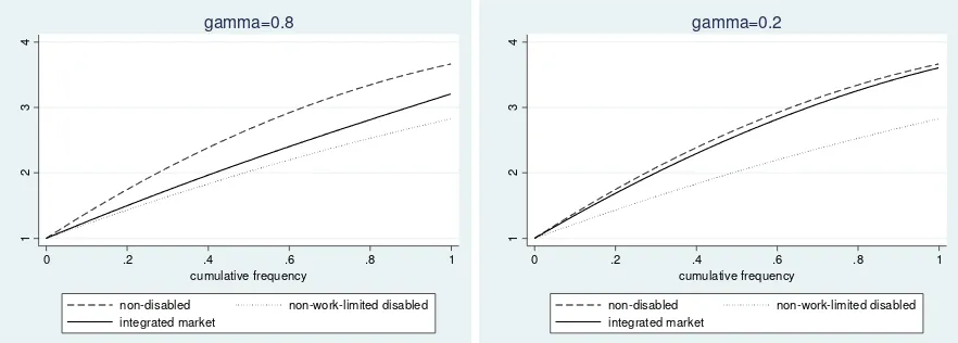
In the discriminatory scenario the wage distribution for the non-disabled is shown by the dashed line whereas for the non-work-limited disabled by the dotted line (see Figure 1). In the non-discriminatory scenario, the wage distribution for the integrated market is shown by the solid line and lies between the two distributions in the discriminatory case. When 0.8 (i.e. 80% of the workers are non-work-limited disabled), the wages of the non-disabled fall substantially if discrimination is not allowed whereas the wages of the non-work-limited disabled slightly increase (left part of Figure 1). The opposite happens if the number of non-work-limited disabled workers is small ( 0.2) – see right part of Figure 1.
It is important to note however, that overall in the non-discriminatory case the wage distribution for the non-work-limited disabled improves but worsens for the non-disabled supporting the model’s main prediction. The magnitude of these changes is different depending on the parameter but can be intuitively explained. For example, when there is a small number of non-work-limited disabled workers in the labour market – which is closer to what happens in reality – the changes in non-discrimination will be bigger to the wages of the underrepresented workers, and most likely being discriminated before in the labour market (i.e. non-work-limited disabled in this case).
3The proofs of these predictions are in the Appendix.
4For the results when destruction rates are different between the non-disabled and non-work-limited disabled see
Figure 1: Wage distributions in the discriminatory and non-discriminatory case – simulated data
3. Concluding remarks
The paper aims to explain any wage differences between the non-work-limited disabled and non-disabled using the monopsonistic approach. If employers are not allowed to discriminate by law against this specific group of disabled we propose an extension of the simple B-M (1998) model of monopsony to account for this case. The models’ main prediction that non -discrimination improves the wage distribution for the non-work-limited disabled but worsens it for the non-disabled is supported by the results from a simple simulation exercise. We should acknowledge however, that in this paper we do not control for business cycle conditions or economic growth.
The models presented in this paper can be used, not only to explain labour market discrimination and non-discrimination on different grounds (for example race, age and sexual orientation), but also to examine the effectiveness of relative anti-discrimination legislation. Future work can consider using real survey or administrative data to assess such effectiveness.
Appendix
Comparative statics
In equilibrium, the wage offer distribution is
b p
w p k
k w
F( ) 1 1 and differentiating
this with respect to k gives
0 1
1
2
b p
w p
k (A1)
Then, it is easy to see that the higher the k the higher the probability of receiving a higher offer 1F(w).
Similarly, the current wage distribution is
1 1
) (
w p
b p k w
G which differentiating
with respect to k gives
1
2
3
4
0 .2 .4 .6 .8 1 cumulative frequency
non-disabled non-work-limited disabled integrated market
gamma=0.8
1
2
3
4
0 .2 .4 .6 .8 1 cumulative frequency
non-disabled non-work-limited disabled integrated market
0 1 1 2 w p b p k (A2)
and therefore, the higher the k the higher the probability of earning a higher wage 1G(w).
Proofs of models’ predictions
Prediction P1
It comes from the fact that kN kD.
Prediction P2
From (P1) and since G is a monotonic transformation of F, it can be easily seen that )
( )
(w G w GN D .
Prediction P3 If
D N i i i i i i k k , ˆ ,
ˆi 0 i, is the proportion of the workers the firm will recruit at a givenwage w in the non-discriminatory case (iN,D for the non-disabled and non-work-limited disabled respectively).
We know that ) ( )
(w F w
FN D (A3)
and in equilibrium it should hold that (profit maximization condition)
2 2 ) 1 ( ) ( ))] ( 1 ( 1 [ ) ( i post i k b p w F k w p
. (A4)
Also,
D N i i i D N i post i i k b p w F k w p , 2 , 2 ) 1 ( ˆ ) ( ))] ( 1 ( 1 [ ˆ )
( (A5)
If F (w) FN(w)
post
it should be that Fpost(w)FD(w). Hence,
i ND i D
i D N i post i i w F k w p w F k w p , 2 , 2 ))] ( 1 ( 1 [ ˆ ) ( ))] ( 1 ( 1 [ ˆ ) (
D Ni i ND i
i post i i A k b p w F k w p , , 2 2 ) 4 ( ) 1 ( ˆ ) ( ))] ( 1 ( 1 [ ˆ )
( , which contradicts (A5).
Therefore, it must be that Fpost(w)FN(w) (A6)
Similarly, suppose that Fpost(w)FD(w). Then, it should be that Fpost(w)FN(w).
Hence,
i ND i N
D Ni i ND i
i N post i i N A k b p w F k w p , , 2 2 ) 4 ( ) 1 ( ˆ ) ( ))] ( 1 ( 1 [ ˆ )
( , which contradicts (A5).
Thus, it must be that Fpost(w)FD(w) (A7)
From (A3), (A6) and (A7) we can conclude that FN(w)Fpost(w)FD(w).
Different job destruction rates
We consider the case where non-work-limited disabled are more likely to leave employment compared to their non-disabled counterparts i.e. they have a higher job destruction rate
)
(D N . By relaxing the assumption of common δ the main conclusion of the paper with regards to the wage distribution of the non-disabled and non-work-limited disabled does not change significantly. To see this, recall that one of the key relationships in the model that drives the results is k rather than λ and δ per se.
In the discriminatory scenario, it is easy to show that the equilibrium wage and job offer distributions will have the same form as with common δ.
In order to find the equilibrium wage offer distribution in the non-discriminatory case, we need to set:
2 2 2 2 ) ( ) ( ) ( ) ( ) 1 ( ))] ( 1 ( [ ) ( ))] ( 1 ( [ ) ( ) 1 ( D D D D D N N N N N post D D D D D post N N N N N k b p k k b p k w F k w p k w F k w p k (A8)
which simplifies to
2 2 2 2 ) 1 ( ) ( ) 1 ( ) ( ) 1 ( ))] ( 1 ( 1 [ ) ( ))] ( 1 ( 1 [ ) ( ) 1 ( D D D N N N post D D D post N N N k b p k k b p k w F k w p k w F k w p k (A9)
In equilibrium, the offer wages (for Fpost(w)1) should lie in the interval:
(p b)
N M p w
b (A10)
with
D D N N k k M
1 and
2
21 1 1 D D D N N N k k k k N .
Results from a simulation exercise for this case are also reported below. We consider a random sample of 1,000 individuals and we examine different values of γ ( 0.8 and
2 . 0
Figure A1: Wage distributions in the discriminatory and non-discriminatory case – simulated data with different job destruction rates
References
Baldwin, M. and W. Johnson (2000) “Labor market discrimination against men with disabilities in the year of the ADA”Southern Economic Journal66, 548-566.
Baldwin, M. and W. Johnson (1994) “Labor market discrimination against men with disabilities”Journal of Human Resources29, 1-29.
Baldwin, M. and E. Schumacher (2002) “A note on job mobility among workers with disabilities”Industrial Relations41, 430-441.
Barth, E. and H. Dale-Olsen (2009) “Monopsonistic discrimination, work turnover and the gender wage gap”Labour Economics16, 589-597.
Becker, G. (1993) Human Capital: a Theoretical and Empirical Analysis, with Special Reference to Education, University of Chicago Press (3rd edition).
Becker, G. (1971) The economics of discrimination, University of Chicago Press (2nd edition).
Burdett, K. and D. Mortensen (1998) “Wage differentials, employer size, and unemployment”International Economic Review39, 257-273.
DeLeire, T. (2001) “Changes in wage discrimination against people with disabilities: 1984-1993”The Journal of Human Resources36, 144-158.
Hirsch, B., T. Schank and C. Schnabel (2010) “Differences in labor supply to monopsonistic firms and the gender pay gap: an empirical analysis using linked employer-employee data from Germany”Journal of Labor Economics28, 291-330.
Johnson, W. and J. Lambrinos (1985) “Wage discrimination against handicapped men and women”The Journal of Human Resources20, 264-277.
Jones, M. (2009) “Disability, employment and earnings: an examination of heterogeneity” Applied Economics43, 1001-1017.
1
2
3
4
0 .2 .4 .6 .8 1 cumulative frequency
non-disabled non-work-limited disabled integrated market
gamma=0.8
1
2
3
4
0 .2 .4 .6 .8 1 cumulative frequency
non-disabled non-work-limited disabled integrated market
Jones, M. (2008) “Disability and the labour market: a review of the empirical evidence” Journal of Economics Studies35, 405-424.
Jones, M. and P. Latreille (2011) “Disability and self-employment: evidence for the UK” Applied Economics43, 4161-4178.
Jones, M. and P. Latreille (2009) “Disability and earnings: Are employer characteristics important?”Economic Letters106, 191-194.
Malo, M. and R. Pagan (2012) “Wage differentials and disability across Europe: Discrimination and/or lower productivity?”International Labour Review151, 43-60.
Manning, A. (2003) Monopsony in Motion, Princeton University Press.
Phelps, E. S. (1972) “The statistical theory of racism and sexism” American Economic Review62, 659-661.
Ransom, M. and R. Oaxaca (2010) “New market power models and sex differences in pay” Journal of Labor Economics28, 267-289.