Mini Squeezers Towards Integrated Systems

A thesis submitted for the degree of Doctor of

Philosophy in Physics

Mini Squeezers Towards Integrated

Systems

Alexandre Brieussel

May, 2016

Australian National University

&

Université Pierre et Marie Curie

Supervisors

:

Prof. Claude FABRE

Prof. Nicolas TREPS

Prof. Ping Koy LAM

Dr. Thomas SYMUL

Declaration

This thesis is an account of research undertaken between October 2011 and January 2016 at The Department of Quantum Science, Research School of Physics, Fac-ulty of Science, The Australian National University, Canberra, Australia and the Laboratoire Kastler Brossel, Paris, France.

Except where acknowledged in the customary manner, the material presented in this thesis is, to the best of my knowledge, original and has not been submitted in whole or part for a degree in any university.

Acknowledgments

First I wish to thanks my official supervisors which were of great help during this thesis. Ping Koy Lam, Thomas Symul in Australia and Claude Fabre and Nicolas Treps in France, but Also my non official supervisors Jiri Janousek and Ben Buchler who were always here to answer my questions and to help me in the lab.

I want to thanks my lab team in Australia who struggled with me with the SqOPO, Shen Yong, Geoff Campbell and my house-mate Giovanni Guccione. I thank all my lab co-workers in Australia hoping not to forget anyone. Sara Hosseini, Jiao Geng, Syed M Assad, Helen Chrzanowski, Seiji Armstrong, Sophie Zhao Jie, Oliver Thearle, Jin Yang, Melanie Mraz and Mark Bradshaw, and the people I didn’t necessary worked with, but with who I shared meals, played cards or that I just met in the corridor and had a chat Pierre Vernaz-Gris, Harry Slatyer, Mahdi Hosseini, Daniel Higginbottom, Julien Bernu, Jesse Everett, Jian Su, Boris Hage, Jessica Eastman, Shasha Ma, Young-Wook Cho, Ben Sparkes and André Carvalho from the group and Michael Stefszky, Georgia Mansell, John Debs with his 3D printer, Nick Robin and Kyle Hardman that I always met late in the week-end and John Close who teached me how to play guitar. In France I also want to thanks my lab coworkers Hanna Lejeannic, Guillaume Labroille, Olivier Morin, Kun Huang, and Julien Laurat. And the people in my group Pu Jian, Jean-François Morizur, Valérian Thiel, Clement Jacquard, Valentin A. Averchenko, Roman Schmeissner, Jonathan Roslund, Vanessa Chille, Cai Yin, Guilia Ferrini, Zheng Zhan and also Simon François, Baptiste Gouraud, Dominik Maxein, Leander Hohmann, Sebastien Garcia, Konstantin Ott, Claire Lebouteiller and Jacob Reichel.

Abstract

Squeezed states of light are quantum states that can be used in numerous protocols for quantum computation and quantum communication. Their generation in labora-tories has been investigated before, but they still lack compactness and practicality to easily integrate them into larger experiments.

This thesis considers two experiments: one conducted in France, the miniOPO; and one conducted in Australia, the SquOPO. Both are new designs of compact sources of squeezed states of light towards an integrated system.

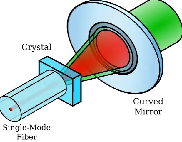
The miniOPO is a linear cavity of 5mm length between the end of a fiber and a curved mirror with a PPKTP crystal of 1mm inside it. The squeezing generated in this cavity is coupled into the fiber to be able to be brought to a measurement device (homodyne) or to a larger experiment. The cavity is resonant for the squeezed light and the pump light, and locked in frequency using self-locking effects due to absorption of the pump in the crystal. The double resonance is achieved by changing the temperature of the crystal.

Two different fibers have been tested in this experiment, a standard single-mode fiber and a photonic large core single-mode fiber.

The squeezing obtained is still quite low (0.5dB with the standard fiber and 0.9dB

for the photonic fiber) but a number of ameliorations are investigated to increase these levels in the future.

The SqOPO is a monolithic square cavity made in a Lithium Niobate crystal using four total internal reflections on the four faces of the square to define an optical mode for the squeezed mode and the pump mode. The light is coupled in the resonator using frustrated internal reflection with prisms. The distance between the prisms and the resonator defined the coupling of the light, which allows us to control the finesse of the light in the resonator and by using birefringent prisms it is possible to tune independently the two frequencies in the resonator to achieve an optimal regime. The frequency of the light is locked using absorption of the pump light in the resonator to achieve self-locking, and double resonance is controlled by tuning the temperature of the crystal.

We demonstrated 2.6dB of vacuum squeezing with this system. Once again, the

Publication:

Contents

Acknowledgments 5

Abstract 7

I.

Theoretical Background

1

1. Introduction 5

1.1. The Maxwell Equations and the Wave Equations . . . 5

1.2. Energy Considerations . . . 6

1.3. Fourier Transforms . . . 6

1.4. Dielectric Medium and the Wave Equation . . . 8

1.4.1. Properties of Susceptibilities . . . 8

2. Light Propagation 11 2.1. Linear Homogeneous Isotropic (LHI) Behavior . . . 11

2.1.1. Gaussian Propagation Solution . . . 12

2.1.2. High Order Propagation Mode Solutions . . . 13

2.1.3. Astigmatism . . . 14

2.1.4. ABCD Matrix . . . 14

2.2. Linear Anisotropic Medium . . . 15

2.2.1. Ordinary Beam . . . 18

2.2.2. Extraordinary Beam . . . 19

2.2.3. Dispersion Angle . . . 19

2.3. Non Linear Medium . . . 20

2.3.1. Propagation Equation . . . 20

2.3.2. Second Harmonic Generation . . . 22

2.3.3. Degenerate Parametric Amplification . . . 24

3. Interface Conditions 25 3.1. Field Interface Conditions . . . 25

3.1.1. Normal Fields . . . 25

3.1.2. Tangential Fields . . . 26

3.1.3. Poynting Vector . . . 26

3.2. Fresnel Equations . . . 26

3.2.1. TE Polarization or S-Polarization . . . 28

4. Cavity 33

4.1. Beam Splitter Conventions . . . 34

4.2. Cavity Transmission . . . 34

4.3. Stability . . . 37

4.4. Non Linear Cavity . . . 39

5. Quantum Optics 43 5.1. Quantization of the Field . . . 43

5.2. Quadratures and Homodyne Measurements . . . 46

5.2.1. Quadratures . . . 46

5.2.2. Optics Components . . . 46

5.2.3. Homodyne . . . 47

5.3. Different Light States and Wigner Function . . . 49

5.3.1. Fock States . . . 50

5.3.2. Coherent States . . . 51

5.3.3. Squeezed States . . . 52

5.4. Squeezing Creation and Interaction with Environment . . . 53

5.4.1. Single pass squeezing generation in a non-linear crystal . . . . 53

5.4.2. Squeezing Interaction in a Lossy Channel . . . 55

5.4.3. Squeezing generation in a non linear crystal in a cavity . . . . 55

II. Fibered Mini OPO

61

6.2. Squeezing Generation . . . 63

6.3. Toward an all-fibered squeezer . . . 64

7. Experimental Method 67 7.1. The OPO Cavity, Description of the Experiment . . . 67

7.1.1. Coupling Mirror . . . 68

7.1.2. Crystal and Crystal Mount . . . 71

7.1.3. Fiber and Fiber Mount . . . 73

7.1.4. Base . . . 75

7.2. Other experimental consideration . . . 75

7.2.1. Laser Source . . . 75

7.2.2. Fibered Elements . . . 76

7.2.3. Crystal Temperature Control . . . 80

7.2.4. High Voltages Amplifiers: . . . 81

7.2.5. Homodyne Detectors . . . 81

7.2.6. Optical Suspension Table . . . 83

7.3. Alignment of the Cavity . . . 83

7.3.1. Schematic of the Set Up . . . 83

7.3.2. Crystal Alignment with White Light Interferometry . . . 84

7.3.3. Temperature Tuning . . . 87

7.3.4. Homodyne Alignment: . . . 87

7.3.5. Curved Mirror: . . . 89

7.3.6. Alignment of the Green and Red: . . . 90

7.4. System Limitations . . . 91

7.4.1. Curvature Matching . . . 91

7.4.2. Asphericity of the phase surfaces . . . 92

7.4.3. Grey Tracking and Damaging: . . . 95

7.5. Locking the System . . . 96

7.5.1. PDH locking . . . 96

7.5.2. Self Locking . . . 97

7.5.3. Locking with a Micro-Controller . . . 100

8. Results 103 8.1. Second Harmonic Generation and Amplification De-Amplification . . 103

8.2. Squeezing . . . 104

9. Conclusion 109

III. Square Monolithic Resonator

115

11.1.1. S-Polarization . . . 122

11.1.2. P-Polarization . . . 124

11.2. Resonator . . . 126

11.3. Phase Control . . . 130

11.4. TEM Modes . . . 132

11.5. ABCD Matrix Considerations and Stability of the resonator . . . 132

12.Experimental Methods 135 12.1. Creation of Resonators . . . 135

12.1.1. Polishing . . . 135

12.2. Prisms . . . 136

12.3. Mechanical System . . . 137

12.4. High Voltage . . . 141

12.5. Alignment . . . 141

12.5.1. How to Align Prisms and Resonators . . . 141

12.5.2. How to Align the Beam with Contra-Propagating Beams . . . 143

12.5.4. Homodyne Alignment . . . 145

12.5.5. Prism Switching and alignment for Squeezing . . . 146

12.6. Lock and Self Locking . . . 147

13.Results 151 13.1. Non Linearity . . . 151

13.1.1. SHG and De-amplification . . . 151

13.1.2. Squeezing . . . 151

13.1.3. Conclusion . . . 154

A. Fourier Transform of the Polarisation Field versus the Susceptibility 161 B. Index calculation for the green calcite coupler in p-polarization 165

Part I.

Overview of the Thesis

During the last 50 years, we have witnessed the huge development of information technology around the world, to the point where almost everyone now has a computer in their home and an Internet-connected Smartphone in their pocket. One of the key points that allowed this sudden development was the progress of the transistors. Quantum computation and quantum communication are the future of our informa-tion technology and like the transistor, the source of quantum states used in these technologies will be the key point for their development. Amongst the different me-dia for these states, light is fast, easy to transport and has good interaction with matter. The two simpler candidates for quantum states of light are single photons and squeezed states. A lot of work has been done in the production of single photons, this thesis emphasizes the production of squeezing states.

This Ph.D. was a collaboration between the Laboratoire Kastler Brossel in Paris and the Australian National University in Canberra to investigate two new compact designs to potentially operate as sources of squeezing of light for larger experiments. The first one, the miniOPO, has been developed in Paris. It is a linear cavity between the end of a fiber and a curved mirror containing a non linear crystal of PPKTP. The advantage of this system is the fact that the squeezed light is directly injected in the fiber allowing easy transfer and potential processing to be done directly in the fiber. This system will be presented in the second part of the thesis. The second system considered, the SqOPO, has been developed in Canberra. It is a square piece of crystal of Lithium Niobate acting as a ring cavity with four total internal reflections on the four faces of the square. The coupling with this system is made with frustrated total internal reflection with two prisms brought into the evanescent field of the resonator. This system will be described in the third part.

But because these two systems applied a few advanced concepts of optics, this first part will provide the reader with an introduction to the necessary concepts to understand this thesis. We will start by introducing the notion of general wave propagation, and then apply it to isotropic linear material, to anisotropic material, and to non linear materials. Then we will consider interface behavior and cavities concepts. And finally we will consider the notions of quantum states with squeezed states (Figure 0.1).

Writing Conventions: In this thesis I will be using normal characters for scalar

Chapter 0

Gaussian Beams

ABCD Matrix

Fresnel Equation

Anisotropic Material Non Linearity

Cavities

Squeezing

Figure 0.1.: Schematics of the two systems used in this thesis and all the concepts

used for each one that will be presented in this introduction.

fields like E the electric field and B the magnetic field, I will use bold characters

with an over-line for tensors like the permittivity tensor, and I will use a hat for

operators like the creation operator ˆa†.

I will be using Einstein’s convention of summing terms with repeated indices, I will use the Kronecker tensorδij and I will call the two lights used in this thesis: 1064nm

light red light or sub-harmonic for the light at the wavelength of 1064nm; and 532nm light, green light or pump for the light at the wavelength of 532nm.

1. Introduction

1.1. The Maxwell Equations and the Wave Equations

We start this thesis by enunciating the four Maxwell equations [13]. These describe, the behavior of the electric field, E; the magnetic field,B; the electric displacement

field, D = ε0E+P; and the magnetizing field, H= _µ1₀B. Here, P is the

polariza-tion field due to fixed charges of the material, and ε0 and µ0 are, respectively, the

permittivity and the permeability of free space. The equations are:

Maxwell-Gauss Maxwell-Faraday

∇ ·D =ρf, ∇ ×E=−∂_∂tB,

Maxwell-Thomson Maxwell-Ampère

∇ ·B= 0, ∇ ×H=jf +∂_∂tD,

(1.1)

where jf is the free current density, andρf is the free charge density.

By applying the Curl to the Faraday equation and using the Maxwell-Ampère equation to eliminate the magnetic field in the assumption that there is no free current, i.e. jf = 0, we obtain the wave equation:

∇ ×(∇ ×E) = −∂(∇ ×B)

∂t =−

1

c2

∂2_E

∂2_t −µ0

∂2_P

∂2_t, (1.2)

where c= √1

0µ0 is the speed of light in the vacuum.

By using the expression ∇ ×(∇ ×E) = ∇(∇ ·E)− 4E, we obtain an other form

of the wave equation:

∇(∇ ·E)− 4E=−1

c2

∂2_E

∂2_t −µ0

∂2_P

∂2_t., (1.3)

Chapter 1 Introduction

1.2. Energy Considerations

Consider some free charges {qf,i} moving at speed {vi} in an electromagnetic field

{E,B} in matter. The charges experience a force fi =qi(E+vi∧B), which corre-sponds to a power P =qivi·E. The density of electric power on the free charges is given by:

P =jf ·E

It is the energy held by the free charges in the field.

By using the Maxwell-Ampère equation, the property: ∇·(E×B) = B·(∇ ×E)−

E·(∇ ×B) and Maxwell-Faraday we obtain the Poynting Theorem [16] describing

the electromagnetic energy conservation:

∂u

∂t + div(Π) =−jf.E

Where Π = E×H is the Poynting vector and u = 1₂(E.D+B.H) is the

electro-magnetic energy density.

The change in electromagnetic energy is equal to a flux described by the Poynting vector and a source term given by the energy held by the free charges.

1.3. Fourier Transforms

The Maxwell equations are a bit complicated to use directly, but a good simplifica-tion of them can be achieved by using Fourier transforms. It allows us to solve the field equations in the Fourier domain and come back to the field in the time domain with an inverse transformation. For a fieldE(r, t), and its Fourier transform in time E(r, ω), the two field vectors are related by

E(r, ω) = _π1 R+∞

−∞ E(r, t) exp(iωt)dt and E(r, t) = 12

R+∞

−∞ E(r, ω) exp(−iωt)dω .

(1.4)

In this thesis, the fieldE(r, t) is a real field, soE(r, ω) satisfies the propertyE(r, ω) = E∗(r,−ω). Thanks to this it is possible to restrain ourselves to positive frequency

values and take the real part of the complex field:

E(r, t) = <

Z ∞

0

E(r, ω) exp(−iωt)dω

. (1.5)

1.3 Fourier Transforms

It is also possible to extend the Fourier transform to the spatial coordinate by using the wave vector space k:

E(k, ω) = 1 (2π)3

R

E(r, ω) exp(−ik.r)dr and E(r, ω) =R

E(k, ω) exp(ik.r)dk .

(1.6)

The sign convention is inverted for space and time to make the field with one single positive frequency ω and one single wave vector k propagate in the direction of k.

We call this particular solution a plane wave.

The real field in function of the complete Fourier transform in space and time is given by

E(r, t) =<

Z ∞

0

Z

R3

E(k, ω) exp(−iωt) exp(ik.r)dkdω

(1.7)

where E(k, ω) is the Fourier transform of the field in space and time. It can be seen

as a superposition of waves with a particular distribution E(k, ω). Because of the

linearity of the Maxwell equations, it is possible to only consider propagations of single waves and to add them weighted by the distribution E(k, ω) to obtain the

propagation of the real field. (Eq. 1.7).We can consider the field of a wave to be

E(r, t) =E0exp(−iωt) exp(ik.r) +c.c (1.8)

with E0 the amplitude vector of the wave. In this regime, the Maxwell equations become:

Maxwell-Gauss Maxwell-Faraday k·D=ρf k×E =iωB

Maxwell-Thomson Maxwell-Ampère k·B = 0 k×H =jf −iωD

, (1.9)

and the wave equation (Eq. 1.3) becomes

−(k·E)k= ω

2

c2 −k 2

!

Chapter 1 Introduction

1.4. Dielectric Medium and the Wave Equation

In a dielectric material, without any electric field for a sufficient period of time, the polarization of the material,P, will be equal to zero. The polarization fieldP(r, t) is

a function of the electric field E, but the response is not necessarily instantaneous;

rather, it will depend on every component of E(r, t0) at every value of the time, t0 < t. The Taylor series expansion of the polarization will be given by:

Pi(t) = ε0

R

χ1

ij(t−τ)Ej(τ)dτ

+ε0

RR

χ2

ijk(t−τ1, t−τ2)Ej(τ1)Ek(τ2)dτ1dτ2

+...

+ε0RRRR χNij1...jN(t−τ1, ..., t−τN)Ej1(τ1)...EjN(τN)dτ1dτ2...dτN +...

,

withχN

ij1...jN representing the susceptibility of orderN, a tensor of orderN+ 1 with each coefficient a function of N + 1 variables corresponding to the dependence in

time of each electric component in the decomposition. For the purpose of this thesis, we will restrain ourselves to the two first terms of the decomposition, χ1

ij(t1) and

χ2_ijk(t1, t2).

In the Fourier domain, we obtain:

Pi(ω) = ε0χ1ij(ω)Ej(ω) +ε0

Z

χ2_ijk(ω0, ω−ω0)Ej(ω0)Ek(ω−ω0))dω0. (1.11)

The demonstration of this calculation is given in Appendix A.

1.4.1. Properties of Susceptibilities

The susceptibility coefficients have to satisfy some symmetry conditions that con-strain their values. First, the polarization vector and the field vectors are real vectors, meaning that the quantitiesχN

ij(t1, ..., tN) also have to be real. The Fourier

transforms of the first two orders must satisfy

χ1

ij(ω) = χ1ij(−ω)∗,

χ2_ijk(ω1, ω2) = χijk2 (−ω1,−ω2)∗.

A second property of the second order susceptibility is obtained from intrinsic sym-metry. It corresponds to the fact that it doesn’t matter which field is the first and which one is the second in Eq. 1.11, it gives:

1.4 Dielectric Medium and the Wave Equation

χ2_ijk(ω1, ω2) =χ2ikj(ω2, ω1).

This particularity of the notation can cause some confusion. If the two frequencies considered are equal, we will get P(2ω) = χ2_ijk(ω, ω)E2(ω), but if the frequencies

are not equal, we will obtain P(ω1 +ω2) = 2χ2ijk(ω1, ω2)E(ω1)E(ω2). The factor

two comes from the possibility of writing E(ω1)E(ω2) as E(ω2)E(ω1) in equation

(Eq. 1.11).

If the material is considered lossless (which we will suppose for the rest of this calculation) then the first and second order coefficients of the susceptibility need to be real:

χ1

ij(ω) = χ1ij(ω)

∗ _χ2

ijk(ω1, ω2) = χijk2 (ω1, ω2)∗ .

There also exist two other symmetry conditions due to the fact that the material is considered to be lossless. It implies that the first order susceptibility is a symmetric tensor,

χ1_ij(ω) =χ1_ji(ω),

and that we can permute the frequencies and the coefficients of the second order susceptibility:

χ2_ijk(ω1, ω2) =χ2jik(ω1+ω2,−ω2) =χ2kij(ω1+ω2,−ω1). (1.12)

2. Light Propagation

2.1. Linear Homogeneous Isotropic (LHI) Behavior

To give the basics of wave propagation, we will first consider the LHI model. This means that we consider a susceptibility which is constant in the medium and given only by the first order in the applied electric field (χ(N) _{= 0 forN ≥2). Moreover,}

we suppose the response of the material to be the same in each direction. This means that χ(1) is a scalar.

Pi(ω) = ε0χ(ω)Ei(ω). (2.1)

Maxwell-Gauss equation implies that ∇ · E = 0 in Eq. 1.3, so by expressing the

refractive index of the material as n =q(1 +χ) we get the LHI wave propagation

equation:

4E= n

2

c2

∂2_E

∂2_t. (2.2)

Applying this equation to a single plane wave of frequency ω and wave vector k,

one obtains the expression:

k2 =n2ω

2

c2

Moreover, we have ∇ ·E = k·E = 0, implying that the vector E is orthogonal to

the vector k. It is possible to define two vectors1(k) and 2(k) orthogonal tokas

a basis for the direction of the electric field.

To characterize the usual coherent beams in free space, we will suppose the light propagating along ez, and we will suppose the electric field to be a plane wave with

an amplitude slowly varying with the position:

E(x, y, z, t) = X

i=(1,2)

Chapter 2 Light Propagation

By using the propagation equation Eq. 2.2 and by supposing

∂2_E

i ∂z2 k

∂Ei ∂z

, which

means that the variation ofEi inz is negligible within the scale of a wavelength, we

obtain the paraxial Helmholtz propagation equation for Ei:

∂2_E i

∂x2 +

∂2_E i

∂y2 + 2ik

∂Ei

∂z = 0 (2.3)

By transforming the x and y coordinates ofEi to the Fourier domain, we get:

−(k2_x+k_y2)Ei(kx, ky, z) + 2ik

∂Ei(kx, ky, z)

∂z = 0

We obtain a solution in the shape:

Ei(kx, ky, z) = Ei(kx, ky,0)e−i k2_x+k_y2

2k z (2.4)

More details about propagation solutions for light can be found in [2].

2.1.1. Gaussian Propagation Solution

If we start in the plane at z = 0 with a field of Gaussian distribution Ei(x, y,0) =

q

2 π

E0

w0e

−x2+y2

w2

0 wherew2

0 is the variance of this distribution, andE0, the amplitude of

this distribution (R

|Ei(x, y,0)|2dxdy =|E0|2).

The Fourier distribution of this function isEi(kx, ky,0) =

√

2πw0E0e− k2_x+k2_y

4 w02. Using Eq. 2.4 and using the inverse Fourier transform we obtain the expression of the Gaussian beam field:

E

(

x, y, z

) =

k

E

√

2

π

w

iq

(

z

)

e

ikx₂2+_q(zy₎2

with q(z) =z−izR and zR= kw2

0

2 the Rayleigh’s range.

This Gaussian beam has a waist size in z given by

w(z) = w0

s

1 + z

zR

2

2.1 Linear Homogeneous Isotropic (LHI) Behavior

The curvature radius of the beam is given by

R(z) =z+z

2 R

z ,

and the phase shift that the beam is experienced in function of z is:

ψ(z) = arctan( z zR

).

The coefficient q can be expressed in function of the waist and the curvature by:

1

q(z) =

1

R(z)+i

2

kw2. (2.5)

2.1.2. High Order Propagation Mode Solutions

In the same way it is possible to propagate a beam given by a Gaussian beam weighted by Hermite polynomials:

Ei,nm(x, y,0) =E0

√

21−n−m

w0

√

πm!n!Hn( x√2

w0 )

Hm(

y√2 w0 )

e−

x2+y2 w2

0

with Hn the Hermite polynomial given by: Hn(ξ) = (−1)neξ

2 _dn dxne

−ξ2 . Fields having this expression can be seen to be orthogonal: R

Ei,nm(x, y,0)Ei,kl(x, y,0)dxdy=

|E0|2δnkδml. Adding the propagation in the z direction, the field mode reads

Ei,nm(x, y, z) =E0

√

21−n−m

w(z)√πm!n!Hn( x√2 w(z))Hm(

y√2 w(z))e

ik(x₂2+_q(zy₎2)−iψnm(z)+ikz _(2.6)

with a generalized phase shift ψnm(z) = (1 +n+m) arctan(_zz R).

The family of functions n

unm(x, y, z) =

Ei,nm(x,y,z)

E0

o

nm constitutes an orthonormal

basis of solution of Eq. 2.3 (R

|unm|2dxdy = 1 and

R

|unmukldxdy = δnkδml). That

Chapter 2 Light Propagation

a

b

c

d

e

x

y xy xy xy xy

x

z

f

Figure 2.1.: (a) to (e) are transverse Hermitian mode intensities (from left to right

TEM00, TEM10, TEM01, TEM11 and TEM02). f) is the intensity projection of a Gaussian beam in a plane containing the propagation axis.

2.1.3. Astigmatism

In the development of Gaussian beams and higher-order modes we supposed a dis-tribution identical in the directionsexand ey. But it wasn’t necessary, it is possible to separate the problem in the direction x and y , The electric field becomes

Ei(x, y, z) =E0u(x)n (x, z).u (y) m (y, z)

with u(i)

n such that

R∞

−∞u(i)n (ξ, z)u(i)

∗

m (ξ, z)dξ=δnm given by:

u(i)_n (ξ, z) = Hn(

√

2ξ wi(z))e

ikξ2

2_qi(z)

r

wi(z)

q_π

22 n_n!

This decomposition has the same generality than Eq. 2.6, but because it allows to consider modes with different waist size and positions in the direction x and y, it

can be more convenient to use in a cavity with non spherical mirrors .

2.1.4. ABCD Matrix

The ABCD matrix method is a convenient way to propagate the light through an optical system based on a ray tracing matrices. The beams of light before and after this system are characterized by two parameters: the distance from the optical axis (xi and xo); and the angle relative to this axis (θi and θo). The optical system

is considered as a two dimensional matrix M = A B

C D

!

corresponding to the transformation of the two parameters (Figure 2.2).

xo

θo

!

= A B_{C D}

!

xi

θi

!

2.2 Linear Anisotropic Medium

( )

x

θ

θ

x

Optical

System

Incident

ray

Transmitted

ray

Optical

Axis

Figure 2.2.: An optical system is analyzed by the transfer matrix between the

distance from the optical axis and the angle with the optical axis at the entry of the system (xi, θi) and the same parameters at the output of the system (xo, θo).

M has to satisfy Det(M) = n1

n2 withn1 and n2 the indices of the medium before and after the considered optical system.

The ABCD matrices are interesting because they can also be used for propagation of a Gaussian mode, where instead of the pair of parameters (x, θ), the complex

parameter q(z) (Eq. 2.5) is used:

qo =

Aqi+B

Cqi+D

. (2.7)

ABCD matrices of several sub-systemsT1...Tncrossed by the beam can be combined

together so that they can be considered as a single, bigger system.

Ttotal=Tn∗...∗T1.

Table 2.1 presents some of the most common matrices used in this thesis.

As we will see in the section on resonators (section 4.3), in order to have a beam resonating in a cavity, it needs to be identical to itself after a full round trip. There-fore, the ABCD matrix of a round trip applied to the q parameter of a mode needs

to give the same value q. More details will be given in the section on cavities

(section 4.3). The reader can access more detail on Gaussian beams and ABCD matrices in references [15] and [9].

2.2. Linear Anisotropic Medium

In this part, we will consider a linear material, which means: χ(2) = 0, but this

Chapter 2 Light Propagation

Matrix Elements

1 d

0 1

!

Propagation in a medium for a distance d.

1 0

−2/Re 1

! Reflection at a curved

mirror with an angle θ with

the normal.

g(α) 0

0 n1

n2

1 g(α)

! Refraction at a flat surface

between two indices n1 and

n2 with an angle α with

the normal.

Table 2.1.: ABCD matrices used in this thesis. Re = Rcos(θ) in the tangential

plane (horizontal direction), Re =R/cos(θ) in the sagittal plane (vertical

direc-tion). For the refraction, g(α) =

v u u

t1−

n₁ n₂sin(α)

2

cos2_(α) whereα is the angle between the beam and the normal to the surface.

superscript in the following). The polarization in this birefringent material can be expressed as::

Pi(ω) = ε0χij(ω)Ej(ω)

We usually use the relative permittivity: ij =δij +χij(ω), to describe the relation

between the electric displacement and the electric fieldD =ε0εE.

The susceptibility is symmetric, so the permeability is also symmetric. There exists a basis where the matrix ij is diagonal.

ε=



 

εx 0 0

0 εy 0

0 0 εz



 

Where εi, i ∈ {x, y, z} are the eigenvalues of ε. By analogy with the isotropic

case, we get three refractive indices ni =

√

i . If all three of the values are equal

nx = ny = nz, it corresponds to the isotropic case; if only two of them are equal,

the material is called uniaxial; and if the all of them are different, it is a biaxial material. In the case of this thesis we will always consider uniaxial birefringence (nx =ne and ny =nz =no) .

The Maxwell-Gauss ∇ ·D = 0 and Maxwell-Thomson ∇ ·H = 0 equations imply

that the two fieldsD and Hare orthogonal to the wave vector k.

2.2 Linear Anisotropic Medium

k·D= 0 k·H= 0

Note that in this case: ∇ ·E 6= 0, the electric field is not necessarily perpendicular

to the wave vector.

By returning to the propagation equation Eq. 1.10, and by using the expression of the polarization in function of the electric field E and the relative permittivity ε,

we obtain:

Ek2−(k·E)k−ω

2

c2εE = 0 (2.8)

One way to deduce the anisotropic Fresnel equation from there is to rewrite Eq. 2.8 for the three components of the electric field as a function of the components of the wave vector in the basis where εij is diagonal. The propagation equation reduces to

a matrix equation: A(k, ω)E = 0 with A given by:

A(k, ω) =



  

ω2

c2n2x−ky2−k2z kxky kxkz

kykx ω

2

c2n

2

y−k2x−kz2 kykz

kzkx kzky ω

2

c2n

2

z−kx2−ky2



  

. (2.9)

For a non-trivial solution for the electric field to exists, the determinant of this matrix needs to be zero, Det(A) = 0. In this way, after a bit of calculation, we can

obtain the Fresnel anisotropic equation. Another more elegant way to obtain the Fresnel anisotropic equation is to write the electric field Ei in the basis where εij is

diagonal as a function of k·E:

Ei = (

k·E)ki

k2₋ω2

c2n2i

(2.10)

Multiplying the left and right sides of Eq. 2.10 by ki and summing up in terms of i,

we get:

(k·E) = X

i

(k·E)k2 i

k2₋ω2

c2n2i

(2.11)

By simplifying byk·Eand since{ki}verify 1 = _k12

P

iki2, we get the Fresnel equation:

n2_xk2_x

_k

k0

2

−n2 x

+ n2yky2

_k

k0

2

−n2 y

+ n2zkz2

_k

k0

2

−n2 z

Chapter 2 Light Propagation

with k0 = ω_c.

If we put these three terms in the same denominator and restrict ourselves to an uniaxial material: nx =ne and ny =nz =no, we obtain

n2_ek_x2





k k0

!2

−n2_o

    k k0 !2

−n2_o



+n2_o

k_y2+k2_z





k k0

!2

−n2_e

    k k0 !2

−n2_o



 = 0.

(2.13)

Eq. 2.13 has two solutions fork, the first one is given byk2 _=n2

ok02, with no constrain

yet on the direction. It is the ordinary beam wave vector. The second one is obtained by simplifying Eq. 2.13 by_k

k0

2

−n2 o

and by noticing that the coefficient in _k

k0

2

in the new equation is n2 o

k2

y +k2z+kz2

= n2

ok2. we

obtain:

k2 x

n2 o

+ky2+k2z

n2 e

=k₀2 (2.14)

which is the equation obeyed by the extraordinary beam wave vector.

If the wave vector is real and its components satisfy: kx=nk0cos(θ) andky and kz

such that: k2

y+k2z =nk0sin(θ) withnthe index that this field experiences and θthe

angle between the wave vector and the extraordinary axis of the crystal, Eq. 2.14 become the regular expression from text books giving n in function of θ:

cos2(_θ)

n2 o

+ sin2(θ)

n2 e

= 1

n2

2.2.1. Ordinary Beam

In directionej where j ∈ {x, y}such as k2−ω 2

c2n2_j 6= 0 we derive from Eq. 2.10 that: (k·E) = 0

The ordinary beam is orthogonal to the wave vector Eo⊥k. Similarly, supposing that n 6= no, so k2 − ω

2

c2n2o 6= 0, Eq. 2.10 in direction ex also shows that Ex = 0,

so the ordinary polarization is also perpendicular to the extraordinary axis Eo⊥ex. We obtain

2.2 Linear Anisotropic Medium

Eo ∼



 

0

kz

−ky





.

We have also Do = ε0n2oEo, and the Poynting vector Π = E×H parallel to the wave vector: Πkk.

2.2.2. Extraordinary Beam

The electric displacement is perpendicular to the wave vector De·k=Do·k= 0, and the extraordinary beam and the ordinary beam are orthogonal polarizations:

De ·Do = 0. Since the Fresnel equation Eq. 2.12 can be interpreted as a scalar product of the wave vectorkand a vectord= n2ekx

k k₀

2

−n2

e

ex+ n 2 oky k k₀ 2

−n2

o

ey+ n 2 okz k k₀ 2

−n2

o

ez , d·k= 0, and we can notice that d⊥Do, we obtain that De is parallel tod:

De∼

          n2 ekx k k₀ 2

−n2

e n2oky

k k₀

2

−n2

o n2okz

k k0

2

−n2

o           .

Knowing that E= ε_ε−1

0 D, we get:

Ee∼ 1 ε0          kx k k0 2

−n2

e ky k k₀ 2

−n2

o kz k k0 2

−n2

o          .

2.2.3. Dispersion Angle

It can be useful to know the angle between the electric field Eand the displacement

field D. This angle is also the angle between the Poynting vector and the wave

vector:

tan(α) = |Ee×De| Ee·De =

(n2 o−n2e)

n2 e+n2o

_k2

y+k2z k2

x

q

k2 y +k2z

kx

Chapter 2 Light Propagation

2.3. Non Linear Medium

2.3.1. Propagation Equation

In this section, we will consider nonlinear material χ2 6= 0, but for the sake of

simplicity, we will consider the linear susceptibility to be a scalar χ1

ij = χ1δij to

avoid the problems of birefringence. In practice, it will not be true, but as long as we consider only polarizations of the beams in the axis of the crystal, it is good enough to consider the index of this specific polarization direction and to momentarily pretend the case to be isotropic. We return to the wave equation of propagation from the introduction:

∇(∇ ·E(r, t))− 4E(r, t) =−1

c2

∂2E(r, t) ∂2_t −µ0

∂2P(r, t)

∂2_t , (2.15)

In most literatures, the first term is neglected. It is equivalent to neglect the con-tribution of the non-orthogonal field to the wave vector which is usually very small. Taking the Fourier Transform in time of Eq. 2.15 and decomposing the polarization into linear and non linear terms: P=P(1)+_P(2), we obtain:

4E(r, ω) = −ω

2

c2E(r, ω)−µ0ω

2_(P1_{(r, ω) +P}2_{(r, ω)),}

We can get rid of the linear term of the polarization by considering the linear permit-tivity of the material =n2. We can project the equation on a basis orthogonal to

the direction of the field Econsidered and use the non linear susceptibility. We can

simplify the non linear polarization in Eq. 1.11 by considering only three frequencies

ω1,ω2 and ω3 =ω1+ω2, and only one polarization at each frequency. We need only

to consider the component of the second order susceptibility which links these three frequencies together. We will express this as def f. The non linear polarization is

given by:

P(2)(ω) =ε0def fE(ω1)E(ω2) (2.16)

The propagation equation Eq. 1.3 becomes:

4E(r, ωi) =−

ω2

c2n(ωi)E(r, ωi)−µ0ω

2_P(2)_{(r, ω} i).

In the same way as in linear optics Eq. 2.1, we consider the propagation of the beam mostly in the direction ez, and the field to have the shape:

E(ωi, x, y, z) = E(ωi, x, y, z)eikiz

2.3 Non Linear Medium

Where E(ωi, x, y, z) is the slowly varying amplitude. It means k2i = ω

2

c2n(ωi).

The paraxial approximation,

∂2_E

∂z2 k ∂E ∂z

, gives the paraxial non linear equation:

∆⊥E(ωi,r⊥, z) + 2iki

∂E(ωi,r⊥, z)

∂z =−ω

2

iµ0P(2)(ωi,r⊥, z)e−ikiz (2.17)

Where ∆⊥ = ∂

2

∂x2 +

∂2

∂y2. and r⊥ =xex+yey.

To obtain a general solution, we can use the solutions of the paraxial Helmholtz equation : ∆⊥uinm(r⊥, z) + 2iki∂u

i nm(r⊥,z)

∂z = 0 where u

i

nm(r⊥, z) forms a set of

or-thonormal basis by satisfying: RR

dxdyui∗

nm(r⊥, z)uipl(r⊥, z) = δnpδml, and use the

decomposition of the electric field in this basis:

E(ωi,r⊥, z) =

X

lm

Ai_lm(z)ui_lm(r⊥, z)

where Ai

lm(z) is the amplitude of the electric field on the mode (l, m).

However, for the purposes of this thesis, we will restrain ourselves to Gaussian beams with a waist in z = 0, so

ui(r⊥, z) =ui₀₀(r⊥, z) =

s

kizRi

π ∗ i

q(z)exp i

"

kir2

2q(z)

#!

,

where q(z) = z−izRi and zRi is the Rayleigh length of the beam.

The electric field is given by:

E(ωi,r⊥, z) =Ai(z)ui(r⊥, z)

The paraxial equation Eq. 2.17 becomes:

∂Ai(z) ∂z =i

ω_i2µ0

2ki

ZZ

dxdyui∗(r⊥, z)P(2)(r, z, ωi)e−ikiz. (2.18)

By substituting the non linear polarization term in Eq. 2.18 for Eq. 2.16, and by considering ω1 = ω2 = ω, we get a system of two coupling equations for Aω, the

field at frequency ω, and A2ω, the field at the frequency 2ω.







∂Aω_(z)

∂z = i

ω

2nωcdef fΛ(z)A

2ω_(z)Aω∗_(z)e−i∆kz ∂A2ω_(z)

∂z = i

ω

n2ωcdef fΛ(z)

Chapter 2 Light Propagation

where Λ(z) = RR

dxdyu2ω(r, z)uω(r, z)∗uω(r, z)∗,∆k = 2kω −k2ω; nω and n2ω the

refractive indices of beams at frequenciesω and 2ω.

We have nω ≈ n2ω = n which makes k2ω ≈ 2kω . We also consider the Rayleigh

length of the beam at frequencies 2ω and ω to be equal . We denote it zR. (In

practice, we consider only doubly resonant OPOs, so the Rayleigh lengths are defined by the cavities.)

The calculation of the integral in Λ gives:

Λ(z) = −1 w0ω

√

π zR

ZR−iz

.

More detail can be find in [5].

2.3.2. Second Harmonic Generation

Second harmonic generation (SHG) is the process of starting with a beam of fre-quencyω(the pump) and generating another beam of frequency 2ω. We assume we

will start with no light at 2ω and we will solve the equations Eq. 2.19.

It is interesting to observe first what is the evolution of the SHG with ∆k. The

optimization of this parameter corresponds to the phase matching conditions. In practice it is always very important to maximize this parameter to achieve the maximum of non linearity. For plane waves, phase matching conditions correspond to ∆k= 0. It can be achieved by tilting the crystal compared to the beam, changing

the temperature of the crystal, or applying a voltage on the crystal. It corresponds to matching the index of refraction of both frequencies: ∆k = 2ω_c(n2ω−nω) = 0.

Tilting the beam has an inconvenience, in that it adds walk off, which degrades the non linearity, and moreover it is not allowed by the two experimental setups utilized in this thesis, so we will not consider it here.

For a plane wave zr = ∞, we can neglect the z evolution of Λ(z). We will also

suppose the crystal (from z =−l

2 to z = l

2) small enough to consider the power of

the pump constant Aω(z) =Aω(0). We use Eq. 2.19 to obtain the SHG field at the

end of the crystal (z = ₂l):

A2ω(l

2) = i

ω n2ωc

def fΛ(0)∗|Aω|2lsinc(

∆kl

2 )

The power of the light beam is given by: P = nε0|A|2

2 :

P2ω(l

2) = (Pω)

2 2ω2µ0

n3 d 2

ef f|Λ(0)| 2

l2sinc2(∆kl

2 )

2.3 Non Linear Medium

with Pω the pump power. We have considered here that n = n2ω =nω. A typical

plot can be seen in Figure 2.3.

10-3 10-2 10-1

100

-10 -5 0 5 10

P

(a

.u

.)

Δ

l=1cm l=0.5cm l=0.2cm

k (cm-1₎

Figure 2.3.: A typical sinc plot of SHG power vs ∆kfor different lengths of crystal.

When the light is focused in the crystal, it is not possible to neglect the evolution of Λ(z) anymore, and the phase conditions change in the crystal. For all lengths

of crystal there is an optimal Rayleigh length for the light to maximize the non linearity. The optimization is made in the general case by Boyd and Kleinman [36] .

For a pump field with a Rayleigh length zR focused in the middle of the crystal

, supposing that the amplitude of the pump is large enough to be considered as constant in the crystal Aω(_z) = _Aω(0) and that there is no light at frequency 2_ω

entering in the crystal (inz =−l

2) we can use Eq. 2.19 to obtain the second harmonic

power at the end of the crystal (z = ₂l):

A2ω(l

2) =

−iω3/2_d

ef f|Aω|

2√

l

2√nπc3/2 H(

l

2zR

,∆kzR)

with H(ξ, σ) = √1

ξ

Rξ

−ξ e iσζ

1−iζdζ. We have consideredn =n2ω =nω. The optimization

of H(ξ, σ) can be found for ξ = l

2zR = 2.84, and σ =zR∆k = 0.57 with a value of

H = 2.07. It is interesting to see that the phase matching is no longer ∆k = 0, but

because zRλ, withλthe wavelength of the light, the hypothesis n2ω =nω is still

Chapter 2 Light Propagation

In power, we obtain:

P2ω(l

2) =

P2ω2 ω

3_µ 0d2ef fl

2n2_cπ H 2₍ l

2zR

,∆kzR)

2.3.3. Degenerate Parametric Amplification

Degenerate parametric amplification is the inverse process of SHG. We consider a beam with frequency 2ω (the pump) with a high power that we can consider to be

constant across the entire crystal A2ω(z) = A2ω(0). To apply the above equation,

it is necessary to have a seed Aω _{(the signal) at the input of the crystal, otherwise}

there is no amplification. In practice, the quantum fluctuation of the vacuum is able to work as a seed and to be amplified by this process. Obviously, the same arguments as for SHG can be applied to the optimal focusing of the beam in the crystal, but for the sake of simplifying the expression, we will consider only the case wherez zR, which makes Λ(z) a constant equal to Λ = _w−1

0ω

√

π, and where ∆k= 0.

The second equation of Eq. 2.19 gives:

∂Aω(z) ∂z =−

ieiφ2ω zc

Aω∗(z)

with 1 zc =

ωdef f 2nωcw0ω

√

π|A

2ω_|= ωdef f cw0ωn3ω/2

√

2ε0π

√

P2ω and _φ2ω _{such that A}2ω _=|A2ω_|eiφ2ω

. By deriving a second time we obtain:

d2Aω

dz2 =

1

z2 c

Aω

which has the solutions:

Aω =Aω(z= 0)e

iπ/2−₂∆φ _cos(π/2−∆φ

2 )e

(−z

zc)+isin(π/2−∆φ

2 )e

(_zcz)

!

(2.20)

with ∆φ = 2φω_−φ2ω _{and φ}ω_{such thatA}ω_{(z= 0) =|A}ω_{(z = 0)|e}iφω

.

If the pump and the signal at the input of the crystal have a difference of phase ∆φ = −π

2, the signal will experience amplification, so the power of the light at ω

will increase in the crystal. If the phase difference is ∆φ = π₂, the signal will be

de-amplified, and the power will decrease. More details can be find in [4].

3. Interface Conditions

All the previous calculations in this thesis supposed that the medium in which the light is propagating is always the same. In practice, however, the fields will have to travel between air and different crystals or glass, which are the different prisms and the resonator. It is important to know how the fields will behave at the interfaces.

3.1. Field Interface Conditions

E_{2 6l}

5

l

4

l

3

l Σ

E1

1

l

2

l

n_Σ

j_s

I

n_∥1

∥2

n

Σ S_∥

⟂

S

E_∥

E⟂

h

n_Σ

σ

a) b)

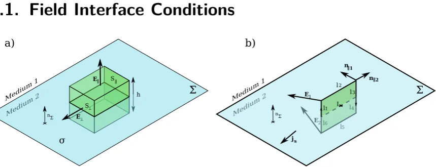
Figure 3.1.: a) The normal field interface conditions are obtained by considering

the flux of the fields through an infinitely small box containing the surface Σ with a surface charge σ. b) The tangential field interface conditions are obtained by

considering the circulation of the fields in a rectangle crossing the surface Σ with a surface current js, and by making the square infinitely small.

3.1.1. Normal Fields

We consider a surface Σ between two media with a surface charge σ. By using the

Ostrogradsky theorem on a box Figure 3.1.a containing the surface, and the value of the divergence of a field, and by making the length h and the surface of the box Sk go to zero, we obtain the surface conditions for the normal part of this field:



  

  

(E1−E2)·nΣ = ε0σ

(D1−D2)·nΣ = σf

Chapter 3 Interface Conditions

with σf the free surface charge and nΣ the normal vector of the surface.

3.1.2. Tangential Fields

In the same way, through using the Stokes theorem on a rectangle crossing the surface Figure 3.1.b , by making all the lengths l1→6 equal and approaching 0 and

by using the expression of the Curl of a field, we obtain the surface conditions for

the tangential part of this field:



  

  

(E1−E2)×nΣ = 0

(H1−H2)vnΣ = jS,free×nΣ (B1−B2)×nΣ = µ0jS,free×nΣ

3.1.3. Poynting Vector

We use the interface conditions that we just obtained to see how the Poynting vector

Π behaves at the interface. With the Xk the component of a vector X parallel to

the surface, andX⊥ the tangential component, we can write:

Π=E×H= (Ek+E⊥)×(Hk+H⊥) =Ek×Hk

| {z }

Π⊥

+EkvH⊥+E⊥×Hk

| {z }

Πk

.

Ekis conserved at the interface andHkis conserved if the free charges at the interface

are zero, which we will always assume to be true in this thesis. So we obtain:

(Π1−Π2)×nΣ= 0

3.2. Fresnel Equations

We consider the interface between two dielectric materials 1 and 2 to be isotropic, or anisotropic but with the principal axis (c1 and c2) limited to being along one of the axes (ex,ey,ez). We suppose an incident fieldEi to be coming from the left and splitting at the interface between a reflected beam Er and a transmitted beam Et. The different fields are given by:

Em(r, t) = Em0exp[ikm.r−iωt]

3.2 Fresnel Equations

n

n

k

k

k

X Z

θ_t θ_i

Figure 3.2.: Incident, reflected and transmitted wave vectors ki, kr and kt at the

interface between two materials of index n1 and n2.

Where m= (i, r, t). We suppose the propagation of the incident beam to be in the

plane (ex,ez), which means that we have ki∈(ex,ez) .

The tangential part of the electric field Ek is conserved at the interface:

Eik+Erk =Etk

We get for all time t and all points r on the surface:

Ei0kexp[iki·r−iωit] +Er0kexp[ikr·r−iωrt] =Et0kexp[ikt·r−iωtt]

This means that the frequencies of each field are the same ωi = ωr = ωt and that

we have equality in the tangential wave vectors kik = krk = ktk, corresponding to

the first law of Snell-Descartes. We suppose that the incident beam is given by:

ki =



 

kix

0

kiz





.

Knowing that each wave vector verifies: ||km|| = nmω_c , with nm the index

experi-enced by the light in the medium m at this particular polarization, we obtain:

kr =



 

kix

0

−kiz





 kt=



   

kix

0

n2ω_c

2

−(kix) 21/2



   

.

If the incident beam is real, we consider θi such that kix = n1sin(θi) and kiz =

n1cos(θi), and if we have the two indices respecting: n_n1₂ sin(θi)≤1. We obtain the

Chapter 3 Interface Conditions

n1sin(θi) =n2sin(θt)

with θt such that ktx=n2sin(θt) andktz =n2cos(θt).

If the crystal on the left is isotropic Figure 3.2, we consider the s-polarization with the electric field along ey and the p-polarization with the electric field in the plane (ex,ez) perpendicular to k. If the crystal is anisotropic with the extraordinary axis c1 along ey, the problem is the same. The ordinary beam polarization Eo is perpendicular to the extraordinary axis c1 and the wave vector k, so it is in the plane (ex,ez) (p-polarization case), and the extraordinary polarization Ee is along ey (s-polarization case) because k is orthogonal to the extraordinary axis

c1(subsection 2.2.3). If the crystal is anisotropic with the extraordinary axis c1 along ex or ez, the ordinary polarization Eo is perpendicular to the extraordinary axis andk, soEo is alongey(s-polarization case), and the extraordinary polarization

Ee is perpendicular to the ordinary polarization, so Ee is in the plane (ex,ez) (but

Ee⊥k is no longer necessarily true).

The same reasoning used on the crystal on the right shows that the s-polarization and p-polarization are good common bases for the problem.

From now on, in calculations, we will omit exp(−iωt) for simplicity.

3.2.1. TE Polarization or S-Polarization

The incident electric field Ei is supposed to be polarized in the ey axis. The three electric fields’ expressions are:



 

 

Ei = E0eyexp[i(kixx+ikizz)]

Er = rsE0eyexp[i(kixx−ikizz)]

Et = tsE0eyexp[i(kixx+iktzz)]

, (3.1)

with rs and ts the reflection and transmission factors.

The continuity of Ek gives a first equation:

E0+rsE0 =tsE0. (3.2)

Maxwell-Faraday equation: ∇ ×E = iωB gives in the x direction: ∂Ey_∂z = −iωBx.

The continuity of B⊥ gives the continuity of ∂Ey_∂z , which gives the second equation:

kizE0−rskizE0 =ktztsE0. (3.3)

3.2 Fresnel Equations

We have two equations with two variables:

(

1 +rs = ts

kiz(1−rs) = ktzts

,

These equations can easily be solved and give:



 

 

r

=

t

=

2kiz

ktz+kiz

.

If kiz and ktz are real, we can rewrite these coefficients:







rs = n_n1cos(θi)−n2cos(θt)

2cos(θt)+n1cos(θi)

ts = _n2cos(θt)+n2n1cos(θi)_1cos(θi)

.

The interesting values to measure are the reflectanceR= |Πr⊥|

|Πi⊥| and transmittance of the systemT = |Πt⊥|

|Πi⊥|, with Πi⊥,Πr⊥ and Πt⊥the normal components of the incident, the reflected, and the transmitted Poynting vectors Π⊥ = Ek ×Hk. By using the

Maxwell-Faraday equation ∇ ×E=−∂B

∂t we can calculate the parallel magnetizing

field Hx =−_ωµkz₀Ey and Hy = 0.



 

 

R = |Erk×Hrk|

|Eik×Hik| =r

2 s

T = |Etk×Htk|

|Eik×Hik| =t

2 sktzkiz

.

They represent the reflection and transmission of the energy through the surface. The conservation of energy implies R+T = 1.

3.2.2. TM Polarization or P-Polarization

We suppose here that the electric fields E are in the plane (ex,ez). For the calcula-tion, we will consider the field H which is only in the direction ey. We will define the same coefficient, but for the Hfield instead:



 

 

Hi = H0eyexp[i(kixx+ikizz)]

Hr = rHH0eyexp[i(kixx−ikizz)]