A Graph Kernel based on Jensen-Shannon Representation

This is a repository copy of A Graph Kernel based on Jensen-Shannon Representation.

White Rose Research Online URL for this paper:

http://eprints.whiterose.ac.uk/88205/

Version: Submitted Version

Proceedings Paper:

Bai, Lu, Zhang, Zhihong and Hancock, Edwin R orcid.org/0000-0003-4496-2028 (2015) A

Graph Kernel based on Jensen-Shannon Representation. In: International Joint

Conference on Artificial Intelligence (IJCAI). .

[email protected] https://eprints.whiterose.ac.uk/ Reuse

Items deposited in White Rose Research Online are protected by copyright, with all rights reserved unless indicated otherwise. They may be downloaded and/or printed for private study, or other acts as permitted by national copyright laws. The publisher or other rights holders may allow further reproduction and re-use of the full text version. This is indicated by the licence information on the White Rose Research Online record for the item.

Takedown

If you consider content in White Rose Research Online to be in breach of UK law, please notify us by

A Graph Kernel Based on the Jensen-Shannon Representation Alignment

∗

Lu Bai

1

,2†

, Zhihong Zhang

3‡

, Chaoyan Wang

4

, Xiao Bai

5

, Edwin R. Hancock

2

1

School of Information, Central University of Finance and Economics, Beijing, China

2

Department of Computer Science, University of York, York, UK

3

Software School, Xiamen University, Xiamen, Fujian, China

4

School of Contemporary Chinese Studies, University of Nottingham, Nottingham, UK

5

School of Computer Science and Engineering, Beihang University, Beijing, China

Abstract

In this paper, we develop a novel graph kernel by aligning the Jensen-Shannon (JS) representations of vertices. We commence by describing how to compute the JS representation of a vertex by mea-suring the JS divergence (JSD) between the

cor-responding h-layer depth-based (DB)

representa-tions developed in [Baiet al., 2014a]). By

align-ing JS representations of vertices, we identify the correspondence between the vertices of two graphs and this allows us to construct a matching-based graph kernel. Unlike existing R-convolution ker-nels [Haussler, 1999] that roughly record the iso-morphism information between any pair of sub-structures under a type of graph decomposition, the

new kernel can be seen as analigned subgraph

kernel that incorporates explicit local

correspon-dences of substructures (i.e., the local information

graphs [Dehmer and Mowshowitz, 2011]) into the process of kernelization through the JS representa-tion alignment. The new kernel thus addresses the drawback of neglecting the relative locations be-tween substructures that arises in the R-convolution kernels. Experiments demonstrate that our kernel can easily outperform state-of-the-art graph kernels in terms of the classification accuracies.

1

Introduction

There have been many successful attempts to classify or

cluster graphs using graph kernels [G¨artner et al., 2003;

Jebaraet al., 2004; Barra and Biasotti, 2013; Harchaoui and

Bach, 2007]. The main advantage of using graph kernels is that they characterize graph features in a high dimensional space and thus better preserve graph structures. A graph ker-nel is usually defined in terms of a similarity measure be-tween graphs. Most of the recently developed graph kernels are instances of the family of R-convolution kernels proposed

∗_{This work is supported by the National Natural Science}

Foun-dation of China (61402389 and 61272398). Edwin R. Hancock is supported by a Royal Society Wolfson Research Merit Award.

†_{Primary Author: [email protected]; [email protected]}

‡_{Corresponding Author: [email protected].}

by Haussler [Haussler, 1999], which provide a generic way of defining graph kernels by comparing all pairs of isomor-phic substructures under decomposition, and a new decom-position will result in a new graph kernel. Generally speak-ing, the R-convolution kernels can be categorized into the following classes, namely graph kernels based on compar-ing all pairs of a) walks (e.g., the random walk kernel [Jebara

et al., 2004]), b) paths (e.g., the shortest path kernel [Borg-wardt and Kriegel, 2005]), c) cycles (e.g., the backtracless kernel from the cycles identified by the Ihara zeta function

[Aziz et al., 2013]), and d) subgraph or subtree structures

(e.g., the subgraph or subtree kernel [Costa and Grave, 2010;

Shervashidzeet al., 2011]).

One drawback arising in the R-convolution kernels is that they neglect the relative locations of substructures. This oc-curs when an R-convolution kernel adds an unit value to the kernel function by roughly identifying a pair of isomorphic substructures. As a result, the R-convolution kernels can-not establish reliable structural correspondences between the substructures. This drawback limits the precise kernel-based similarity measure for graphs.

To overcome the shortcomings of existing R-convolution kernels, we propose a novel matching kernel by aligning JS representations of vertices, which are computed based

on the JSD measure [Bai et al., 2012; Bai and Hancock,

2013] between DB representations [Bai and Hancock, 2014] of graphs. The main advantages of using DB representa-tions and the JSD measure are twofold. First, in the

liter-ature [Crutchfield and Shalizi, 1999; Escolano et al., 2012;

Bai and Hancock, 2014], DB representations of graphs are powerful tools for characterizing graphs in terms of complex-ity measures and reflect rich depth characteristics of graphs.

Second, in the litearturethe [Baiet al., 2012; Bai, 2014], the

JSD measure of graphs can not only reflect the information theoretic (dis)similarities between entropies of graphs but can also be efficiently computed for a pair of large graphs. As a result, the DB representation and the JSD measure provide us an elegant way of defining new effective graph kernels.

To compute the new matching kernel, for each graph

un-der comparison, we commence by computing theh-layer DB

representation of each vertex, that has been previously

in-troduced in [Baiet al., 2014a]. Moreover, we determine a

m-sphere (i.e., a vertex set) for each vertex by selecting the

vertices that have the shortest path lengthm to the vertex.

We compute a newm-layer JS representation for each

ver-tex by measuring the JSD between the h-layer DB

repre-sentations of the vertex and the vertices from its m-sphere.

The m-layer JS representation rooted at a vertex not only

encapsulates a high-dimensional entropy-based depth infor-mation for the vertex, but also reflects the co-relation

be-tween the vertex and itsm-sphere vertices (i.e., the JS

repre-sentation reflects richer characteristics than the original DB

representation). Based on the new JS representations for

two graphs we develop a new vertex matching strategy by

aligning the JS representations. Finally, we compute the

new kernel, namely the JS matching kernel, for graphs by counting the number of matched vertex pairs. We theoreti-cally show the relationship between our kernel and the clas-sical all subgraph kernel and explain the reason for the ef-fectiveness of our kernel. Our JS matching kernel can be

seen as an aligned subgraph kernel that counts the

num-ber of aligned isomorphic subgraph (i.e., the local informa-tion graph [Dehmer and Mowshowitz, 2011]) pairs which are correspond by the corresponding aligned JS representa-tions. Our kernel thus overcomes the mentioned shortcoming of neglecting the structural correspondence information be-tween substructures that arises in R-convolution kernels. Fur-thermore, compared to the DB matching kernel that is

com-puted by aligning theh-layer DB representations [Bai, 2014;

Baiet al., 2014a], our kernel not only reflects richer char-acteristics but also identifies more pairs of isomorphic sub-graphs that encapsulate the structural correspondence infor-mation. We empirically demonstrate the effectiveness of our new kernel on graphs from computer vision datasets.

2

Vertex Matching using JS Representations

In this section, we define a JS representation for a vertex and a vertex matching method by aligning the representations.

2.1

The JSD Measure for Graphs

In this work, we require the JSD measure for graphs. In mu-tual information, the JSD is a dissimilarity measure for prob-ability distributions in terms of the entropy difference

asso-ciated with the distributions [Martins et al., 2009]. In [Bai

and Hancock, 2013; Bai et al., 2012], Bai et al. have

ex-tended the JSD measure to graphs for the purpose of com-puting the JSD based information theoretic graph kernels. In their work, the JSD between a pair of graphs is computed by measuring the entropy difference between the entropies of the graphs and those of a composite graph (e.g., the disjoint

union graph [Baiet al., 2012]) formed by the graphs. In this

subsection, we generalize their work in [Baiet al., 2012] and

give the concept of measuring the JSD for a set of graphs. Let G_{= {Gn|n= 1,2, . . . , N} denote a set ofN graphs, and}

Gn(Vn, En)is a sample graph inGwith vertex setVn and

edge setEn. The JSD measureDfor the set of graphsGis

D(G_{) =HS(GDU)−} 1

N

N

X

n=1

HS(Gn), (1)

where HS(Gn) is the Shannon entropy for Gn associated

with steady state random walks [Bai and Hancock, 2013] and

is defined as

HS(Gn) =−

X

v∈Vn

PGn(v) logPGn(v), (2)

wherePGn(v) =Dn(v, v)/

P

u∈V Dn(u, u)is the

probabil-ity of the steady state random walk visiting the vertexv∈Vn,

and D is the diagonal degree matrix of Gn. Moreover, in

Eq.(1) GDU is the disjoint union graph formed by all the

graphs inG_{, andHS(GDU)is the Shannon entropy of the}

union graph. Based on the definition in [K¨oner, 1971], the entropy of the disjoint union graph is defined as

HS(GDU) =

PN

n=1|Vn|HS(Gn)

PN

n=1|Vn|

, (3)

where|Vn|is the number of vertices ofGn. Eq.(1) and Eq.(3)

indicate that the JSD measure for a pair of graphs can be di-rectly computed from their vertex numbers and entropy val-ues. Thus, the JSD measure can be efficiently computed.

2.2

The JS Representation through the JSD

In this subsection, we compute am-layer JS representation

around a vertex for a graph. To commence, we first review

the concept of theh-layer DB representation around a vertex.

This has been previously introduced by Bai et al. [Baiet al.,

2014a], by generalizing the DB complexity trace around the centroid vertex [Bai and Hancock, 2014]. For an undirected

graphG(V, E)and a vertexv ∈ V, let a vertex setNK

v be

defined as NK

v = {u ∈ V | SG(v, u) ≤ K}, where SG

is the shortest path matrix ofGandSG(v, u)is the shortest

path length betweenvandu. ForG, theK-layer expansion

subgraphGK

v (VvK;EvK)aroundvis

VK

v ={u∈NvK}; EK

v ={u, v∈NvK, (u, v)∈E}.

(4)

For the graphG, theh-layer DB representation aroundvis

DBh_G(v) = [HS(Gv1),· · ·, HS(GvK),· · ·, HS(Gvh)]T, (5)

where (K ≤ h), GK

v is the K-layer expansion subgraph

aroundv, andHS(GvK)is the Shannon entropy ofGvKand is

defined in Eq.(2). Note that, ifLmaxis the greatest length

of the shortest paths from v to the remaining vertices and

K≥Lmax, theK-layer expansion subgraph isGitself.

Clearly, theh-layer DB representationDBhG(v)reflects an

entropy-based information content flow through the family of

K-layer expansion subgraphs rooted at v, and thus can be

seen as a vectorial representation ofv.

Them-layer JS representation:For the graphG(V, E)and

the vertexv ∈ V, we define them-sphere (i.e., a vertex set)

aroundv asNˆm

v = {u ∈ V | SG(v, u) = m} (note that,

ˆ

Nm

v is different fromNvK, even ifm = K), based on the

definition in [Dehmer and Mowshowitz, 2011]. The JSD for

theh-layer DB representations ofvand the vertices inNˆK

v is

D_G(m;h)(v) = [D(G1_ˆ

Nm

v ), . . . ,D(

GK_ˆ

Nm

v ), . . . ,D(

Gh_ˆ

Nm v )]

T_,

whereGK_ˆ

Nm v

is a graph set and consists of theK-layer

expan-sion subgraphs aroundvand the vertices inNˆm

v . Them-layer

JS representation around the vertexvis

J_G(m;h)(v) =D_G(m;h)(v) +DBhG(v). (7)

Note that, the dimension of Jm

G(v) is equal to that of

DBhG(v), i.e., JGm(v) is a h dimensional vector. This can

be observed from Eq.(5), Eq.(6) and Eq.(7). 2

Discussions: Compared to the h-layer DB representation

DBhG(v), the m-layer JS representationJ

(m;h)

G (v)not only

reflects the information content (i.e., the entropy) flow rooted

at the vertexvrelying onDBhG(v), but also encapsulates the

entropy-based dissimilarity information (or the relationship)

between the h-layer DB representation ofv and that of the

vertices inNˆm

v in terms of the JSD measureD

(m;h)

G (v). In

other word, for each vertex them-layer JS representation

re-flects richer characteristics than its originalh-layer DB

rep-resentation. This can be observed from Eq.(7). Moreover, based on the definition proposed by Dehmer and Mowshowitz in [Dehmer and Mowshowitz, 2011], the shortest paths

de-parting fromvto the vertices inNˆm

v can be used to form a

lo-cal information graphLG(v, m)rooted atv. SinceLG(v, m)

is encompassed or determined by them-sphereNˆm

v around

v, the vertexv and itsm-sphere play a crucial role of

gen-eratingLG(v, m). As a result, them-layer JS representation

J_G(m;h)(v)can also be seen as a vectorial signature for the

lo-cal information graphLG(v, m). Details of local information

graphs can be found in [Dehmer and Mowshowitz, 2011].

2.3

Vertex Matching from the JS Represenations

We propose a new vertex matching method, namely the JS matching method, for a pair of graphs by aligning their JS representations of vertices. Our matching method is similar to that previously introduced by Scott et al. in [Scott and Longuett-Higgins, 1991] for point set matching, that com-putes an affinity matrix in terms of the distances between

points. For a pair of graphs Gp(Vp, Ep) and Gq(Vq, Eq),

we use the m-layer JS representations J_G(m_p;h)(vi) and

J_G(m_q;h)(uj), that are computed from the corresponding h

-layer DB representations, as the point coordinates for the

ver-tices vi ∈ Vp anduj ∈ Vq, respectively. ForGp andGq,

we compute the Euclidean distance betweenJ_G(m_p;h)(vi)and

J_G(m_q;h)(uj)as the elementR(m;h)(i, j)of their affinity matrix

R(m;h)_{, andR}(m;h)_{(i, j)is defined as}

R(m;h)_{(i, j) =kJ}(m;h)

Gp (vi)−J (m;h)

Gq (uj)k2. (8)

whereR(m;h)_{is a|V}

p| × |Vq|matrix, and the parametersm

andhindicate that the affinity matrix is computed from the

m-layer JS representation over theh-layer DB representation.

R(m;h)_{(i, j)represents the distance or dissimilarity between}

the vertexviinGpand the vertexujinGq. Furthermore, for

the affinity matrixR(m;h)_{, the rows index the vertices ofG}

p,

and the columns index the vertices ofGq.

If R(m;h)_{(i, j) is the smallest element simultaneously in}

rowiand in column j, moreover|Nˆm

vi| = | ˆ

Nm

uj| 6= 0(i.e.,

the vertex number of the m-sphere aroundvi ∈ Vp is equal

to that arounduj ∈Vq, and these vertex numbers also cannot

be0), there should be a one-to-one correspondence between

the vertexvi ofGp and the vertexuj ofGq, i.e., vi anduj

are matched. We record the state of correspondence using the

correspondence matrixC(m;h)_{∈ {0,1}}|Vp|×|Vq|_{that satisfies}

C(m;h)_{(i, j) =}



  

  

1 ifR(i, j) is the smallest element,

both in rowiand in column j,

and|Nˆm vi|=|Nˆ

m uj| 6= 0; 0 otherwise.

(9)

Eq.(9) indicates that ifC(m;h)_{(i, j) = 1, the verticesv}

iand

vjare matched. Moreover, the condition|Nˆvmi|=|Nˆ

m uj| 6= 0

for Eq.(9) guarantees that both of the m-spheres|Nˆm

vi|and

|Nˆm

uj|are not empty vertex sets.

Note that, similar to the DB matching previously

intro-duced by Bai et al. [Baiet al., 2014a], for a pair of graphs

a vertex from a graph may have more than one matched ver-tices from the other graph. In our work, we propose to assign a vertex at most one matched vertex. One way to achieve this

is to update the matrixC(m;h)_{by adopting the Hungarian}

al-gorithm [Munkres, 1957] that can solve the assignment

prob-lem, following the strategy proposed in [Bai et al., 2014a].

Here, the matrixC(m;h) _{∈ {0,1}}|Vp|×|Vq|_{can be seen as the}

incidence matrix of a bipartite graphGpq(Vp, Vq, Epq), where

Vp andVq are the two sets of partition parts andEpq is the

edge set. By performing the Hungarian algorithm on the

ma-trixC(m;h)_{, we can assign each vertex from the partition part}

VporVq at most one matched vertex from the other partition

part Vq orVp. Unfortunately, the Hungarian algorithm

usu-ally requires extra expansive computation and thus may lead to computational inefficiency for the JS matching. To address the inefficiency, an alternative way or strategy is to randomly assign each vertex an unique matched vertex through the

cor-respondence matrix C(m;h)_{. In other words, for the}

corre-spondence matrixC(m;h)_{, from the first row and the first}

col-umn, we will set each evaluating element of C(m;h) _{as0 if}

there has been an existing element that is1either in the same

row or the same column. Based on our evaluations, this strat-egy will not influence the effectiveness of our resulting kernel in Section 3, and the kernel using the strategy will be more ef-ficient than that using the Hungarian algorithm.

3

A Graph Kernel from the JS Matching

In this section, we propose a new graph kernel from the JS vertex matching by aligning the JS representations of vertices.

3.1

The Jensen-Shannon Matching Kernel

Definition (The Jensen-Shannon matching kernel):

Con-sider a pair of graphs asGp(Vp, Ep)andGq(Vq, Eq). Based

on the definition of JS matching introduced in Section 2.3, we

commence by computing the correspondence matrixC(m;h)_.

representations, for the graphs is

k_{J SM}(M;h)(Gp, Gq) = M

X

m=1

|Vp|

X

i=1

|Vq|

X

j=1

C(m;h)_{(i, j),}

(10)

whereM is the greatest value of the parameter m(i.e., m

varies from1toM). Eq.(10) indicates thatk_{J SM}(M;h)(Gp, Gq)

counts the number of matched vertex pairs betweenGp and

Gqover theM correspondence matricesC(m;h). 2

Lemma.The matching kernelk_{J SM}(M;h)is positive definite (pd).

Proof. Intuitively, the proposed JS matching kernel is pd

because it counts pairs of matched vertices (i.e., the

small-est subgraphs) over theM correspondence matricesC(m;h)_.

More formally, let the base counting kernel km _{be a}

func-tion counting pairs of matched vertices between the graphs

GpandGq from the correspondence matrixC(m;h), and

km_(G

p, Gq) =

X

vi∈Vp

X

uj∈Vq

δ(vi, uj), (11)

where

δ(vi, uj) =

1 ifC(i, j) = 1;

0 otherwise. (12)

whereδis the Dirac kernel, that is, it is1 if the arguments

are equal and0otherwise (i.e., it is1if a pair of vertices are

matched and0otherwise). From the base counting kernelkm_,

the JS matching kernelk(_{J SM}M;h)can be re-written as

k_{J SM}(M;h)(Gp, Gq) = M

X

m=1

km_(G

p, Gq). (13)

Eq.(11) indicates that the base counting kernelkm_{is the sum}

of pdDirac kernels and is thuspd. As a result, the kernel

k(_{J SM}M;h)summing the positive definite kernelkm_ispd.

3.2

Relation to the All Subgraph Kernel

The JS matching kernel can be re-defined in another manner that elucidates its advantage and effectiveness, compared to the all subgraph (AS) kernel. To commence, we review the definition of the AS kernel introduced in [Borgwardts, 2007].

LetGp(Vp, Ep)andGq(Vq, Eq)be a pair of graphs for the

kernel computation. The AS kernel is defined as

kAS(Gp, Gq) =

X

Sp⊑Gp

X

Sq⊑Gq

kI(Sp, Sq), (14)

where

kI(Sp, Sq) =

1 ifSp≃Sq,

0 otherwise. (15)

Below, we re-define the JS matching kernel in a manner that is similar to the AS kernel. Based on the definition in

Section 2.2, them-layer JS representations around a vertex

v ∈ Vp ofGp(Vp, Ep)and a vertexu ∈ Vq of Gq(Vq, Eq)

are J_G(m;h)

p (v) = D

m

Gp(v) +DB

h

Gp(v) and J (m;h)

Gq (u) =

Dm

Gq(u) +DB

h

Gq(u), respectively. According to the

discus-sions in Section 2.2, eachm-layer JS representation around

a vertex can be seen as a vectorial signature of a local

infor-mation graph, which is determined by the vertex and them

-sphere around the vertex. Based on the JS matching defined

in Section 2.3, if the verticesv anduare matched, the two

m-layer JS representations around the two vertices are close

together in a corresponding principle space. Thus, the

corre-sponding local information graphsLGp(v, m)aroundv∈Vp

andLGq(u, m)aroundu ∈ Vq can be seen as approximate

isomorphism, i.e.,LGp(v, m)≃LGq(u, m). As a result, the

JS matching kernelk_{J SM}(M;h)can be re-written as

k(_{J SM}M;h)(Gp, Gq) =

X

Sp⊑Gp

X

Sq⊑Gq

kI(Sp, Sq), (16)

where

kI(Sp, Sq) =



 

 

1 ifSp=LGp(v, m) andLGq(u, m),

vanduare matched,

and|Nˆm

v |=|Nˆum| 6= 0;

0 otherwise.

(17)

Here, the condition|Nˆm

vi|=|Nˆ

m

uj| 6= 0of Eq.(17) guarantees

that them-spheresNˆm

v andNˆumexist, i.e., the local

informa-tion graphs LGp(v, m)and LGq(u, m) that are determined

by them-spheres exist. This is because an emptym-sphere

cannot form a local information, more details can be found in [Dehmer and Mowshowitz, 2011].

Discussions: Through Eq.(14) and Eq.(17), we observe that

both the kernelskAS andk(_{J SM}M;h)need to identify any pair of

isomorphic subgraphs. ForkASandkJ SM(M;h), each pair of

iso-morphic subgraphs pair will add an unit value to the kernel function, i.e., both the AS kernel and our JS matching kernel count the number of isomorphic subgraph pairs. However, we also observe that there are two significant differences be-tween the AS kernel and the JS matching kernel. First, for the JS matching kernel, only the subgraphs (i.e., the local in-formation graphs) around a pair of matched vertices that are

determined by the vertices and them-spheres around the

ver-tices are evaluated with respect to be isomorphic. By con-trast, for the AS kernel, any pair of subgraphs are evaluated for identifying the isomorphism. As a result, the JS matching kernel overcomes the NP-hard problem of measuring all pos-sible pairs of subgraphs that arises in the AS kernel. Second, for the JS matching kernel, any pair of isomorphic local in-formation graphs are identified by a pair of matched vertices

and them-spheres around the vertices. Thus, there is a

loca-tional correspondence between the isomorphic local informa-tion graphs (i.e., the corresponding subgraphs) with respect to the global graphs. By contrast, a pair of subgraphs hav-ing no location correspondence may also be seen as isomor-phism by the AS kernel. The above observations indicate that

our JS matching kernel is essentially analigned subgraph

3.3

Discussions and Related Work

Clearly, the JS matching kernel is related to the DB represen-tation defined in [Bai and Hancock, 2014]. However, there are two significant differences. First, the DB representation is computed by measuring the entropies of subgraphs rooted at the centroid vertex. The centroid vertex is identified by evaluating the minimum shortest path length variance to the remaining vertices. By contrast, in our work, we first compute

theh-layer DB representation rooted at each vertex, and then

compute the resultingm-layer JS representation. For a

ver-tex, itsm-layer JS representation is computed by summing its

DB representation and the JSD measure between its DB

rep-resentation and that of the vertices from itsm-sphere.

Sec-ond, in [Bai and Hancock, 2014] the DB representation from the centroid vertex is a vectorial signature of a graph, i.e., it can be seen as an embedding vector for the graph. Embed-ding a graph into a vector tends to approximate the structural correlations in a low dimensional space, and thus leads to in-formation loss. By contrast, the JS matching kernel aligning

them-layer JS representation represents graphs in a high

di-mensional space and thus better preserves graph structures. On the other hand, the DB matching kernel developed in [Baiet al., 2014a] is also related to the DB representation in [Bai and Hancock, 2014]. Moreover, similar to our JS match-ing kernel, the DB matchmatch-ing kernel can also better preserve graph structures by kernelizing the DB representation. How-ever, unlike the JS matching kernel, this kernel is computed

by aligning theh-layer DB representation rather than

align-ing them-layer JS representation. According to the statement

in Section 2.2, them-layer JS representation for a vertex

re-flects richer characteristics than its originalh-layer DB

rep-resentation. As a result, the JS matching kernel can capture more information for graphs than the DB matching kernel. Moreover, Bai [Bai, 2014] also demonstrates the relationship between the DB matching kernel and the AS kernel. The DB matching kernel can also be re-defined as a manner that is similar to the AS kernel, i.e., the DB matching kernel can be seen as a subgraph kernel that counts the number of

ap-proximately isomorphich-layer (i.e.,K=h) expansion

sub-graph pairs. Each pair of isomorphich-layer expansion

sub-graphs are identified by a pair of matched vertices from the DB matching. Thus, similar to our JS matching kernel, the DB matching kernel can also reflect the locational correspon-dence information between each pair of identified isomorphic subgraphs. Unfortunately, the identified isomorphic subgraph pair number of the DB matching kernel is less than that of the

JS matching kernel. For a pair of graphs each havingx

ver-tices, the DB matching kernel can only identify xpairs of

isomorphic subgraphs at most. By contrast, the JS

match-ing kernel can identifyM xpairs of isomorphic subgraphs at

most. This again demonstrates that our JS matching kernel captures more information than the DB matching kernel.

Finally, like the JS graph kernel [Bai and Hancock, 2013], our kernel is also related to the JSD. However, the JS graph kernel only reflects the global similarity of graphs in terms of the JSD measure between a pair of global graphs, and lacks the interior topological information of graphs. By contrast, our JS matching kernel can reflect rich vertex correspondence information from the JS representations computed by

measur-ing the JSD between correspondmeasur-ing DB representations.

4

Experimental Results

We demonstrate the performance of our new kernel on three standard graph datasets from computer vision databases. The reason of using computer vision datasets is that many com-puter vision applications usually require the correspondence information between pairwise feature points that are ab-stracted from images or 3D shapes, for the objective of simi-larity measure. For an instance, one has two graphs abstracted from two digital images both containing the same object, based on different viewpoints. Here, each vertex represents a feature point. Identifying the correspondence information between pairwise vertices or substructures from the identical region is our concern, and can provide us an elegant way of reflecting precise similarity between the images or shapes. As a result, the new matching kernel can easily indicate its main advantage of identifying the correspondence information, on computer vision datasets. The advantage is unavailable for most existing graph kernels from R-convolution.

BAR31, BSPHERE31 and GEOD31: The SHREC 3D

Shape database consists of15classes and 20 individuals per

class, that is 300 shapes [Biasotti et al., 2003]. This is a

usual benchmark in 3D shape recognition. From the SHREC 3D Shape database, we establish three graph datasets named BAR31, BSPHERE31 and GEOD31 datasets through three mapping functions. These functions are a) ERG barycen-ter: distance from the center of mass/barycenter, b) ERG bsphere: distance from the center of the sphere that circum-scribes the object, and c) ERG integral geodesic: the average of the geodesic distances to the all other points. The num-ber of maximum, minimum and average vertices for the three datasets are a) 220, 41 and 95.42 (for BAR31), b) 227, 43 and 99.83 (for BSPHERE31), and c) 380, 29 and 57.42 (for GEOD31), respectively.

4.1

Experiments on Graph Datasets

Experimental Setup: First, we evaluate the performance of our JS matching kernel (JSMK) on graph classification problems. We also compare our kernel with several alter-native state-of-the-art graph kernels. These graph kernels include 1) the DB matching kernel (DBMK) [Bai, 2014; Bai et al., 2014a], 2) the Weisfeiler-Lehman subtree

ker-nel (WLSK) [Shervashidzeet al., 2011], 3) the shortest path

graph kernel (SPGK) [Borgwardt and Kriegel, 2005], 4) the

graphlet count graph kernel [Shervashidzeet al., 2009] with

graphlet of size4(GCGK) [Shervashidzeet al., 2009], 5) the

un-aligned quantum Jensen-Shannon kernel (UQJS) [Bai et

al., 2015], 6) the Jensen-Shannon graph kernel (JSGK) [Bai

and Hancock, 2013], and 7) the Jensen-Tsallis q-difference

kernel (JTQK) [Baiet al., 2014b] associated withq= 2. For

our JS matching kernel k(_{J SM}M;h), we set the has 10and the

greatest value ofmas40(i.e.,M = 40). For the WLSK

ker-nel and the JTQK kerker-nel, we set the highest dimension (i.e., the highest height of subtrees) of the Weisfeiler-Lehman iso-morphism (for the WLSK kernel) and the tree-index method

(for the JTQK kernel) as10. For the DBMK kernel, we set

each kernel, we compute the kernel matrix on each graph

dataset. We perform 10-fold cross-validation using the

C-Support Vector Machine (C-SVM) Classification to compute the classification accuracies, using LIBSVM [Chang and Lin, 2011]. We use nine samples for training and one for testing. All the C-SVMs were performed along with their parame-ters optimized on each dataset. We repeat the experiment 10 times. We report the average classification accuracies and standard errors for each kernel in Table.1.

Experimental Results: In terms of the classification accu-racies, our JSMK kernel can easily outperform all the alter-native graph kernels on any dataset. The classification accu-racies of our JSMK kernel are obviously higher than those of all the alternative kernels. The reasons for the effective-ness are threefold. First, compared to the WLSK, SPGK, GCGK and JTQK kernels that require decomposing graphs into substructures, our JSMK kernel can establish the sub-structure location correspondence which is not considered in these kernels. Second, compared to the JSGK and QJSK ker-nels that rely on the similarity measure between global graphs in terms of the classical or quantum JSD, our JSMK kernel can identify the correspondence information between both the vertices and the substructures, and can thus reflect richer in-terior topological characteristics of graphs. By contrast, the JSGK and QJSK kernels can only reflect the global similarity information between graphs. Third, compared to the DBMK kernel that can also reflect the correspondence information between substructures, our JSMK kernel can identify more pairs of aligned isomorphic substructures. Moreover, as we

have stated in Section 3.3, them-layer JS representation can

reflect richer characteristics than theh-layer DB

representa-tion. As a result, the JSMK kernel using the JS representation can capture more information for graphs than the DBMK ker-nel using the DB representation.

1 2 3 4 5 6 7 8 9 10

0.2 0.3 0.4 0.5 0.6 0.7 0.8 0.9

Classification Accuracies (%)

Layer h of DB Representations BAR31 BSPHERE31 GEOD31

5 10 15 20 25 30 35 40 45 50 0.4

0.45 0.5 0.55 0.6 0.65 0.7 0.75 0.8

Classification Accuracies (%)

[image:7.612.334.531.54.235.2]

Greatest Layer M of JS Representations BAR31 BSPHERE31 GEOD31

Figure 1: The Accuracy with Different Parameters h and M.

Comparisons with Increasing hand M: We explore the performance of our JSMK kernel on graph datasets with

in-creasingh (i.e., h = 1,2, . . . ,10when M = 40) and M

(i.e.,M = 5,10,15. . . ,50whenh= 10). We report the

re-sults in Fig.1. In each subfigure, the x-axis gives the varying

ofhorM, and the y-axis gives the classification accuracies

of our JSMK kernel. The lines of different colours represent the results on different datasets. The classification accuracies

tend to become greater with increasinghorM. The reasons

are twofold. First, for the parameterh, the greater theh, the

higher dimensional DB complexity information of our kernel

can be captured. Second, for the parameterM, the greater

theM, the more pairs of aligned isomorphic local

informa-tion graphs can be identified by our kernel.

0 500 1000 1500 2000 0

1 2 3 4 5 6 7 8

Graph size x

Runtime in seconds

(a) For Parameter x

1 2 3 4 5 6 7 8 9 10 0.186

0.188 0.19 0.192 0.194 0.196 0.198

The layer h

Runtime in seconds

(b) For Parameter h

1 2 3 4 5 6 7 8 9 10 0.192

0.194 0.196 0.198 0.2 0.202 0.204 0.206

The greatest layer M

Runtime in seconds

(c) For Parameter M

0 100 200 300 400 500 0

500 1000 1500 2000 2500

The datasize N

Runtime in seconds

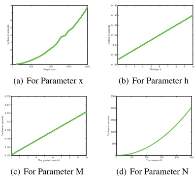
[image:7.612.63.285.443.520.2]

(d) For Parameter N

Figure 2: Runtime Evaluations.

4.2

Computational Evaluations

We explore the computational efficiency (i.e, the CPU run-time) of our JSMK kernel on randomly generated graphs

with respect four parameters: the graph sizen, the layerh

of the DB representations of graphs, the greatest value of

the JS representation layer M, and the graph dataset size

N. We varyx={100,200, . . . ,2000},h={1,2, . . . ,10},

M ={1,2, . . . ,10}, andN ={5,10, . . . ,500}, separately.

a) For the parameterx, we generate20pairs of graphs with

in-creasing number of vertices. We report the runtime for

com-puting the kernel values between pairwise graphs (h = 10

andM = 10). b) For the parameterh, we generate a pair

of graphs each of which has200vertices. We report the

run-time for computing the kernel values of the pair of graphs as a

function ofh(M = 10). c) For the parameterM, we use the

pair of graphs from stepb. We report the runtime for

com-puting the kernel values of the pair of graphs as a function

ofM (h = 10). d) For the parameterN, we generate 500

graph datasets with an increasing number of test graphs. In

each dataset, one graph has200vertices. We report the

run-time for computing the kernel matrices for each graph dataset (h = 10and M = 10). Note that, sinceM = 10, the runtime is for computing the10kernel matrices for each dataset.The CPU runtime is reported in Fig.2, as operated in Matlab R2011b on a 2.5GHz Intel 2-Core processor (i.e., i5-3210m). Fig.2 indicates that the runtime scales cubicly with

n, linearly withhandM, and quadratically withN. These

verify that our kernel can be computed in a polynomial time.

5

Conclusions

Table 1: Classification Accuracy (In%±Standard Error) Using C-SVM and Runtime.

Datasets JSMK DBMK WLSK SPGK GCGK UQJS JSGK JTQK BAR31 75.93±.51 69.40±.56 58.53±.53 55.73±.44 23.40±.60 30.80±.61 24.10±.86 60.56±.35

BSPHERE31 64.46±.66 56.43±.69 42.10±.68 48.20±.76 18.80±.50 24.80±.61 21.76±.53 46.93±.61

GEOD31 50.46±.45 42.83±.50 38.20±.68 38.40±.65 22.36±.55 23.73±.66 18.93±.50 40.10±.46

References

[Azizet al., 2013] Furqan Aziz, Richard C. Wilson, and

Ed-win R. Hancock. Backtrackless walks on a graph. IEEE

Trans. Neural Netw. Learning Syst., 24(6):977–989, 2013.

[Bai and Hancock, 2013] Lu Bai and Edwin R. Hancock.

Graph kernels from the jensen-shannon divergence.

Jour-nal of Mathematical Imaging and Vision, 47(1-2):60–69, 2013.

[Bai and Hancock, 2014] Lu Bai and Edwin R. Hancock.

Depth-based complexity traces of graphs. Pattern

Recog-nition, 47(3):1172–1186, 2014.

[Baiet al., 2012] Lu Bai, Edwin R. Hancock, and Peng Ren. Jensen-shannon graph kernel using information

function-als. InProceedings of ICPR, pages 2877–2880, 2012.

[Baiet al., 2014a] Lu Bai, Peng Ren, Xiao Bai, and Ed-win R. Hancock. A graph kernel from the depth-based

representation. In Proceedings of S+SSPR, pages 1–11,

2014.

[Baiet al., 2014b] Lu Bai, Luca Rossi, Horst Bunke, and Edwin R. Hancock. Attributed graph kernels using the

jensen-tsallis q-differences. In Proceedings of

ECML-PKDD, pages I:99–114, 2014.

[Baiet al., 2015] Lu Bai, Luca Rossi, Andrea Torsello, and

Edwin R. Hancock. A quantum jensen-shannon graph

kernel for unattributed graphs. Pattern Recognition,

48(2):344–355, 2015.

[Bai, 2014] Lu Bai. Information Theoretic Graph Kernels.

University of York, UK, 2014.

[Barra and Biasotti, 2013] Vincent Barra and Silvia Biasotti. 3d shape retrieval using kernels on extended reeb graphs.

Pattern Recognition, 46(11):2985–2999, 2013.

[Biasottiet al., 2003] S. Biasotti, S. Marini, M. Mortara,

G. Patan`e, M. Spagnuolo, and B. Falcidieno. 3d shape

matching through topological structures. InProceedings

of DGCI, pages 194–203, 2003.

[Borgwardt and Kriegel, 2005] Karsten M. Borgwardt and Hans-Peter Kriegel. Shortest-path kernels on graphs. In

Proceedings of ICDM, pages 74–81, 2005.

[Borgwardts, 2007] K.M. Borgwardts. Graph Kernels.

Munchen, 2007.

[Chang and Lin, 2011] C.-C Chang and C.-J. Lin. Libsvm:

A library for support vector machines. Software available

at http://www.csie.ntu.edu.tw/ cjlin/libsvm, 2011.

[Costa and Grave, 2010] Fabrizio Costa and Kurt De Grave. Fast neighborhood subgraph pairwise distance kernel. In

Proceedings of ICML, pages 255–262, 2010.

[Crutchfield and Shalizi, 1999] J.P. Crutchfield and C.R. Shalizi. Thermodynamic depth of causal states: Objective

complexity via minimal representations. Physical Review

E, 59:275283, 1999.

[Dehmer and Mowshowitz, 2011] Matthias Dehmer and

Abbe Mowshowitz. A history of graph entropy measures.

Inf. Sci., 181(1):57–78, 2011.

[Escolanoet al., 2012] F. Escolano, E.R. Hancock, and M.A.

Lozano. Heat diffusion: Thermodynamic depth

complex-ity of networks.Physical Review E, 85:036206, 2012.

[G¨artneret al., 2003] T. G¨artner, P.A. Flach, and S. Wrobel.

On graph kernels: hardness results and efficient

alterna-tives. InProceedings of COLT, pages 129–143, 2003.

[Harchaoui and Bach, 2007] Z. Harchaoui and F. Bach.

Im-age classification with segmentation graph kernels. In

Pro-ceedings of CVPR, 2007.

[Haussler, 1999] D. Haussler. Convolution kernels on

dis-crete structures. Technical Report UCS-CRL-99-10, UC

Santa Cruz, 1999.

[Jebaraet al., 2004] T. Jebara, R.I. Kondor, and A. Howard.

Probability product kernels.Journal of Machine Learning

Research, 5:819–844, 2004.

[K¨oner, 1971] J. K¨oner. Coding of an information source having ambiguous alphabet and the entropy of graphs. In

Proceedings of the 6th Prague Conference on Information Theory, Statistical Decision Function, Random Processes, pages 411–425, 1971.

[Martinset al., 2009] Andr´e F. T. Martins, Noah A. Smith,

Eric P. Xing, Pedro M. Q. Aguiar, and M´ario A. T. Figueiredo. Nonextensive information theoretic kernels

on measures. Journal of Machine Learning Research,

10:935–975, 2009.

[Munkres, 1957] J. Munkres. Algorithms for the assignment

and transportation problems. Journal of the Society for

Industrial and Applied Mathematics, 5(1), 1957.

[Scott and Longuett-Higgins, 1991] G.L. Scott and H.C. Longuett-Higgins. An algorithm fro associating the

fea-tures of two images. InProceedings of the Royal Society

of Londan B, pages 244:313–320, 1991.

[Shervashidzeet al., 2009] N. Shervashidze, S.V.N.

Vish-wanathan, T. Petri, K. Mehlhorn, and K.M. Borgwardt.

Ef-ficient graphlet kernels for large graph comparison.

Jour-nal of Machine Learning Research, 5:488–495, 2009.

[Shervashidzeet al., 2011] Nino Shervashidze, Pascal

Schweitzer, Erik Jan van Leeuwen, Kurt Mehlhorn, and Karsten M. Borgwardt. Weisfeiler-lehman graph kernels.