Transportation Research Procedia 8 ( 2015 ) 50 – 61
2352-1465 © 2015 The Authors. Published by Elsevier B.V. This is an open access article under the CC BY-NC-ND license (http://creativecommons.org/licenses/by-nc-nd/4.0/).
Selection and peer-review under responsibility of Association for European Transport doi: 10.1016/j.trpro.2015.06.041
ScienceDirect
European Transport Conference 2014
–
from Sept-29 to Oct-1, 2014
Re-estimating UK appraisal values for non-work travel time savings
using random coefficient logit model
Jeff Tjiong*
CH2M Hill, Elms House, 43 Brook Green, London W6 7EF, United Kingdom
Abstract
The official appraisal values of travel time savings (VTTS) for non-work trips in UK were estimated by basic discrete choice model on stated choice data collected over 20 years ago. This choice model developed by Bates and Whalen (2001) was specified to address some long-standing issues in the field of VTTS valuation including the sign and size of VTTS while allowing continuous interactions between VTTS and journey covariates. With respect to the size issue, it was found that a “tapering” function, whereby
time changes are increasingly discounted, could best explain the lower unit utility observed for small time savings (STS). While this set of non-work VTTS is still being used for transport appraisal in UK, the field of discrete choice modelling has evolved significantly brought by a leap of computing power and improved simulation techniques. Notably, advanced model such as mixed multinomial logit (MMNL) has been widely used to facilitate more realistic travel behavioural modelling by explaining random taste heterogeneity across respondents, which cannot be achieved in a deterministic manner. Also, techniques in specifying such model for VTTS valuation are well established by researchers nowadays. The key objective of this research was then to apply the MMNL model and re-estimate the current UK VTTS within a random coefficient logit framework. Alongside the theoretical discussions, this paper presents a synthesis of empirical evidence to support an updated appraisal value for non-work travel time savings in UK. Some key findings from this paper include a much higher mean value for the VTTS and the significantly reduced
“perception effect” for the STS. In particular, this research found that MMNL model substantially reduces the “tapering” parameter of the discounting function for STS such that the “perception effect” of the VTTS becomes minimal. This finding suggests that travel benefits due to STS should be included for transport appraisal and it challenges some appraisal frameworks for countries like Germany where VTTS are discounted or even completely ignored for STS.
© 2015 The Authors. Published by Elsevier B. V.
Selection and peer-review under responsibility of Association for European Transport.
Keywords: value of travel time savings, small time savings, random taste heterogeneity, mixtures of distributions
* Corresponding author
E-mail address: [email protected]
© 2015 The Authors. Published by Elsevier B.V. This is an open access article under the CC BY-NC-ND license (http://creativecommons.org/licenses/by-nc-nd/4.0/).
1.Introduction
For many years, high computing costs have created significant obstacles to estimate discrete choice models with flexible specifications such as multinomial probit and mixed multinomial logit (MMNL) models. Amongst these two advanced models, MMNL model is gaining more attention in particular and has become the current state-of-the-art approach (Hess, 2005; Hess et al., 2005), largely facilitated by advances in computing power and simulation techniques in the past decade. Its advantage also lies in the capability to replicate correlation structure of any type of GEV model (McFadden and Train, 2000).
In the field of VTTS valuation, MMNL has already been applied to capture random taste heterogeneity (i.e., variation of VTTS) across respondents. These MMNL models typically assume a mixing distribution to represent the VTTS distribution as a ratio between marginal utilities of travel time and cost in preference space (Algers et al., 1998; Hess et al., 2005; Hess et al., 2008). This research was motivated by these preceding applications and it aims to compare VTTS estimates produced by the basic and advanced choice models.
Two non-work trip purposes, namely commuting trips and other trips, were modelled in the last UK VTTS study by AHCG (1999) and Mackie et al. (2003). For this research, only commuting trips were modelled to narrow the focus such that different MMNL modelling techniques can be exploited to investigate the differences in VTTS due to advanced choice modelling. It should be noted that this research primarily focuses on the comparison of choice modelling methods and is independent of the official VTTS updates being undertaken by the UK Department for Transport at the time of writing.
The remainder of this paper is organised as follows. Section 2 first presents an overview of the mixed logit model concepts. Section 3 summarizes the MNL model specification and findings from the 2001 UK VTTS study. Section 4 provides a summary of MMNL model results and discusses issues involved throughout the modelling process. Section 5 concludes.
2.Theoretical Underpinnings
2.1.MMNL model
The main motivation of the probability mixture model is to mix up different standard and restrictive functions to generate more flexible functions (Walker and Ben-Akiva, 2011). For mixed logit, probability distribution takes integrals of logit probabilities over a density imposed by researcher. It is expressed as:
ܲൌ ܮሺߚሻ݂ሺߚሻ݀ߚ (1)
Where ܮሺߚሻ is the logit probability for decision maker n who chooses alternative i amongst j alternatives. This logit probability is evaluated at parameter ߚ and ݂ሺߚሻ is a mixing density distribution. Assuming the systematic part of utility takes into a linear form of ܸሺߚሻ ൌ ߚᇱݔ
, the MMNL probability thus becomes:
ܲൌ ቆ ഁᇲೣ
σ ೕ ഁᇲೣೕ
ቇ ݂ሺߚሻ݀ߚ (2)
The MMNL logit probability is effectively a weighted average of the logit formula weighted by the mixing density ݂ሺߚሻ (Train, 2009). There are two types of MMNL model specifications, namely, random coefficient logit (RCL) and error component logit (ECL) models. They are mathematically equivalent in modelling terms but differ in their functional forms. RCL model is a more commonly used structure which is more suitable for this research to capture random taste variation by assuming the parameter vector ߚ randomly distributed according to a mixing distribution. On the other hand, ECL model is mostly specified to model appropriate substitution pattern by allowing inter-alternative correlation.
simulation is required which could require long computing time (Ben-Akiva and Bolduc, 1996; Hensher and Greene, 2003; Hess, 2005; Revelt and Train, 1998; Revelt and Train, 2000). Furthermore, the process of finding the “true”
mixing distribution is not straightforward, which is described further in this paper. Recently, the use of discrete mixing distribution is emerging as a substitute of the continuous mixture model, which has primary advantage over continuous logit mixture model as its probability distribution does not require an integral (Hess, 2012).
MMNL also accommodates correlation between repeated choices (i.e., panel data) in a prior treatment. This property is important for this research since survey respondents always provide multiple responses in the stated choice (SC) experiment. MMNL incorporates panel data effect by a product of logit formulas in the integrand for each time period (i.e., all the SC games participated by a respondent), instead of calculating simply one logit formula at time (Train, 2009). This panel data treatment is superior to the re-sampling techniques (e.g. jack-knifing, bootstrapping) that were used in the past for ex-post correction of repeated choices. It is noted that AHCG incorporated the first-ever
‘jack-knife’ error correction for VTTS valuation in 1999 (Daly et al., 2014).
2.2.Empirical valuation of VTTS
In discrete choice analysis, VTTS can be computed by taking the ratio of the partial derivatives of the marginal utility of time and cost:
ܸܱܶ ൌడൗడ்் డ
డ்
ൗ (3)
Where V is the systematic part of utility, TT is the travel time attribute and TC is the travel cost attribute. In a typical utility function with linear-in-attributes and fixed-taste coefficients: ܸ ൌ ߚ்்ܶܶ ߚ்ܶܥ , VTTS can be computed as ߚ்்Τߚ், which is the marginal rate of substitution between travel time and cost at constant utility, or in other words, the willingness-to-pay to increase travel time in one unit. It has been assumed that the derivative of the random error with respect to travel time TT and travel cost TC is zero, which means all the effects of travel time and cost are captured in the systematic part of utility (Hess et al., 2005).
In choice analysis using RCL model, time and/or cost coefficients are now random coefficients with a distribution which means the willingness-to-pay (WTP) indicator is also a distribution itself. Problem arises when cost coefficient enters as denominator in the WTP calculation. Typically simulation technique is employed to estimate the WTP when both time and cost coefficients are random coefficients. Depending on the distributional assumption of the cost coefficient, the WTP may or may not have finite moments (Daly et al., 2012).
3.Current UK VTTS
3.1.1994 stated choice survey design
The current UK VTTS were estimated based on the 1994 stated choice experiment conducted by Accent Marketing and Research and Hague Consulting Group (AHCG), which surveyed 766 respondents in total. These respondents were segregated into 12 different groups, separating the respondents into three road user types and four different distance bands. 8 pairwise comparisons between time and cost variables were set out for each questionnaire based on the relative changes to current journey (i.e., Δc, Δt).In one of the alternatives, each of Δc, Δt is set to zero. 9 attribute
levels were allocated for Δt (-20,-15,-10,-5,-3,+5,+10,+15,+20min) while a wide range of values between -300p and +300p were distributed with majority within the range between -100p to 100p. A detailed summary of the experiment design specification was provided in Bates and Whelan (2001).
3.2.1999 and 2003 VTTS valuations
Institute for Transport Studies (ITS) at the University of Leeds was commissioned to review the original work conducted by AHCG. This review resulted in six working papers with a new set of VTTS re-estimated using MNL model on the AHCG dataset. Although findings from the 1999 AHCG report have been significant updated by Leeds ITS in 2001, it should be noted that the experimental design and VTTS valuation techniques were considered as state-of-the-art at the time (Nellthorp et al, 2001). The final choice model recommended by Leeds ITS was named the
“Elasticity Model” (Mackie et al., 2003, Table E14a), which has the following utility formulation:
ܸ ൌ ߚή οܥ ή ቀ௩௦௧௦௧ ቁ ఒೞ
ή ቀ௩ூூ ቁఒ ᇣᇧᇧᇧᇧᇧᇧᇧᇧᇧᇧᇤᇧᇧᇧᇧᇧᇧᇧᇧᇧᇧᇥ
௦௧௧௧௬
ߚᇣᇤᇥ்ή ο߬ ்௧௧௬
ߚᇣᇧᇧᇧᇧᇧᇧᇤᇧᇧᇧᇧᇧᇧᇥூ௧ή ܫ݊݁ݎݐ݅ܽ௨௬ ூ௧்
(4)
Where:
ο߬ ൌ ݏ݅݃݊ሺοݐሻ ή ቄȁοݐȁ ή ሾȁοݐȁ ߠሿ ߠ ቀȁο௧ȁ ఏ ቁ
ή ሾȁοݐȁ ൏ ߠሿቅ ܫ݊݁ݎݐ݅ܽ௨௬ൌ ͳ ή ሾοݐ ൌ Ͳܽ݊݀οܿ ൌ Ͳሿ
AvgCost = 100p and AvgInc=£35K (1994 prices)
ߣ௦௧= Cost Elasticity
ߣூ= Income Elasticity
Based on this utility function, value of time can be derived using the following expression:
ܸܱܶ ൌడൗడοఛ డ
డο
ൗ ൌ
ఉഓ ఉή ቀ
௦௧ ௩௦௧ቁ
ିఒೞ
ή ቀ௩ூூ ቁିఒ (5)
This utility function was formulated in particular to address the three long standing issues with respect to the VTTS valuation, which are further described in the following sections. These three effects are:
x Sign of the VTTS – WTA (willingness-to-accept) is much higher than WTP
x Size of the VTTS – VTTS is much smaller for small travel time savings
x Interactions between VTTS and journey covariates
3.2.1.Sign effect of VTTS
The nature of the sign and size effects of VTTS and their implications in appraisal evaluation have been investigated by researchers for many years (e.g. Welch and Williams, 1997). These effects create practical challenges in conventional appraisal system, as significant portion of the time savings perceived by travellers due to a typical road improvement scheme will be excluded if small travel time savings are valued lower than the standard VTTS. The advantage of an appraisal system this is reversibility (i.e., gains equal losses) was also reiterated by Fowkes (2010) and Mackie et al. (2003).
With respect to the sign effect, AHCG reported losses that were valued almost twice as high as gains, and time changes were valued more than small changes. This study attributed the size and sign effects to the short-run nature of the SC experiment and anticipated that these effects would vanish in the longer run and hence averages of the
coefficients were recommended. AHCG’s finding about the sign effect was challenged by Leeds ITS in 2001. It was found that ratios between gains and losses for quadrants 2 and 4 in the indifference curve (i.e., tradeoffs that involve comparison with current position) are substantially higher than ratios for quadrants 1 and 3 (i.e., tradeoffs do not
involve comparison with current position). By specifying a dummy “inertia” term for options that referenced to current
that inertia bias itself could not explain the loss aversion effect modelled in the Dutch VTTS study, which produced very similar experimental design and outcomes as in the UK VTTS study.
Recently, researchers in the field of choice modelling have generally accepted the prospect theory (Kahneman and Tversky, 1979) which states that the gains–losses asymmetry in the value function are attributed by departures of decision-making from reference points instead of states (Stathopoulos and Hess, 2012). There are recent
methodological advances developed by De Borger and Fosgerau (2008) to recover a ‘reference-free’ value of time as
an average of WTP and WTA, based on an essential assumption of symmetric damping rates of time and cost in the value functions. While this new approach provides new direction in explaining loss aversion in VTTS estimation, it is also noted by Daly et al. (2014) that the averaging method to recover the ‘reference-free’ value of time is somewhat similar to the averaging method for gain and loss coefficients incorporated in the past studies. In retrospect, the inertia term specified in by Leeds ITS in 2001 could not fully explain the gain-loss behaviour based on recent consensus amongst researchers. This research, however, has retained such model specification to enable a consistent comparison of VTTS results produced by the MNL and MMNL models.
3.2.2.Size effect of VTTS
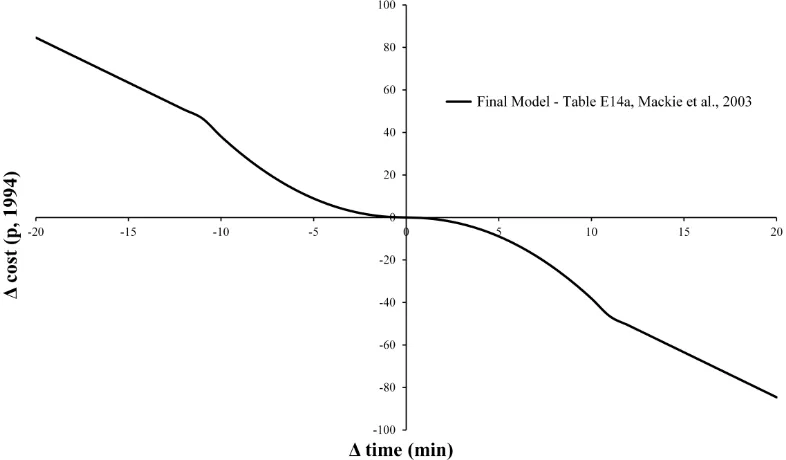
The 2001 Leeds ITS review drew similar conclusion as AHCG on the size effect, that VTTS is increasingly discounted below 10min. A “tapered” indifference curve was then estimated to represent the level of discount for time
[image:5.544.81.474.323.553.2]changes between a threshold θ, and was coined as “perception effect”. A grid search was undertaken to estimate the parameter θ and m, which were found to be 11 minutes and 2.09 respectively. The indifference curve for commuting trips that incorporates the “perception effect” is shown below:
Fig. 1. Indifference curves with perception effect (Mackie et. al, 2003)
3.2.3.Journey cost covariates
The recommended model by Leeds ITS in 2001 also includes continuous interaction between cost and the journey cost covariates income level and journey distance. The original idea was to isolate the “budget effects” on VTTS,
based on observations of coefficients in discrete segmentation that higher income households show much higher VTTS. In the actual formulation, current journey cost is used as proxy of journey distance since the SC experiment did not collect distance information. This elasticity model allows deterministic taste heterogeneity, which is not only desirable for interpretation issues but also could also be advantageous in model estimation to random coefficient approaches for large dataset (Hess et al., 2008). It appears that the only drawback is concerning the non-linearity that might cause model estimation issue.
4.Model Re-estimation
4.1.Methodology
A continuous MMNL model within a random coefficient framework was implemented in this research. This is not the only advanced choice model as there are a few other options that could be more desirable (e.g. latent class model, see Hess et al. (2011)). However, this continuous RCL model is the most commonly used advanced choice model for understanding taste heterogeneity (Hess, 2012). By implementing RCL, the VTTS valuation is estimated parametrically in this case. Alternatively, modeller could also estimate VTTS using a non-parametric approach, in which no specific distributional assumption on the random error term is made by making hypothesize that disturbances follow very general properties (Ben-Akiva and Lerman, 1985). This non-parametric procedure was applied in VTTS studies in Denmark and Sweden recently (Börjesson et al., 2012, Fosgerau, 2006, Fosgerau, 2007). One of the greatest benefits of non-parametric estimation is to ease the drawback from parametric analysis that misleading conclusions might be drawn when there is not enough data supporting the range of distribution (e.g. estimation primarily based on the tail of a distribution). However, non-parametric estimation is relatively cumbersome when the model specification includes several journey covariates simultaneously (Börjesson and Eliasson, 2014). Therefore, non-parametric estimation is not straight-forward for the VTTS valuation if we follow the model set out in Mackie et al. (2003) that includes both income and distance as journey cost covariates.
4.2.MMNL in preference space
4.2.1.Distributional assumptions
The pitfalls of incorporating inappropriate distributional assumptions of the random coefficients were discussed at length by Hensher and Greene (2003) and Hess et al. (2005). For VTTS valuation, the occurrence of counter-intuitive sign of the time or cost coefficients (i.e. positive sign) is problematic in particular as it contradicts to most economics theories. That being said, this is less of an issue for this research since VTTS is positive by design in the SC questionnaire by enforcing trading-offs of time and cost such that respondents could only choose between time increase or cost decrease (Bates and Whelan, 2001). This implies that time and cost coefficients must be negative, and hence any a priori statistical distributions that generate positive time or cost sensitivities must be rejected. Amongst the standard statistical distributions, lognormal and Johnson Sb are the best options to impose strict sign assumptions for the choice analysis. Nevertheless, standard normal, symmetrical triangular and uniform distributions for random coefficients were also tested to examine the sign of coefficients estimated. The distributional assumptions that were
applied in Biogeme (BIerlaire’s Optimization package for GEV Models Estimation) for this research are briefly
described below:
also lead to computational and model convergence issues (Hess et al., 2006); c, which is a draw from lognormal distribution can be expressed as:
Forߦ̱ܰሺߤǡ ߪଶሻǣ ܿ ൌ ݁క (6)
x Johnson Sb - it can be bounded and thus overcomes the long tail issue with lognormal distribution while maintaining the tight sign control; it is also the most flexible distribution in terms of the shape, which is controlled by 4 parameters in total (with two additional parameters for range and offset):
Forߦ̱ܰሺߤǡ ߪଶሻǣܿ ൌ ܽ ሺܾ െ ܽሻ ή
ାଵ (7)
Where c, a random draw from Johnson Sb distribution, is bounded between a and b (Hess et al., 2006)
x Normal - there is problem with the sign interpretation of the coefficients for unbounded distribution
x Uniform– specified with lower endpoint a and range parameter b; there might be sign issue when b is greater or equal to zero
x Symmetrical triangular - specified as summation of two uniform distribution; bounded to both side and hence avoid the long tail issue; sign issue when b is greater than zero
Unbounded distributions were not tested due to software limitation at the time of study. In terms of VTTS calculation, Monte Carlo simulation was required for most statistical distributions when both numerator and denominator are randomly distributed except for lognormal distributions. One million random Monte Carlo draws were assigned each time for computing the VTTS ratio. Since division between lognormal distributions results in a lognormal distribution, VTTS can be computed analytically (de Dios Ortúzar and Willumsen, 2011) instead of carrying out Monte Carlo simulation:
ܸܱ̱݈ܶ݃ܰ ൭ቆ൫௨ೣି௨൯ା
ೣమశమ
మ ቇǡ ݁ቆ൫௨ೣି௨൯ା ೣమశమ
మ ቇඥ݁ఙ௫మାఙ௬మሻ
െͳ൱ (8)
4.2.2.Model convergence issue
Another important consideration in RCL modelling is how many draws should be used in the simulation. Unfortunately there is no clear answer to this and the amount of draws required depends on dataset and model specification. It appears that at least 200 Halton draws should be set out as indicated by Chiou and Walker (2007). Multiple runs with different number of draws were undertaken to check the model convergence (i.e. stable Log-likelihood (LL) and VTTS) in this study.
Results of the model convergence assuming lognormal distribution for both time and cost coefficients are very worrying however as shown in Table 1. A range of draws from 100 to 1,250 Halton draws were used for this convergence test. It can be seen that this RCL model estimates a wide range of VTTS varying from 5.7p/min to 9.3p/min. Final LL estimates are relatively stable varying between -2,425 and -2,430, except for model run with 750 Halton draws that results in a LL of -2,456. Clearly, the model did not converge with 1250 Halton draws. It was also experienced that the Bison version of Biogeme could not complete any model runs with more than 1,250 Halton draws with this model specification. As such, model runs were undertaken using PythonBiogeme, which is a python version of Biogeme that allows parallel computing and more flexible model specification (Bierlaire and Fetiarison, 2009).
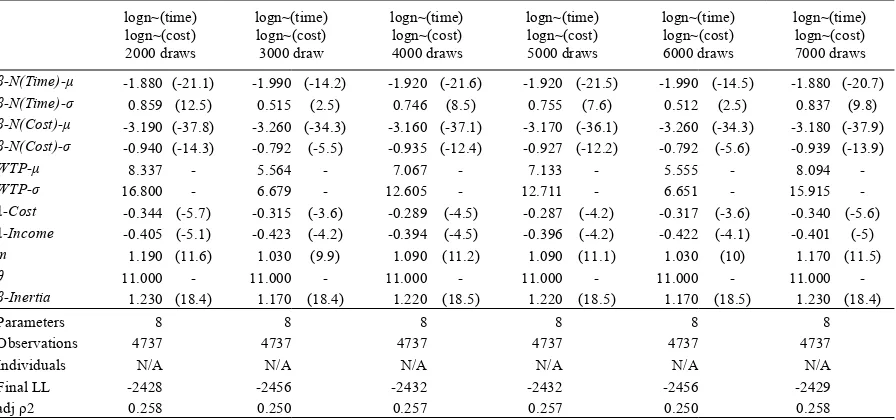
Table 2 shows that even pushing number of Halton draws from 2000 to 7000 using the PythonBiogeme, the RCL model with log-normally distributed random time and cost coefficients still could not converge as VTTS varies between 5.6p/min to 8.3p/min.
There is an interesting “cyclic” pattern emerged: LL’s are the highest with 4000 and 7000 draws and an average LL around -2,430 while VTTS estimates revolve around 7p/min to 8p/min. LL’s are the lowest with 3000 and 6000 draws and an average LL and VTTS at around -2,455 and 5.5p/min respectively. This problem could be related to the complicated non-linear formulation that produces log-likelihood functions which are not globally concaved. Amongst these model estimated using different number of draws, the lognormal RCL with 5000 draws was adopted as it results in fairly good LL at one of the LL “peaks” as well as a relatively averaged VTTS of 7.13p/min.
goodness-of-fit improvement comes at very high computing cost though. The model estimation for 100 Halton draws using Johnson Sb distribution was completed in 4.5 hours while it simply takes 3 hours only to estimate a lognormal RCL model with 1250 Halton draws. Also, attempts were made to add more draws for testing Johnson Sb distribution; however, model did not converge even after very long run time, revealing significant computational challenges in implementing Johnson Sb distributions for complex non-linear formulation.
Table 1. Model convergence test for RCL-Lognormal (100 to 1250 draws)
logn~(time) logn~(cost) 100 draws logn~(time) logn~(cost) 250 draws logn~(time) logn~(cost) 500 draws logn~(time) logn~(cost) 750 draws logn~(time) logn~(cost) 1000 draws logn~(time) logn~(cost) 1250 draws
β-N(Time)-μ -1.950 (-23.3) -1.810 (-21.5) -1.980 (-18.5) -1.970 (-12) -1.980 (-22.1) -1.850 (-21.6)
β-N(Time)-σ 0.888 (13) -0.664 (-8.6) -0.909 (-3.2) 0.471 (1.6) 0.987 (10.2) 0.677 (8.8)
β-N(Cost)-μ -3.230 (-38.9) -3.130 (-34.4) -3.210 (-35.2) -3.260 (-33.6) -3.220 (-36.6) -3.110 (-35.4)
β-N(Cost)-σ -1.030 (-12) 0.928 (14) 0.904 (9.2) -0.820 (-4.4) -0.998 (-11.3) -0.936 (-13.6)
WTP-μ 9.068 - 7.178 - 7.781 - 5.681 - 9.254 - 6.870 -
WTP-σ 20.986 - 11.744 - 15.896 - 6.830 - 22.991 - 11.492 -
λ-Cost -0.300 (-4.8) -0.334 (-5) -0.285 (-4.3) -0.311 (-3.3) -0.305 (-4.5) -0.316 (-5)
λ-Income -0.404 (-5.2) -0.409 (-4.7) -0.392 (-4.4) -0.433 (-3.9) -0.386 (-4.6) -0.398 (-4.2)
m 1.160 (11.1) 1.110 (11.5) 1.140 (9.1) 1.030 (9.6) 1.180 (11.3) 1.080 (11.4)
θ 11.000 - 11.000 - 11.000 - 11.000 - 11.000 - 11.000 -
β-Inertia 1.240 (18.5) 1.210 (18.5) 1.230 (18.1) 1.170 (18) 1.250 (18.4) 1.220 (18.4)
Parameters 8 8 8 8 8 8
Observations 4737 4737 4737 4737 4737 4737
Individuals 695 695 695 695 695 695
Final LL -2427 -2431 -2431 -2457 -2426 -2431
adj ρ2 0.258 0.257 0.257 0.249 0.259 0.257
Model estimations software: Bison Biogeme 2.2 (CFSQP)
Table 2. Model convergence test for RCL-Lognormal (2000 to 7000 draws)
logn~(time) logn~(cost) 2000 draws logn~(time) logn~(cost) 3000 draw logn~(time) logn~(cost) 4000 draws logn~(time) logn~(cost) 5000 draws logn~(time) logn~(cost) 6000 draws logn~(time) logn~(cost) 7000 draws
β-N(Time)-μ -1.880 (-21.1) -1.990 (-14.2) -1.920 (-21.6) -1.920 (-21.5) -1.990 (-14.5) -1.880 (-20.7)
β-N(Time)-σ 0.859 (12.5) 0.515 (2.5) 0.746 (8.5) 0.755 (7.6) 0.512 (2.5) 0.837 (9.8)
β-N(Cost)-μ -3.190 (-37.8) -3.260 (-34.3) -3.160 (-37.1) -3.170 (-36.1) -3.260 (-34.3) -3.180 (-37.9)
β-N(Cost)-σ -0.940 (-14.3) -0.792 (-5.5) -0.935 (-12.4) -0.927 (-12.2) -0.792 (-5.6) -0.939 (-13.9)
WTP-μ 8.337 - 5.564 - 7.067 - 7.133 - 5.555 - 8.094 -
WTP-σ 16.800 - 6.679 - 12.605 - 12.711 - 6.651 - 15.915 -
λ-Cost -0.344 (-5.7) -0.315 (-3.6) -0.289 (-4.5) -0.287 (-4.2) -0.317 (-3.6) -0.340 (-5.6)
λ-Income -0.405 (-5.1) -0.423 (-4.2) -0.394 (-4.5) -0.396 (-4.2) -0.422 (-4.1) -0.401 (-5)
m 1.190 (11.6) 1.030 (9.9) 1.090 (11.2) 1.090 (11.1) 1.030 (10) 1.170 (11.5)
θ 11.000 - 11.000 - 11.000 - 11.000 - 11.000 - 11.000 -
β-Inertia 1.230 (18.4) 1.170 (18.4) 1.220 (18.5) 1.220 (18.5) 1.170 (18.5) 1.230 (18.4)
Parameters 8 8 8 8 8 8
Observations 4737 4737 4737 4737 4737 4737
Individuals N/A N/A N/A N/A N/A N/A
Final LL -2428 -2456 -2432 -2432 -2456 -2429
adj ρ2 0.258 0.250 0.257 0.257 0.250 0.258
Model estimations software: PythonBiogeme 2.2 (CFSQP)
[image:8.544.52.500.381.591.2]series polynomial. Where more Legendre polynomials are added, the approximation is supposed to increase. Likelihood ratio tests were then carried out to test the base distribution against the generalized distribution. Results
[image:9.544.45.495.118.416.2]from SNP show that both the time and cost coefficients are the “true” mixing distributions in this case.
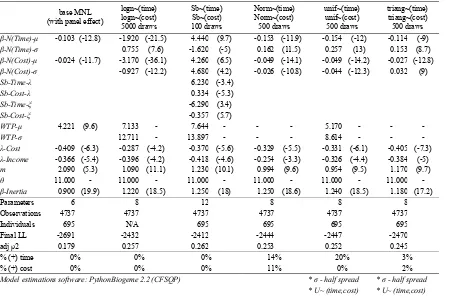
Table 3. MNL and MMNL model results in preference space
(with panel effect) base MNL
logn~(time) logn~(cost) 5000 draws
Sb~(time) Sb~(cost) 100 draws
Norm~(time) Norm~(cost) 500 draws
unif~(time) unif~(cost) 500 draws
triang~(time) triang~(cost) 500 draws
β-N(Time)-μ -0.103 (-12.8) -1.920 (-21.5) 4.440 (9.7) -0.153 (-11.9) -0.154 (-12) -0.114 (-9)
β-N(Time)-σ 0.755 (7.6) -1.620 (-5) 0.162 (11.5) 0.257 (13) 0.153 (8.7)
β-N(Cost)-μ -0.024 (-11.7) -3.170 (-36.1) 4.260 (6.5) -0.049 (-14.1) -0.049 (-14.2) -0.027 (-12.8)
β-N(Cost)-σ -0.927 (-12.2) 4.680 (4.2) -0.026 (-10.8) -0.044 (-12.3) 0.032 (9)
Sb-Time-λ 6.230 (-3.4)
Sb-Cost-λ 0.334 (-5.3)
Sb-Time-ξ -6.290 (3.4)
Sb-Cost-ξ -0.357 (5.7)
WTP-μ 4.221 (9.6) 7.133 - 7.644 - - - 5.170 - - -
WTP-σ 12.711 - 13.897 - - - 8.614 - - -
λ-Cost -0.409 (-6.3) -0.287 (-4.2) -0.370 (-5.6) -0.329 (-5.5) -0.331 (-6.1) -0.405 (-7.3)
λ-Income -0.366 (-5.4) -0.396 (-4.2) -0.418 (-4.6) -0.254 (-3.3) -0.326 (-4.4) -0.384 (-5)
m 2.090 (5.3) 1.090 (11.1) 1.230 (10.1) 0.994 (9.6) 0.954 (9.5) 1.170 (9.7)
θ 11.000 - 11.000 - 11.000 - 11.000 - 11.000 - 11.000 -
β-Inertia 0.900 (19.9) 1.220 (18.5) 1.250 (18) 1.250 (18.6) 1.240 (18.5) 1.180 (17.2)
Parameters 6 8 12 8 8 8
Observations 4737 4737 4737 4737 4737 4737
Individuals 695 N/A 695 695 695 695
Final LL -2691 -2432 -2412 -2444 -2447 -2470
adj ρ2 0.179 0.257 0.262 0.253 0.252 0.245
% (+) time 0% 0% 0% 14% 20% 3%
% (+) cost 0% 0% 0% 11% 0% 2%
Model estimations software: PythonBiogeme 2.2 (CFSQP) * σ - half spread * σ - half spread * U~ (time,cost) * U~ (time,cost)
Model results also indicate that parameter m, which controls the curvature of the VTTS “discount” for small travel
time savings, has dropped significantly from 2.1 in MNL to 1.1 and 1.2 in RCL-lognormal and RCL-Johnson Sb models respectively. By definition this mparameter becomes 1 when there is no VTTS “discount” at all. Table 4 and
[image:9.544.78.467.540.632.2]Figure 2 demonstrate the significant reduction of VTTS “discount” for travel time savings smaller than 11min. For instance, VTTS is estimated to be discounted by 58% at 5min time savings using basic MNL model but such reduction almost got completely wiped out to 7% only as estimated by RCL model. It implies that the size effect of VTTS is almost negligible in this setup, or is much smaller than what modellers used to think in the past using this AHGC dataset. Further research is required to investigate such reduced size effect.
Table 4. VTTS “discount” for small travel time savings
Time Savings
(min)
VTTS “Discount” Time
Savings (min)
VTTS “Discount”
MNL MMNL Lognormal (5000 Draws) MNL MMNL Lognormal (5000 Draws)
10 -10% -1% 5 -58% -7%
9 -20% -2% 4 -67% -9%
8 -29% -3% 3 -76% -11%
7 -39% -4% 2 -85% -14%
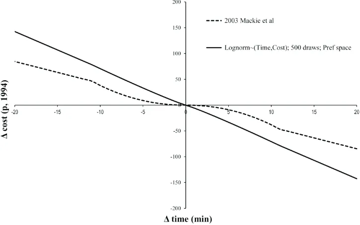
Fig. 2. Indifference curves with perception effect – MMNL (Lognormal, preference space) vs. MNL
5.Model Re-estimation
This study shows strong empirical evidence of taste variation amongst respondents, as exemplified by the improved LL and goodness-of-fit produced by RCL models. Rigorous tests have been undertaken to examine a range of possible high and low estimates of VTTS. This work recommends the RCL model with lognormal distribution assumed for time and cost coefficients in preference space, which produces good model fit yet providing more superior computing advantage over RCL model with Sb distributional assumptions. Hence, the recommended VTTS is 7.13p/min, which is 69% higher than the current official VTTS of 4.22p/min. A graphical representation of the VTTS changes in relation to journey cost and income is presented in Figure 3.
Fig. 3. (a) VTTS distribution for MNL; (b) VTTS distribution for MMNL – Lognormal-RCL
[image:10.544.59.461.437.612.2]The re-estimated VTTS for non-working trips presented in this paper is substantially different to the official VTTS estimated in the 2001. Therefore, it highlights the need to update the current appraisal VTTS using a more advanced choice model. Furthermore, with the VTTS estimated by RCL model now becomes a distribution itself, new modelling approach could better utilize this useful information. For instance, modellers can incorporate variation of taste amongst population through micro-simulation approach within an activity-based modelling framework or form very refined VTTS segmentation that closely resembles the VTTS distributional profile to provide more realistic modelling of travel behaviour, in particular for some pricing schemes in transport.
It is also shown that RCL model reduces the parameter m of the “perception effect” to almost one and hence significantly reduces the VTTS “discount” for small travel time savings. This finding challenges the need to reduce or even ignore the small travel time savings entirely for appraisal as in some countries like Germany. Lastly, the significant difference of VTTS outcomes resulted by varying model specifications, distributional assumptions and number of draws demonstrated in this study also encourages decision-makers to set out more stringent guidelines to ensure advanced choice modelling approaches adopted for appraisal evaluation are specified appropriately and applied consistently amongst choice modellers for fair assessment of travel benefits.
Acknowledgements
This paper is largely based on research conducted as part of my dissertation submitted for the MSc Transport Planning at the University of Leeds. I would like to take this opportunity to sincerely thank my supervisor Professor Stephane Hess for his support and guidance throughout this research. Any mistakes in the present paper remain the responsibility of the author.
References
Accent Marketing & Research and Hague Consulting Group [AHCG], 1999. The Value of Travel Time on UK Roads, Final Report for Department of the Environment, Transport and Regions, Netherlands, The Hague.
Algers, S., Bergström, P., Dahlberg, M., & Lindqvist Dillén, J., 1998. Mixed logit estimation of the value of travel time (No. 1998: 15). Working Paper, Department of Economics, Uppsala University.
Bates, J., Whelan, G., 2001. Size and sign of time savings. Working Paper 561. Institute of Transport Studies, University of Leeds. Beesley, M. E., 1965. The value of time spent in travelling: some new evidence. Economica, 174-185.
Ben-Akiva, M., Bolduc, D., 1996. Multinomial probit with a logit kernel and a general parametric specification of the covariance structure. Dʹepartement d'ʹeconomique, Universitʹe laval with Department of Civil and Environmental Engineering, Massachusetts Institute of Technology. Ben-Akiva, M. E., Lerman, S. R., 1985. Discrete choice analysis: theory and application to travel demand (Vol. 9). MIT press.
Bierlaire, M., Fetiarison, M., 2009. Estimation of discrete choice models: extending BIOGEME. In Swiss Transport Research Conference (STRC). Börjesson, M., Eliasson, J., 2014. Experiences from the Swedish Value of Time study. Transportation Research Part A: Policy and Practice, 59,
144-158.
Börjesson, M., Fosgerau, M., & Algers, S., 2012. Catching the tail: Empirical identification of the distribution of the value of travel time. Transportation Research Part A: Policy and Practice, 46(2), 378-391.
Chiou, L., Walker, J. L., 2007. Masking identification of discrete choice models under simulation methods. Journal of Econometrics, 141(2), 683-703.
Daly, A., Hess, S., Train, K., 2012. Assuring finite moments for willingness to pay in random coefficient models. Transportation, 39(1), 19-31. Daly, A., Tsang, F., Rohr, C., 2014. The value of small time savings for non-business travel. Journal of Transport Economics and Policy (JTEP),
48(2), 205-218.
De Borger, B., Fosgerau, M., 2008. The trade-off between money and travel time: A test of the theory of reference-dependent preferences. Journal of Urban Economics, 64(1), 101-115.
de Dios Ortúzar, J., Willumsen, L. G., 2011. Modelling transport. John Wiley & Sons.
Dillén, J. L., Algers, S., 1999. Further research on the national Swedish value of time study. In World Transport Research: Selected Proceedings of the 8th World Conference on Transport Research (No. Volume 3).
Fosgerau, M., 2006. Investigating the distribution of the value of travel time savings. Transportation Research Part B: Methodological, 40(8), 688-707.
Fosgerau, M., 2007. Using nonparametrics to specify a model to measure the value of travel time. Transportation Research Part A: Policy and Practice, 41(9), 842-856.
Fosgerau, M., Bierlaire, M., 2007. A practical test for the choice of mixing distribution in discrete choice models. Transportation Research Part B: Methodological, 41(7), 784-794.
Gunn, H., Burge, P., 2001. The value of travel time savings: some new evidence. Paper presented at the European Transport Conference, Cambridge, 10-13 September, 2001
Hensher, D. A., Greene, W. H., 2003. The mixed logit model: the state of practice. Transportation, 30(2), 133-176.
Hess, S., 2005. Advanced discrete choice models with applications to transport demand (Doctoral dissertation, University of London).
Hess, S., 2012. Rethinking heterogeneity: the role of attitudes, decision rules and information processing strategies. Transportation Letters, 4(2), 105-113.
Hess, S., Ben-Akiva, M., Gopinath, D., & Walker, J., 2011. Advantages of latent class over continuous mixture of logit models. Institute for Transport Studies, University of Leeds. Working paper.
Hess, S., Bierlaire, M., Polak, J. W., 2005. Estimation of value of travel-time savings using mixed logit models. Transportation Research Part A: Policy and Practice, 39(2), 221-236.
Hess, S., Erath, A., Axhausen, K. W., 2008. Estimated value of savings in travel time in Switzerland: Analysis of pooled data. Transportation Research Record: Journal of the Transportation Research Board, 2082(1), 43-55.
Hess, S., Polak, J. W., 2006. Distributional assumptions in mixed logit models. Transportation Research Board 85th Annual Meeting, 2006.
Kahneman, D., Tversky, A., 1979. Prospect theory: An analysis of decision under risk. Econometrica: Journal of the Econometric Society, 263-291.
Mackie, P. J., Wardman, M., Fowkes, A. S., Whelan, G., Nellthorp, J., & Bates, J. (2003). Values of travel time savings UK. Working Paper. Institute of Transport Studies, University of Leeds, Leeds, UK
McFadden, D., 1974. Conditional logit analysis of qualitative choice behavior. Frontiers in Econometrics, 105-142. McFadden, D., Train, K., 2000. Mixed MNL models for discrete response. Journal of applied Econometrics, 15(5), 447-470. MVA, ITS and TSU, 1987. The Value of Travel Time Savings, Policy Journals, 1987
Nellthorp, J., Sansom, T., Bickel, P., Doll, C., & Lindberg, G., 2001. Valuation conventions for UNITE, UNITE (UNIfication of accounts and marginal costs for Transport Efficiency), 5th Framework RTD Programme. ITS, University of Leeds, Leeds.
Stathopoulos, A., Hess, S., 2012. Revisiting reference point formation, gains–losses asymmetry and non-linear sensitivities with an emphasis on attribute specific treatment. Transportation Research Part A: Policy and Practice, 46(10), 1673-1689.
Train, K. E., 2009. Discrete choice methods with simulation. Cambridge university press.
Revelt, D., Train, K., 1998. Mixed logit with repeated choices: households' choices of appliance efficiency level. Review of economics and statistics, 80(4), 647-657.
Revelt, D., Train, K., 2000. Customer-specific taste parameters and Mixed Logit: Households' choice of electricity supplier. Department of Economics, UCB.
Van de Kaa, E. J., 2005. Heuristic Judgement, Prospect Theory and Stated Preference Surveys Aimed to Elicit the Value of Travel Time. In European Transport Conference, 2005.
Walker, J. L., Ben-Akiva, M., 2011. Advances in discrete choice: mixture models. A Handbook of Transport Economics, 160.