Prawn trawl shape due to flexural rigidity and hydrodynamic forces

(1)

Prawn Trawl Shape due to

Flexural Rigidity and

Hydrodynamic Forces

By

Cheslav Balash

B.Eng (Hons) Kaliningrad State Technical University, Russia (1999) M.Eng. Memorial University of Newfoundland, Canada (2008)

Submitted in fulfilment of the requirement for the degree of Doctor of Philosophy at the University of Tasmania

(2)

Declaration of Originality

(3)

i

Abstract

Energy efficiency and ecological sustainability have become vital issues for the Australian and global prawn fisheries. The scientific community and innovative industry operators have introduced fishing gear modifications for drag and unwanted catch reduction. This project has investigated the potential for further drag reduction, focusing on the extent to which prawn net flexural rigidity affects the drag.

A novel experimental technique was developed to quantify flexural rigidity for nets. The concept of the technique was to measure the mesh opening under various loads applied in longitudinal and transverse directions. A relative difference between values showed a resistance of the mesh to bend, and the results were fitted into an existing analytical solution. The geometric parameters of nets were measured applying a digital photogrammetric method.

(4)

ii

Acknowledgments

(5)

iii

List of Figures

Fig.1.1 The geography of prawn harvesting in Australia according to the

Australian Council for Prawn Fisheries

(www.prawncouncil.com.au). Each Australian prawn fishery has been marked with a prawn – it can be seen that prawn fisheries are extended across Australia……….. 2 Fig. 1.2 Resistance components of a 22m LWL Success class trawler

operating at 3 knots with double-rigged 6 fathom nets (FRDC Workshop

2005)…………... 3 Fig. 1.3 Prawn trawl system components………. 5 Fig. 1.4 A schematic example of a prawn trawl (above); and examples of

body and wing tapers (below). P – Point, M – Mesh, B –

Bar………... 6

Fig. 1.5 Four prawn net designs traditionally used by trawl operators in Australia…... 8 Fig. 1.6 Schematic illustration of twine area reduction for double and

triple rigs; a similar situation occurs for quad and quintuple rigs... 10 Fig. 1.7 Tongue prawn trawl design………. 11 Fig. 1.8 A prawn trawl tested in a flume tank (Flesser, 1994). The net

wrinkling, especially in the aft part of the trawl, can be clearly

seen………. 14

Fig. 1.9 Definition of angle of an attack α between the net and incoming

flow………. 16

Fig. 1.10 Drag coefficient for prawn trawls of equal design and different netting material (spectra and polyethylene). Sea-trials data for a

constant towing speed of 1.6m/s (Lowe,

1996)………... 17

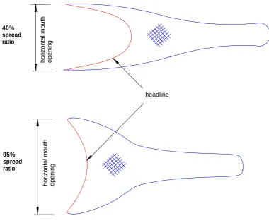
Fig. 1.11 The schematic examples of the netting part with 40% and 95% spread ratio. The spread ratio is defined as the percentage of the headline to the horizontal spread……….... 18 Fig. 1.12 Drag coefficient vs. net solidity for knotted and knotless plane

(9)

vii

Fig. 1.13 Drag coefficient for knotted net vs. knotless net according to empirical formulae by Milne (1979)………... 20 Fig. 2.1 A sample of braided twine………... 22 Fig. 2.2 A sample of twisted twine………... 22 Fig. 2.3 The approximation of the knot size and shape by Fridman

(1973)…………... 23 Fig. 2.4 The areas covered by the knots (Klust (1982), Fig. 33)………... 23 Fig. 2.5 The Otsu’s (1979) method threshold application in Matlab for a

mosquito screen (image is enlarged)………..…………. 24 Fig. 2.6 Idealized mesh grid………... 24 Fig. 2.7 The outside perimeter (edge detecting) of a mosquito

screen……… 25

Fig. 2.8 Idealized mesh sketch………... 25 Fig. 2.9 The effect of mesh number per image on solidity error for three

types of solidity (low, average and high)……….... 27 Fig. 2.10 The logarithmic representation of Fig. 2.9………... 28 Fig. 2.11 The error in the drag coefficient for plane nets produced by an

error of 0.1% on net solidity and an error of 1% and 5% in twine

thickness……….. 30

Fig. 2.12 Twine thickness obtained by measurements with vernier callipers

and image analysis………... 30

Fig. 2.13 Mesh orientation specification……… 31 Fig. 3.1 Mesh geometry specification……….. 34 Fig. 3.2 Plane net under the uniform load considered by Baranov

(1960)……… 34

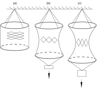
Fig. 3.3 A net sample attached to two hoops………... 35 Fig. 3.4 A net attached to the hoops in transverse mesh orientation:

(a) with no load applied (the weight of the net and the bottom hoop only); (b, c) the net acquires an hour-glass shape as the load

gradually increases……….. 36

(10)

viii

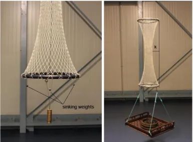
Fig. 3.6 A net restrained between the hoops - experimental set-up: (a) a light polyethylene pipe hoop on the left, (b) and aluminium

hoops on the right)……….. 38

Fig. 3.7 Nylon samples in the longitudinal orientation attached to 1m diameter hoops with the horizontal mesh hanging coefficient of 0.32 and 0.44 (eq. 4.8 and Table 3.1). As seen, the distance between the hoops does not significantly change with hanging

coefficient variation……… 40

Fig. 3.8 An example of calculated net shape using numerical method of Prior (2001)……… .

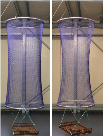
42 Fig. 3.9 Transversely-oriented net sample under various loads. As the

load increases, the shape of the system gradually acquires an

hour-glass……… 43

Fig. 3.10 _{Mesh resistance to stretch in the transverse direction for three}

samples (Table 2.1). A mesh opening coefficient (y-axis) is the ratio of mesh opening in the longitudinal orientation to mesh opening in the transverse orientation……….. 44 Fig. 3.11 Flexural rigidity as a function of twine linear density: data from

Sals et. al (2007) (blue dots), and present study (red dots)……… .

47 Fig. 3.12 Flexural rigidity as a function of twine linear density: averaged

flexural rigidity data point for every sample from Sals et. al

(2007) and present study………. 48

Fig. 4.1 (a)

Net plan for ¼ scale 8 fathom Florida Flyer for all samples except Hampidjan Dynex (Table 2.1) Taper sequences are on the left side of the plan, and numbers of meshes corresponding to these tapers are on the right. Top and bottom panels are symmetric. P – Point, M – Mesh, B – Bar (definition is provided

in section 1.3)……….. 51

Fig. 4.1 (b)

Net plan for ¼ scale 8 fathom Florida Flyer for the Hampidjan Dynex model (Table 2.1)………..…….. 52 Fig. 4.2 Model attached to trawl evaluation rig and placed in the

mid-stream……….. 53

Fig. 4.3 A sample of flow distribution in a flume tank cross-section (Kok, 2010); the legend bar shown on the right presents flow speed in

m/s………... 55

(11)

ix

Fig. 4.5 Force vector breakdown………... 59

Fig. 4.6 Trawl shape captured with side view and top cameras………... 62

Fig. 4.7 A camera calibration frame (top view)……….. 63

Fig. 4.8 (a) Samples of raw data: continuously-recorded drag measurements for four sets of flow speed and transient (decelerating) flow regimes. (b) Samples of raw data: net drag in correspondence to these four velocities with 300 time points only for each set………... 64

Fig. 4.9 Propellers’ performance: #1 and #2 on top, #3 and #4 on bottom………. 67

Fig. 4.10 Net drag vs. flow velocity (L – pre-stretched longitudinally, T – transversely)……… 68

Fig. 4.11 Drag residual distribution………... 69

Fig. 4.12 Drag vs. flow velocity – averaged values………... 69

Fig. 4.13 A sample of error bars with 99% confidence……….. 69

Fig. 4.14 Drag vs. velocity – a power exponent is adjusted to the figure of 2. A drag difference between transverse (T – red dots) and longitudinal (L – blue dots) pre-stretch increases for a given sample as the model stiffness increases……….. 71

Fig. 4.15 A relative drag increase between two types of pre-stretch (L and T) due to a change in netting stiffness……….... 72

Fig. 4.16 Drag coefficient with respect to Reynolds number………... 74

(12)

x

List of Tables

Table 1.3 Various reports on parameters that determine the drag coefficient of the plane net at a low angle of attack (Re is Reynolds number, Sdis netting solidity (blockage) and α is

an angle of attack)………. 15

Table 2.1 Net geometry………. 31

Table 3.1 A number of meshes attached to the hoop and corresponding hanging coefficient (eq. 4.8) for four nylon

samples……… 39

(13)

xi

Nomenclature

a longitudinal dimension of a knot Amesh mesh area

Aout image area (outline area)

Aporous porous area of net

b transverse dimension of a knot c circumference

out net D

C [ ] the drag coefficient for the net as a function of the outline area ]

[cyl D

C drag coefficient for the circular cylinder E modulus of elasticity

f twine bar tension Fd drag force

Fin in-pull force

Fr Froude number

g acceleration due to gravity,. I second moment of inertia L characteristic trawl length m mesh bar

n number of meshes Ne Newton’s number

P outside mesh perimeter

q static force generated by rigging r radius

Re Reynolds number

R-tex linear density of the netting yarn or twine

Sd netting solidity (bloackage)

T frameline tension U flow velocity

ux horizontal hanging coefficient

Uy Vertical hanging coefficient

α incident angle between the flow and net

γ*

(14)

xii ρ water density

(15)

1

Chapter 1

1. Introduction

This chapter highlights engineering challenges that prawn fisheries presently face. The picture is given in an Australian context, but similar difficulties are experienced in other prawn fishery regions of the world. Project objectives and long-term goals are then formulated; followed by the reviews that familiarise the reader with the background of the project:

 An overview of prawn trawl systems is provided along with the reasons for selecting a prawn trawl design as a case study for the current project.

 Shortcomings of the trawl scaling practices are discussed.

 Drag variables specific to prawn and fishing nets and trawls are discussed.

1.1 Current needs for Australian prawn fisheries from an engineering perspective

(16)

2

that the research of the prawn industry was primarily focused on environmental issues, but not industry efficiency. Recent research within the prawn industry has primarily focused on by-catch reduction, prawn behaviour and effects of prawn trawling on the seabed with little attention given to gear design. However, gear modifications may not only improve fishery profitability, but maximize effects on ecological sustainability.

Fig. 1.1 Prawn harvesting in Australia according to the Australian Council for Prawn Fisheries (www.prawncouncil.com.au). Each Australian prawn fishery has been marked with a prawn – it can be seen that prawn fisheries are extended across Australia.

Too often, solutions based on gear modifications are overlooked, and operationally-based changes are implemented instead. This practice impedes the evolution of the gear, and moreover, represents an example of not addressing the source of the problem. For instance, trawl design modifications can greatly reduce the amount of trawl by-catch caught, but the selectivity issue has been seen as largely solved since the introduction of the compulsory use of Turtle Exclusion and By-catch Reduction Devices.

[image:16.595.186.476.216.426.2]

(17)

3

2008) summarised major operational and technical approaches to reduce fuel expenses. Drag force reduction technologies (i.e. skin coatings and naval stabilisers) were suggested as one of the major factors for higher energy efficiency. Fishing gear modification also retains a great potential for drag force reduction. As can be seen from Fig. 1.2, nets and wires can produce up to 2/3 of the total drag whilst trawling.

Fig. 1.2 Resistance components of a 22m LWL Success class trawler operating at 3 knots with double-rigged 6 fathom nets (FRDC 2005).

Trawl gear is flexible and its final shape whilst trawling is often unknown. To be able to predict its shape, prior knowledge is required of how inertial, viscous and gravitational forces impact on the load distribution through the net. Once understood better, then these net shape predictions will allow a more detailed assessment of the selectivity and seabed impacts of the net.

The establishment of the relationship between trawl shape and forces may allow the production of a net design with lower water resistance. Such new net modifications should promote better flow throughout the trawl and could inform researchers and off-shore operators for optimal selectivity. In addition, a better knowledge of trawl shape and nearby water flow will enhance trawl gear development and operation, and provide the industry more confidence to participate in gear development processes.

2% 5%

31%

62%

(18)

4

1.2 Aims and goals

The ultimate project goal is to address the issues of trawl selectivity and energy efficiency through designing a prawn trawl of low drag and minimised ecological footprint.

The following major objectives are addressed within this thesis:

 To develop a tool for trawl shape measurement in conjunction with applied loads.

 To develop a method for quantifying fish net flexural rigidity (stiffness), and to estimate flexural rigidity figures for conventional and innovative prawn nets.

 To quantify the extent by which net flexural rigidity affects prawn trawl drag.

 To establish a technique allowing prawn full-scale netting material usage in model experiments.

 To estimate by what extent the Reynolds number, net porosity and an angle of incident flow determine the drag coefficient for nets at a low angle of attack in application to prawn trawls.

The achievement of the above objectives will advance the knowledge of fishing net hydrodynamics, and coupled with practices will provide a methodological foundation for designing an optimal prawn trawl system of minimum drag force and optimal selectivity.

1.3 Overview of prawn trawl systems

Prawn trawl designs

(19)

5

and stimulates prawns to jump from the seabed as the trawl is towed through the water. The short vertical connection-chains allow the trawl’s bottom net panel to be just clear of the seabed, which minimizes the catch of seabed objects, including sessile benthic animals, and also prevents some net damage.

Fig. 1.3 Prawn trawl system components (redrawn from Sterling (1996).

(20)

6

1P3B body taper

1M3B wing taper 3Bars

1Point 3Bars

1Mesh

Fig. 1.4 A schematic example of a prawn trawl (above); and examples of body and wing tapers (below). P – Point, M – Mesh, B – Bar.

(21)

7

Various prawn trawl designs have been developed and utilized across the world. Even within the same country, prawn trawl designs vary from region to region. For example, Watson et al. (1984) conducted a review of various shrimp trawl designs employed in Southeastern United States waters. In Australia four basic designs are most commonly used: Florida Flyer, Sandakan, Gundry and Seibenhauser (Fig. 1.5). Florida Flyer is comprised of a combination of wing tapers, which provides a series of catenaries, while Gundry is typically of one type of a wing taper. Both designs, Florida Flyer and Gundry, often do not have side panels as wide wings provide a high enough vertical trawl opening. Sandakan being a simplified version of Florida Flyer has a lower number of taper sequences in the net mouth, but because of its narrow wings, side panels are required to satisfy the desired vertical trawl opening of about 1m. Seibenhauser has a cut of bars only in the mouth and it is comprised of wide side panels.

Thus, generic features of all four trawls would include:

 A wide wing or a side panel

 A series of two or three wing tapers

(22)

8

FLORIDA FLYER SANDAKAN

a sequence of wing tapers

no side panels, but wings are wider

with side panels and wings are shallow

GUNDRY

a steep wing taper

no side panels, but wings are wider

SEIBENHAUSER

wide side panel

a cut of bars only across the mouth

Fig. 1.5 Four prawn net designs traditionally used by trawl operators in Australia.

Drag saving technologies

(23)

9

linearly correlated with twine area reduction. Sterling (1996) showed that a triple rig provides about a 50% drag reduction compared to the single rig. The nature of drag saving produced with multiple rigs is not solely due to twine area reduction but due to redistribution of the otter board drag required to spread the trawl. In addition to the double and triple rigs shown in Fig. 1.6, the industry also employs quad and five rigs. However, besides drag saving benefits, fishermen need to consider operational implications of using multiple rigs. For example, as the quad rig is a system of two independent double rigs, uneven gear tension distribution caused by the rough sea-bed are more likely to occur while trawling the quad rig, which may lead to netting damage or even to the vessel being capsized.

A more recent innovation to significantly reduce drag was high-strength Dyneema® and spectra netting materials that allow the use of thinner twine compared to traditional materials. Small diameter Dyneema® and spectra netting twine are of similar breaking strength to traditional material, but the thinner twine results in decreased drag. However, a disadvantage of the new material is that it is significantly more expensive than the conventional netting, which makes trawl operators reluctant to widely implement the innovation. In addition, Dyneema® twine has very low bending stiffness, which produces operational difficulties due to fouling during trawl deployment and hauling.

A pleated-panel trawl built with square-mesh orientation in the side sections (described by Wray (1990) requires less force to spread the trawl as the tension is distributed more directly through the trawl along the square-mesh bars to the otter boards as opposed to a conventional diamond orientation where the tension tends to run to the bosom of the trawl and then to the otter boards along the frame lines. However, for a pleated trawl, a greater amount of twine is perpendicular to the flow because of its mesh orientation, which increases the netting drag and hence negates the benefits of a lower in-pull force.

(24)

10

square-mesh orientation in the top and bottom panels of the trawl, but not in side sections as in the pleated trawl. The square mesh panels are expected to focus the tension in the trawl towards the tongues, and ease the load on the otter boards, hence making the trawl easier to spread and minimise drag as smaller otter boards would be required.

single 24 fathom net

2 x 12 fathom double rig

3 x 8 fathom triple rig

single trawl

double rig - 50% of twine reduction

triple rig - 67% of twine reduction

(25)

11

TONGUE TRAWL

a 'tounge' shape of the top panel

bottom panel similiar to that of Sandakan design

Fig. 1.7 Tongue prawn trawl design.

1.4 Overview of trawl modelling practices

To study a physical phenomenon, analytical, numerical and experimental methods are applied. In application to fishing gear, due to hydro-elastic coupling, establishing and solving equations are possible for simplified cases only (Rozenshtein 2000).

An experimental study can be conducted at model or full-scale. Full-scale experiments at sea ensure the inclusion of all factors influencing the process. However, every run is impacted by secondary factors which are uncontrolled and arbitrary (currents, waves, wind, and uneven sea-bed). In model experiments, a studied process commonly has to be simplified with certain assumptions which may produce an error. However, the model experiments eliminate the noise effect of the environment and they are also more economical.

Initially a relation between experiments at model and full-scale was suggested by Tauti (1934). According to his theory, the drag force is assumed to be proportional to the square of the water velocity U (eq. 1.1):

2 ~U

(26)

12

Chow (1969) and Hu et al. (2001) applied the law to model mid-water trawls at a number of scales. The comparisons with full-scale showed a 50-70% drag force over prediction. The modelling rules were modified; however, those modifications are only applicable for the specific case studied. Fiorenti et al. (2004) also applied Tauti’s law for bottom trawls and found a large difference in drag between full-scale and model values. When Tauti’s law is applied for model testing, a high drag over prediction occurs as the drag coefficient is assumed to be constant between the model and prototype while it is often not the case.

Dikson (1961) proposed to use the Froude number for scaling:

U Fr

gL

 _1.2

where U is the flow velocity, g is the acceleration due to gravity, and L is a characteristic trawl length.

A recent application of Dickson’s approach (Hu et al. 2001) showed a significant divergence in the drag force between full-scale and model values as for Tauti’s method. Applying the Froude number as a condition of dynamic similarity assumes that the net is a solid three-dimensional body, but it is a porous two-dimensional surface (O'Neill, F.G. 2003). Instead O’Neill proposed to use twine thickness d, not trawl length L, as a geometric parameter for the Froude number; and the Reynolds number incorporated the trawl length. It was modified as follows to satisfy the similarity between inertial and viscous forces:

L Ud R_e



2

 1.3

(27)

13

Fridman (1973) conducted a dimensional analysis and recommended similarity criteria for fishing gear. The Froude number was modified as a ratio of the hydrodynamic forces to buoyancy forces:

2

*

U Fr

L





 1.4

where ρ is the water density, γ*is the volumetric weight which is a ratio of the netting weight in the water and the volume.

It was shown that for a Froude number above 130, which is a common case, the effect of buoyancy forces on the shape is not significant (Fridman, AL 1973). The Reynolds number was assumed to have a negligible effect on the drag coefficient for model experiments conducted in the subcritical flow regime. Dynamic similarity was proposed by keeping the ratio of static (generated by rigging) and hydrodynamic forces constant, namely Newton’s number:

2 2

U L

q Ne



 1.5

where q are the static forces generated by rigging.

(28)

14

material may be impractical if mechanical forces dominate over hydrodynamic forces, and thus, the obtained data is inaccurate. Flesser (1994) studied the effect of selvage tapers on the engineering performance of the Florida Flyer by testing full-scale trawls in a flume tank. The obtained data seems to be inconsistent, which was explained by ‘the wrinkle effect’ (Fig. 1.8). The problem occurred due to the hydrodynamic force being too low to overcome net stiffness and to enable the trawl to gain a proper shape.

[image:28.595.144.517.443.662.2]

The relation of hydrodynamic forces and net stiffness has not been largely addressed. Christensen (1975) considered stress-strain characteristics for fishing net modelling, but in respect to net material only. However, hydrodynamic forces are coupled to structural forces, and hence the relation of the former and the latter has to be established for accurate modelling. Tsurkov et al. (2011) experimentally estimated the drag for copper alloy nets. Their comparative analysis with previously published formulae on nylon net drag coefficient led to the conclusion that net flexibility should not be assumed negligible for quantifying the net drag coefficient.

Fig. 1.8 A prawn trawl tested in a flume tank (Flesser 1994).

(29)

15

1.5 Prawn trawl drag variables

As mentioned above, there is a non-linear relationship between trawl shape and hydrodynamic forces. Thus, to study a relation between net stiffness (shape) and hydrodynamic forces, it is initially necessary to consider the specific prawn trawl parameters which impact the drag force. According to hydrodynamic theory (Morison’s eq.) (Fredsøe & Sumer 1997), the drag force is proportional to the flow velocity squared and the cross-sectional area, provided the drag coefficient is independent of the Reynolds number. This is valid for solid bodies as their shape remains constant; the orientation of the body is the only other concern. A net is a system with multiple degrees of freedom which undergoes large deformation under external and internal forces. A prawn trawl represents a complex engineering structure, due to the structural compliance of the netting. The net changes its shape under the load, but as the shape changes, the loads are also changing, so there is a strong compliance coupling with hydrodynamic forces.

Angle of incident flow, net porosity and Reynolds number.

Table 1.1 Various reports on parameters that determine the drag coefficient of the plane net at a low angle of attack (Re is Reynolds number, Sd is netting

solidity (blockage) and α is an angle of attack).

Study Parameters

considered

Parameters affecting the drag coefficient Taniguchi (1968) Re, Sd=const, α =const Re

Dvernik (1971) Re, Sd, α α

Aarnes et al. (1990) Sd, α Sd, α

Buxton & DeAlteris (1993) Re, Sd, α =const Sd

Gjøsund & Enerhaug (2010) Re, Sd, α =const Re, Sd

(30)

16

diameter. Netting solidity Sd is the ratio of twine area and overall area covered

by the net. Netting porosity is the ratio of twine-free area and overall area covered by the net. As both parameters, netting solidity and porosity, quantify a relative net blockage area, they are interchangeably used in the literature.

flow

net angle of

attack

Fig. 1.9 Definition of angle of an attack α between the net and incoming flow.

(31)

17

solidity. Both studies showed that for cases of the Reynolds number being below

103, the Reynolds number significantly affects the net drag coefficient, in a trend

similar to what occurs for circular cylinders. However, the dependence of the drag coefficient on the Reynolds number for the net at a low angle to the flow remains inconclusive.

Netting material

Lowe (1996) investigated the drag saving potential for Spectra netting compared with polyethylene netting prawn trawls. Spectra permits higher breaking strength, so for similar breaking strength, 49% thinner twine was used to build spectra trawls. Twine reduction visibly resulted in a decrease in the drag force. However, in a non-dimensional form, as can be seen in Fig. 1.10, the drag coefficient for spectra netting is on average 10% higher compared to polyethylene; it varies 3-14% depending on the spread ratio. The drag variability could occur due to different material stiffness. Additionally, Balash et al. (2009) studied the drag force on plane netting samples and a similar tendency was detected. However, since construction properties of netting (twisted or braided) were not considered, it remains inconclusive to what extent netting material affects the drag coefficient. In addition, even though an allowance for knotted netting was incorporated through the net solidity, but knots might also affect the elastic properties of netting.

Fig. 1.10 Drag coefficient for prawn trawls of equal design and different netting material (spectra and polyethylene). Sea-trials data for a constant towing speed

of 1.6m/s (Lowe 1996).

0 0.1 0.2 0.3 0.4

0.40 0.50 0.60 0.70 0.80 0.90

Dr

a

g

co

e

ff

ici

e

n

t

Spread ratio, %

(32)

18

Horizontal trawl spread

Wakeford (1994) examined the effect of prawn trawl design features on the engineering performance which included, but was not limited to dependence of the drag force on the spread ratio. The spread ratio is defined as the percentage of the net spread to the headline (Fig. 1.11). The study determined optimal spread ratios for prawn trawls of different frame line taper sequences. It also quantified the dependence of the drag coefficient on the spread ratio for the selected trawl designs.

headline

ho

rizo

nt

al

mo

uth

op

en

in

g

ho

rizo

nt

al

mo

uth

op

en

in

g

40% spread ratio

[image:32.595.143.524.282.598.2]

95% spread ratio

Fig. 1.11 The schematic examples of the netting part with 40% and 95% spread ratio. The spread ratio is defined as the percentage of the headline to the

(33)

19

Knots

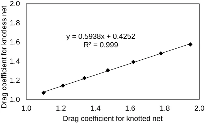
Baranov (1960) reported that knots have a negligibly small effect on the drag coefficient, similar to the effect of the intersecting points in knotless nets. However, Milne (1979) experimentally derived formulae for the drag coefficient of plane nets in a steady current specifically for knotted and knotless netting. As can be seen from Fig. 1.12 and Fig 1.13, the discrepancy in the drag coefficient between knotted and knotless nets linearly increases as net solidity increases (from 3% to 20%). As knot size is primarily a function of twine thickness, it is reasonable to assume that Milne considered the effect of knots on the drag coefficient by accounting extra solidity produced by knots. In experiments with plane nets, samples have to be restrained in a frame. Thus, if knots affect the drag force not only by increasing solidity, but by impacting the net shape, the effect would not be significant enough to be noted in the plane nets experiments. Trawls, however, are only restrained to a certain extent in their forepart by using otter boards to spread their opening. Tait (1987) conducted full-scale experiments at sea to investigate the effect of knots on the drag force of demersal (bottom) trawl nets. An average drag reduction of 12% for knotless trawls was found. However, the twine thickness for knotless and knotted trawls was not exactly equal. There is no evidence in the paper that the allowances were made for this difference. Thus, it remains uncertain to what extent knots contribute to the drag force.

Summary

Summarizing, the following parameters impact the drag force of trawls (in addition to those inherent for solid bodies):

 netting material;

 netting construction properties (braided or twisted);

 the knot factor (knotless or knotted netting);

 net design (sequence of tapers);

 trawl spread ratio.

(34)

[image:34.595.148.483.358.559.2]

20

Fig. 1.12 Drag coefficient vs. net solidity for knotted and knotless plane nets according to empirical formulae by Milne (1979).

Fig.1.13 Drag coefficient for knotted net vs. knotless net according to empirical formulae by Milne (1979).

0.00 0.50 1.00 1.50 2.00 2.50

0% 10% 20% 30% 40%

Dr a g co e ff ici e n t

Net blockage, %

Knotted net Knotless net

y = 0.5938x + 0.4252 R² = 0.999

1.0 1.2 1.4 1.6 1.8 2.0

Dr a g co e ff ici e n t fo r kn o tle ss n e t

(35)

21

Chapter 2

2. Net geometry estimation

This chapter reviews existing methodologies for twine geometry measurements. Given results’ uncertainty from these methods, a photogrammetric technique was developed in this study, and results for four nets commonly used by the industry are presented. The error in the drag coefficient due to the error in net porosity and twine diameter were also estimated.

2.1 Overview of existing techniques

Fishing gear, and prawn trawls in particular, are mainly constructed out of textile netting. As shown in Fig. 1.2, in prawn trawls, during trawling the netting is responsible for on average 2/3 of the total water resistance from the boat and gear. Hence, accurate net geometry estimation is crucial for drag force prediction. Various techniques have been developed by researchers and fishermen to estimate twine thickness, mesh and knot size.

(36)

22

Twine manufacturers commonly provide the R-tex number or the Runnage. The R-tex is the linear density of the netting yarn or twine in grams per kilometre

(Fridman 1986). Alternatively, R-tex can be represented through the Runnage (meters per kilogram). The diameter then can be estimated from eq. 2.1:

0.5

( )

1000

DT

t

Rtex d K

K

 2.1

where d is the twine diameter, KDT and Kt are empirical coefficients (the

coefficients are dependent on the netting material). For a given material, they vary by about 30% due to variation in construction properties, and thus the actual and calculated diameters may significantly differ.

Special gauges of various configurations have also been designed. Such gauges can be used for netting made from firm and braided twines only (Fig. 2.1) as the method does not allow estimating effective diameters of twisted twines (Fig. 2.2).

Fig. 2.1 A sample of braided twine.

Fig. 2.2 A sample of twisted twine.

(37)

23

approximate. Fonteyne et al. (2007) performed a comprehensive review of the existing methodologies and their shortcomings.

Fig. 2.3 The approximation of the knot size and shape by Fridman (1973).

Fig. 2.4 The areas covered by the knots (Klust 1982), Fig. 33).

Fridman (1973) approximated the knot as twine over which other twine is wound (Fig. 2.3). Klust (1982) estimated the knot sizes by applying a photographic method. As can be seen from Fig. 2.4, the knot size may depend greatly on the construction properties of netting. The samples a and c are made of the same material (polyamide), but one is twisted and another is braided. Both samples are of similar twine thickness, but knot sizes differ greatly.

2.2 The photogrammetric technique for netting porosity estimation

(38)

24

Conceptually, the code compares the number of pixels associated with the object (netting) to the number of remaining pixels (background).

There has been a significant amount of research conducted to develop techniques for distinguishing an object from the background. Pixels have to be classified as dark and light to distinguish dark objects from a light background (or vice versa). It is necessary to determine an optimal pixel classification (threshold) so a pixel belongs to the correct group (object or background). Extensive surveys of those techniques were performed by Weszka & Rozenfeld (1978). Otsu (1979) suggested a simplistic method of the threshold corresponding to the minimum sum of weighted-group variances. This is equivalent to selecting a threshold that minimizes the squared difference between the group means. This approach provides an optimal and automatically-selected threshold. It was implemented here in Matlab with the graythresh function. The example of this function application is presented in Fig. 2.5.

Fig. 2.5 The Otsu’s (1979) method threshold application in Matlab for a

mosquito screen (image is enlarged).

Fig. 2.6 Idealized mesh grid.

(39)

25

calculated by applying the bwarea function which estimates the number of on pixels in a binary image.

The total area was calculated by the multiplication of the image dimensions:

[x,y] = size(img)% image dimensions

Aout = x*y% projected area (total image area)

The twine area was found from the difference between the total and the porous area:

A = Aout-Pr% twine area

As can be seen from Fig. 2.6, the mesh bar m can be found as follows:

4 4

2 m mn

n m P

A_porous



 2.2

where Aporous is porous area, P is outside mesh perimeter and n is a number of

meshes. To estimate the perimeter, the bwperim function was used, which ultimately detects the edges of the object (Fig. 2.7) and counts a pixel as a part of the perimeter if it is non-zero (black) and connected to at least one zero-valued pixel (white).

Fig. 2.7 The outside perimeter (edge detecting) of a mosquito screen.

Fig. 2.8 Idealized mesh sketch.

(40)

26 2 2 ) ( 2 d m d md A A S out d _    2.3

where d is twine diameter as shown in Fig. 2.8. Thus, twine diameter d was found from solving the quadratic eq. 2.3.

2.3 Error analysis

The following factors introduced error:

 Image resolution

 The number of meshes per image

 Lighting

 Calibration errors

Image resolution

Net solidity is the ratio of the projected netting material to the total outline area of a sample (eq. 2.3). If mesh size and twine diameter are measured in pixels, then the number of meshes per image can be estimated as follows:

2 1

) (l d

xy n



 2.4

where x and y are image dimensions in pixels (Fig. 2.6).

The number of meshes calculated from eq. 2.4 is most likely not an integer. The accurate solidity is estimated with number n1 rounded to the integer n. The

difference between n and n1 represents the solidity error due to the possible

incorrect ratio of twine to porous pixels. Thus, the error can be estimated as follows:

1

[S_d] n n*100% n

  

(41)

27

As seen from eqs. 2.4 and 2.5, the error clearly depends on mesh geometry (twine diameter and mesh size) and image dimensions. Provided the image dimensions are constant, the error is solely a function of twine diameter and mesh size. The actual minimum number of meshes required to have a negligible error (i.e. less than 0.1%) varies from sample to sample. On average about 100 meshes per image produces less than 0.1% error for the samples tested (Fig. 2.9). The logarithmic graph of Fig. 2.9 (shown in Fig. 2.10) also illustrates that the model is 1-st order convergent or better.

In general, for low solidity (highly porous) nets, the error is greater as a smaller number of meshes is included in the image. However, even for low solidity nets numbers n and n1 may equal each other in case when xy equals (l+d)2 in eq. 2.4,

and hence the error in solidity would be zero. Due to this arbitrary variation between image dimensions and netting solidity, some points on Fig. 2.9 do not fit the trend line.

Fig. 2.9 The effect of mesh number per image on solidity error for three types of solidity (low, average and high).

0 10 20 30 40

0 20 40 60 80 100

Err

or in so

lidity

,

%

Number of meshes

(42)

28

Fig. 2.10 The logarithmic representation of Fig. 2.9.

Lighting

Lighting may produce shadow or blurred lines. To minimize the error, constant lighting conditions (amount of light and angle between the light source and the object) were maintained.

Twine thickness

If the actual twine thickness is 1mm and is calculated to be 50 pixels, the potential error is of maximum 1% (in the case of the actual thickness being 49.5 pixels, due to pixilation error, an incorrect value of 50 will be recorded ). It is not always practically possible to simultaneously satisfy the conditions of the minimum number of meshes and minimum image resolution. However, as demonstrated in the following section, an error of even 5% for twine thickness produces an error of around 1% in the drag coefficient for high solidity nets.

The error in the drag coefficient due to the error in solidity and twine diameter

Balash et al. (2009) developed an empirically based formula to estimate the drag coefficient of plane nets exposed perpendicularly to the flow:

] 12 . 0 74 . 0 03 . 8 [ 2 ]

[ ]

[  Dcyl d  d  out

net

D C S S

C _2.5

-5 -4 -3 -2 -1 0

1 2 3 4

log

(error)

(43)

29 where out

net D

C [ ] is the drag coefficient for the net as a function of the outline area, ]

[cyl D

C is the drag coefficient for the circular cylinder, and Sd is the net solidity.

Applying Taylor’s expansion of a differential series, the error in the drag coefficient can be estimated as follows:

5 . 0 2 ] [ 2 ] [ ] [ ] [                               d C S C C out net D d d out net D S out net

D  d 

 _2.6

where [ [ ]]

out net D

C

 is the error on the drag coefficient;

d

S

 is the error on net solidity;



_d is the error on twine diameter. According to White(1974), drag coefficients for circular cylinders can be reliably estimated for a Reynolds number below 5x103, which is a typical flow regime for nets, as:

3 / 2 ] [ Re 10 1  cyl D C 2.7

Thus, the definite error on the drag coefficient can be found from the following equation: 5 . 0 2 2 3 / 2 ] [ 2 ] [ ] [ ] ]) 12 . 0 74 . 0 03 . 8 [ 1 Re 3 20 ( )) 48 . 1 06 . 16 ( [(( ] [       d d cyl d d cyl D S out net D S S d S C C d    2.8

An error of 0.1% in solidity coupled with an error of 1% in twine diameter generates on error of around 0.6 % in the drag coefficient for high solidity netting, and if the error on twine thickness is 5%, the drag coefficient error is around 1.2% (Fig. 2.11). However, this is valid for nets placed perpendicular to the flow direction.

(44)

30

measurements obtained by vernier callipers (Fig. 2.12). As can be seen, with the exception of one sample, there is a steady off-set of about 5% between the two methods. This difference has been attributed to the compression of the twine by the vernier callipers.

Fig. 2.11 The error in the drag coefficient for plane nets produced by an error of 0.1% on net solidity and an error of 1% and 5% in twine thickness.

Fig. 2.12 Twine thickness obtained by measurements with vernier callipers and image analysis.

0.0 0.2 0.4 0.6 0.8 1.0 1.2 1.4

0 0.1 0.2 0.3 0.4

E

rr

o

r on

d

rag

,

%

Solidity

1% 5%

3.0 3.5 4.0 4.5 5.0 5.5

0 1 2 3 4 5 6

T

w

ine

th

ickne

ss,

m

Sample image analysis

(45)

31

Fig. 2.13 Mesh orientation specification.

2.4 Results

Four prawn nets that are commonly used by the trawl operators in Australia were chosen. The list of the samples and net geometry results are shown in Table 2.1. By choosing these four samples, this study considered including knotless, single and double knotted nets. Mesh and knot sizes were estimated with vernier callipers. Twine thickness and solidity was estimated by applying the photogrammetric technique – this accounted for irregularity of knot shape. As, knots restrained mesh opening in a transverse direction, mesh size was measured in longitudinal and transverse directions.

Table 2.1 Net geometry (mesh geometry is specified in Fig. 2.13)

Retail name Construction properties

Effective twine diameter

Mesh size (longitudinal x transverse)

Knot size Solidity

d l=2m a x b Sd

mm mm mm -

1 24ply

Polyethylene

400 denier twisted 24 ply

single knot

1.68 52.1 x 49.71 5.24 x 4.32 0.150

2 Ultracross

Dyneema

1.1mm braided

knotless 1.28 51 x 51 1.9 x 1.9 0.980

3 Hampidjan Dynex 1.0mm braided

double knotted 1.26 50.25 x 42.05 6.8 x 3.3 0.108

4 Euroline Premium

Plus

1.0mm braided

single knot 1.40 52.06 x 49.51 5.12 x 4.12 0.121

Transverse

(y) Longitudinal (x)

mm

b

a

(46)

32

Chapter 3

3. Flexural rigidity estimation

This chapter describes a new method for quantifying the stiffness or flexural rigidity of netting. Flexural rigidity figures for four prawn nets were obtained by employing the method and existing analytical approximation techniques. The flexural rigidity results are used in the next chapter to allow the variation in prawn trawl drag with respect to flexural rigidity to be defined.

3.1 Overview of existing techniques

Brandt & Carrothers (1964) referred to flexural rigidity EI as the force required to cause a unit of bending deflection. Flexural rigidity EI is a product of modulus of elasticity E (GPa or kN/mm2) and second moment of inertia I (mm4).

When stiff material is used to build fishing gear, flexural rigidity restrains twine bending and mesh opening (Lowry & Robertson 1996), which result in (1) a greater twine area exposure to the flow causing a drag increase, and (2) also minimises chances of small non-targeted species to escape the trawl. Though net stiffness for certain types of fishery can have significant drag and selectivity implications, little research has been undertaken to quantify net flexural rigidity and establish its effect on trawling performance.

(47)

33

and 3.2). He found an asymptotic solution for differential equations that governs twine bending stiffness. The proposed solution assumed that twine bending moment is proportional to its curvature. Although real twine often bends non-linearly, O’Neill’s analytical approximation (eq. 3.1 and eq. 3.2) is accurate for (EI∙f /m2

) <0.04, where f is applied tension, and m is a length of mesh bar. Sala

et. al. (2007) designed an apparatus to measure mesh opening variation under loads for small netting panels of 3 x 3 meshes. Then, a regression analysis was applied to calibrate O’Neill’s analytical model to fit the experimental data:

] cos ) 2 [cos( 4

cos    

  f EI m a x 3.1 ] sin ) 2 [sin( 4

sin       f EI m a y 3.2

where x and y are mesh opening in longitudinal and transverse directions respectively, a and b are knot dimensions as specified in Fig. 2.13, f is tension estimated as a vector summation of the respective tensile components:

_{, θ is slope angle, and β=tan}-1

(fy/fx).

As can be seen from Fig. 2.13, variable x and y are interdependent: if the mesh opening is increased in the longitudinal direction, it is decreased by the equal amount in the transverse direction. The regression model developed by Sala et al. (2007) showed inconsistency between the results for x and y. The authors reasoned the discrepancies by the fact that only the x component of the tension f was measured in the experiment. Prior & Cognard (2011) established a method to quantify net flexural rigidity and compared their results with Sala et. al (2007) - the figures between two studies vary significantly (up to an order of magnitude).

(48)

34

gear in terms of selectivity, catching performance, and energy efficiency. In the scope of the present study, results for flexural rigidity were necessary to quantify a relationship between prawn net stiffness and prawn trawl hydrodynamic drag.

3.2 Measurement technique background

In fishing gear design, the concentration of meshes per unit of distance is defined by hanging coefficients. If meshes are evenly hung along the transverse and longitudinal lines, the horizontal and vertical hanging coefficients for a vertical sheet of netting, ux and uyrespectively, can be found as follows:



sin  

m x u_x

3.3



cos  

m y u_y

3.4

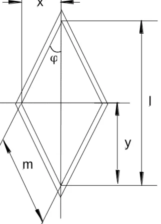
where x, y, b and α are geometric mesh parameters as specified in Fig. 3.1

m

y x

l

φ

Fig. 3.1 Mesh geometry specification.

[image:48.595.175.336.458.681.2]

(49)

35

Baranov (1960) considered the shape of a plane net under uniformly distributed vertical loads (Fig. 3.2). The properties of the net were perceived through the properties of the individual mesh. It was shown that tensions in individual twines depend on the hanging coefficients. The relation of the horizontal tension

σx and the vertical tension σy appeared as follows:



2 2

tan 1

         

y x

x y

u u f f

3.5

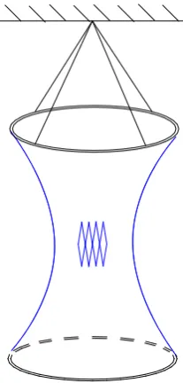
[image:49.595.277.381.388.605.2]

Fridman (1973) stated that if the bottom and top meshes of the net are attached to rings, the net narrows towards the middle due to tensile forces (Fig. 3.3). Hence, based on Baranav’s considerations, it can be assumed that the shape of the net restrained between the hoops depends solely on the hanging coefficients, hoop diameter and a number of meshes between the hoops.

Fig. 3.3 A net sample attached to two hoops.

(50)

36

3.3 Test objective

The current study measured mesh opening in the middle section of hoop units for netting attached in both longitudinal (standard) and transverse (T90) directions. When the longitudinal net orientation was aligned with the vertical axis, the middle section hanging coefficient and distance between the hoops were not affected significantly by a vertically applied load. The extent of variation depended on the material’s elongation properties (tension stiffness) only. When the net was attached to the hoops in T90 configuration such that the low transverse mesh opening was aligned with the vertical axis, the net tended to acquire a cylindrical shape and not an hourglass shape when no load or small load was applied (Fig. 3.4a). As the load increased, the low vertical mesh opening shifted towards the extended opening of the standard case where the mesh-stretch direction was aligned with the axis of the hoop units (Fig. 3.4b, c). The objective of the experiment was to measure vertical mesh opening in conjunction with a load change for the T90 case until it reaches the vertical opening of the standard case.

(b) (c)

[image:50.595.172.486.407.693.2]

(a)

(51)

37

3.4 Experimental set up

A net sheet with an equal number of meshes (39 x 39) in the longitudinal and transverse directions was restrained between two aluminium hoops. The entire system was of an hourglass shape – the top hoop was hung from a single point, and a platform was attached to the bottom hoop for applying weights (Fig. 3.3). The hoop was of 385 mm outside diameter, 22 mm thickness and 700 g weight. Prior to the attachment, the vertical sides of the net sheet were stitched together with a 24ply PE (polyethylene) twine so the sample acquired an enclosed shape. The net was attached to the hoop by twine lacing trough a mesh and around the hoop (Fig 3.5).

Fig. 3.5 The net laced to the hoop.

When the net was attached to the hoops in the longitudinal orientation, a load of 10kg was applied for the net to overcome mechanical forces and to acquire a firm and symmetrical shape. Three threads were connected to the top hoop equally-spaced along the hoop circumference, and lowered vertically with sinking weights (Fig 3.6). As three measurements of k (the distance between the middle section and the thread (Fig. 3.6b) were taken, it ensured that the system was symmetric in respect to the vertical axis. The results for the measured distance k allowed circumference c0 and hanging coefficient u0 calculations for

(52)

38 ) ( 2

0 r k

c    _3.6

c c u

u₀  _x ₀/

3.7

where r is outside hoop radius, k is the location length as specified in Fig. 3.6, ux

is a horizontal hanging coefficient of meshes on a hoop, and c is a hoop circumference.

[image:52.595.137.523.391.675.2]

The distance between the hoops was also recorded. As mentioned above, meshes do not open transversely as wide as longitudinally due to knots being aligned in the longitudinal direction. Thus to compare the distance between the hoops in the longitudinal and transverse directions, a correction factor was applied – the factor was equated to the ratio of transverse and longitudinal mesh size (Table 2.1).

(53)

39

transverse and longitudinal orientation. To overcome this, two light-weight hoops of 100 g each were made from polyethylene pipe to test the Dyneema® sample (Fig. 3.6a).

As the mesh size slightly varied between the samples (and hence hanging coefficients also varied), it was important to check the extent to which the hanging coefficient for meshes attached to the hoops affected the distance between the hoops. For this, another set of experiments were done with nylon samples (50mm mesh size, single-knotted and twisted twine of 1466Rtex, eq. 2.1 defines Rtex). For every sample, a number of meshes between the hoops were constant, but the number of meshes attached on to the hoops varied. The horizontal hanging coefficient was calculated as shown in eq. 3.8:

nl c u_x 

3.8 where c is a hoop circumference, n is a number of meshes attached to the hoop,

and l is mesh size. The number of meshes on the hoop n and the resulting

hanging coefficients ux are presented in Table 3.1.

Table 3.1. A number of meshes attached to the hoop and corresponding hanging coefficient (eq. 3.8) for four nylon samples.

number of meshes on hoop n 183 159 147 135

hanging coefficient ux 0.32 0.37 0.40 0.44

(54)

[image:54.595.223.437.71.352.2]

40

Fig. 3.7 Nylon samples in the longitudinal orientation attached to 1m diameter hoops with the horizontal mesh hanging coefficient of 0.32 and 0.44 (eq. 3.8 and

Table 3.1). As seen, the distance between the hoops does not significantly change with hanging coefficient variation.

As mentioned above, Andreyev (1960) developed a series of elliptical equations that estimate the shape of the net restrained between the hoops in the longitudinal orientation. As a part of the present study, a Matlab code was developed to solve the equations to compare analytical and experimental results for the longitudinal orientation. The code is presented in Appendix I.

3.5 Experimental results and discussion

Hanging coefficient effect on the distance between the hoops

A change in the distance between the hoops in respect to the hanging coefficient ux for nylon netting is presented in Table 3.2. The distance k linearly changed

with respect to the hanging coefficient ux – as the hanging coefficient increased

(55)

41

was only a 3.6% difference between the highest and lowest hanging coefficients (due to slight variation in mesh size). Thus, as a high increase of 35% in the hanging coefficient caused only 2% variation in the distance between the hoops, a 3.6% change in the hanging coefficient was assumed to be negligible.

Table 3.2 Measurements for nylon samples.

hanging coefficient ux 0.32 0.37 0.40 0.44

distance k, mm (Fig 4.6) 67 90 104 127

distance between hoops Lhoop, m 2.39 2.38 2.37 2.36

Experimental results vs. analytical prediction

The distance between the hoops for the longitudinal orientation for the nylon samples (Table 3.2) was compared with the analytical prediction by Andreyev (1960). The difference in results was about 1%. However, the theory proposed by Andreyev (1960) can only predict the distance between the hoops based on the circumference of the middle section c0 (eq. 3.6) which is often unknown.

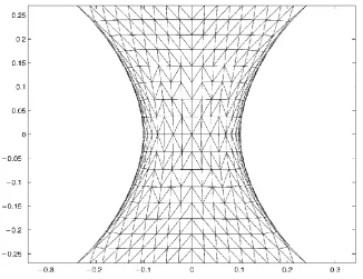
Prior (2001) numerically estimated the shape of a net that was restrained between the hoops (Fig. 3.8). However, as there was no prior knowledge for the netting flexural rigidity figures, the proposed model did not accurately estimate the shape.

Mesh resistance for bending

(56)

42

[image:56.595.169.496.144.395.2]

on y-axis of Fig. 3.10 is the ratio of middle section mesh opening (eq. 3.6 and 3.7) in the longitudinal orientation to mesh opening in the transverse orientation.

Fig. 3.8 An example of calculated net shape using numerical method of Prior (2001).

(57)

[image:57.842.92.755.134.468.2]

43

Fig. 3.9 Transversely-oriented net sample under various loads.

(58)

44

[image:58.595.149.538.388.638.2]

As seen from Fig. 3.10 initial loads bent the twine more effectively - an increment of 0.5 kg caused a significant change in mesh opening for the loads of up to 3kg, while an effect of load increase over 3kg on the mesh opening was less pronounced. The mesh opening coefficient on y-axis of Fig. 3.10 does not reach a figure of 1, which would imply mesh opening in the transverse and longitudinal orientation was equal. The mesh opening for the two orientations could not be equal because the mesh opening in the transverse orientation was restricted by knots being aligned in the longitudinal orientation. If a significantly higher load than in these experiments were applied, it would only cause net damage. The trend lines shown in Fig. 3.10 suggest that the power exponent of the curves approximates to the figure of 0.05. A linear regression analysis was applied to standardise the exponent between the curves. The coefficients a of the power functions y=ax0.05 from Fig. 3.10 can be then used for relative stiffness comparison between the samples.

Fig. 3.10 Mesh resistance to stretch in the transverse direction for three samples (Table 2.1). A mesh opening coefficient (y-axis) is the ratio of mesh opening in

the longitudinal orientation to mesh opening in the transverse orientation.

y = 0.8925x0.0583 _{y = 0.848x}0.0597

y = 0.8207x0.0656

0.70 0.75 0.80 0.85 0.90 0.95 1.00

0 2 4 6 8 10 12

co e ff ici e n t fo r m e sh o p e n ing resist a n ce load, kg Hampidjan

Standard net (24 PE) Euroline

y = 0.913x0.05

y = 0.863x0.05

(59)

45

Table 3.3 A relative stiffness between the samples (Table 2.1)

Sample retail name Trend line coefficient a of the function y=ax0.05

(Fig. 4.10)

A relative stiffness increase

Ultracross Dyneema® _1.0 _benchmark

Hampidjan Dyneex _0.913 _10%

24 ply PE _0.863 _16%

Euroline Premium Plus _0.840 _19%

As no measurable difference was detected for Dyneema®, the coefficient a for this sample was assumed to be 1 in the linear function of y=ax, and the sample was perceived as a low bending stiffness benchmark. Then a relative increase in stiffness for Hampidjan, 24ply PE and Euroline can be said to be 10%, 16% and 19% respectively from the benchmark stiffness.

Flexural rigidity

Eq. 3.1 can be rearranged to give:

2 cos 2 cos 4 cos                   _              m a x f

EI _x _3.9

Similarly, eq. 3.2 can be rewritten to estimate flexural rigidity using mesh opening and tension in y-direction. As seen from eq. 3.3 and 3.4, the horizontal and vertical hanging coefficients (uxand uy respectively) are interchangeable and

can be expressed as follows:

5 . 0 ) 1 ( _y x u

u  

3.10

(60)

46 ) 1 ( ) ( 2 2 5 . 0 2 2 x x x x u u f f f    3.11

A horizontal component of the tension fx then can be expressed as:

5 . 0 4 2 2 ) 1

( _x _x

x x u u fu f    _3.12

Similarly, the vertical component of the tension fy is:

5 . 0 4 2 2 5 . 0 2 2 ) 1 ( ) ( y y y x y u u fu f f f      3.13

Then, splitting the load f into fx and fy components with eq. 3.12 and 3.13, and

(61)

47

Table 3.4 Flexural rigidity figures for 24ply PE (parameters are defined in eq. 3.1).

f fy fx β θ EI

(kg) (kg) (kg) (Nmm2)

1 1.0 0.17 -2.19 0.4 59

1.5 1.5 0.23 8.12 0.4 61

2 2.0 0.29 1.66 0.4 58

2.5 2.5 0.36 1.59 0.4 59

3 3.0 0.43 1.52 0.4 56

5 4.9 0.72 1.42 0.4 56

7 6.9 1.00 1.37 0.4 54

9 8.9 1.29 1.33 0.4 49

11 10.9 1.57 1.32 0.4 52

Fig. 3.11 Flexural rigidity as a function of twine linear density: data from Sals et al. (2007) (blue dots), and present study (red dots).

Sals et al. (2007) obtained flexural rigidity figures for net samples of a wide range of twine linear density - for very stiff nets with linear density between 5 and 20kRtex, a linear relationship between flexural rigidity and twine linear density was suggested. However, in a case of low twine linear density, a linear dependence of flexural rigidity on twine linear density is less pronounced (Fig. 3.11). When the results from the current study are considered together with Sals

0 20 40 60 80 100

0 2 4 6 8

flex

u

ral

ri

g

idity

,

Nm

m

2